Article

Simulative Investigation of Different DLD Microsystem Designs with Increased Reynolds Numbers Using a Two-Way Coupled IBM-CFD/6-DOF Approach

1
Institute for Particle Technology, TU Braunschweig, 38104 Braunschweig, Germany
2
Center of Pharmaceutical Engineering (PVZ), TU Braunschweig, 38106 Braunschweig, Germany
3
Institute for Microtechology, TU Braunschweig, 38124 Braunschweig, Germany
*
Author to whom correspondence should be addressed.
Processes 2022, 10(2), 403; https://doi.org/10.3390/pr10020403
Submission received: 28 January 2022 / Revised: 14 February 2022 / Accepted: 16 February 2022 / Published: 18 February 2022
(This article belongs to the Special Issue Computational Modeling of Multiphase Flow (II))

Abstract

:
Deterministic lateral displacement (DLD) microsystems are suitable for the size fractionation of particle suspensions in the size range of 0.1 to 10 µm. To be able to fractionate real particles beyond a laboratory scale, these systems have to be designed for higher throughputs. High flow resistances and increasing the clogging of the systems impose substantial challenges for industrial operation. Simulative parameter studies are suitable for improving the design of the systems; for example, the position and shape of the posts. A high-resolution, two-way coupled 6-DOF CFD-DEM approach was used to study the flow and particle behavior of different post shapes (circular and triangular) and post sizes at different Reynolds numbers. The results were compared with the classical first streamline width theory. It was shown that the streamline theory does not account for all effects responsible for the separation. Furthermore, a shift in the critical particle diameter to smaller values could be obtained when increasing the Reynolds number and also when using triangular posts with reduced post sizes compared to the post spacing. These findings can help to improve the efficiency of the systems as the post spacing could be extended, thus reducing the flow resistance and the probability of clogging.

1. Introduction

The particle size of pharmaceutical ingredients is of great importance as it affects their dissolution rate, as well as bioavailability, and, in formulations, controls the drug release rate. To obtain safe drugs, formulations with defined particle sizes and narrow size distributions must be produced [1]. One way to control the particle size is via subsequent fractionation using microfluidic devices. Various methods for sorting micron and submicron particles have been described, such as pinched flow fractionation (PFF), multiorifice flow fractionation (MOFF), crossflow filtration, microfluidic centrifugation and deterministic lateral displacement (DLD) [2,3]. Crossflow filtration, a fluidic separation process designed to prevent particle deposition, is not very efficient in the particle size range of approximately 50 to 500 nm because diffusion and hydrodynamics have a minimum effectiveness [4].
The deterministic lateral displacement (DLD) method is a passive microfluidic separation technique that has been successfully used to sort and isolate various biological particles, such as tumor cells and blood components. It is capable of separating particles precisely and with a high resolution based on their size, shape and deformability [5]. DLD microarrays consist of channels interspersed with a large number of regularly arranged post obstacles (Figure 1). These obstacles are disposed in consecutive rows with a lateral shift (δ) in each row perpendicular to the main flow direction. N defines the periodicity of the array, meaning that, after N rows, the posts recurrently reach their initial lateral position. Assuming laminar flow, the arrangement of the posts results in a characteristic flow pattern in which the flow splits into N streamlines between adjacent obstacles. The width of the streamline in direct contact with the post determines the particle’s critical particle diameter (dc). If the radius of the particle is smaller, it will remain within the streamline and will consequently move through the system on a zigzag path. If it is larger, the particle is repeatedly lifted out of the first streamline into the second streamline. This leads to a lateral movement of the particle, which can be described by the angle θ = arctan δ/Rd in relation to the main flow direction, with Rd being the center-to-center distance between each post row [6].
The DLD method has traditionally been operated in a creeping laminar flow—many studies on this can be found in the literature [5,7]. At these low Reynolds numbers, the flow rate is restricted to a µL/min range [8]. Furthermore, since the method is limited to rather dilute particle concentrations, it still requires improvement to increase its sample throughput and particle concentration to an industrially relevant extent [9]. There are several limiting factors encountered in increasing the throughput: the high number of small post structures causes large flow resistances, for which, the microsystem and periphery must be dimensioned. Parallelizing multiple microsystems or using very deep arrays is one way to increase the throughput, but the latter is limited by fabrication technology [5]. Increasing the flow rate is another possibility for increasing the throughput. However, it must be noted that increasing the Reynolds number changes the flow pattern, which affects the separation [10]. There has already been some research on the use of higher flow rates in recent years [8,11,12,13,14,15]. The main findings are that increasing the Reynolds number reduces the dc, and that static vortices form behind the posts starting at a Reynolds number of 15 to 20 [10].
Although the gap size is larger than the particle size in DLD microsystems, in contrast to conventional filtration techniques, the clogging of DLD systems is a major challenge. Clogging changes the flow field around the affected zone and, therefore, affects the separation efficiency. There are several studies on the use of different post shapes to influence the flow in the gap between two posts, which is critical for separation [5]. Triangular post shapes, for example, cause an asymmetry of the velocity profile between the posts, resulting in a narrowing of the first streamline and, thus, the critical particle size. In other words, the gap can be increased to keep the dc constant, reducing the tendency of the system to clog [16].
Various numerical methods have been used so far to characterize the flow and particle behavior in DLD microsystems. A distinction can be made between calculations of the steady-state flow field [14,17,18,19,20,21] and simulations that include particle dynamics [8,15,22,23,24,25,26,27,28,29,30,31,32,33,34]. The calculation of the velocity field only allows for an estimation of the behavior of particles in the flow and the dc, but the interactions between particles and the fluid are neglected. The fluid–structure interactions are either calculated in direct numerical simulations (DNS) [25,26,27,28,29,32] or the fluid and solid phases are calculated in separate processes, and both methods are coupled iteratively; for example, the lattice Boltzmann method (LBM) coupled with the discrete element method (LBM-DEM) [30] or coupled with the finite element method (FEM) [31]. The fluid–structure simulations were either simplified into two dimensions [8,15,22,23,24,28,32,34,35] or calculated in a more complex three-dimensional way [25,26,27,29,30,31]. In addition, the calculations differ in whether only the forces (and moments) that the fluid exerts on the particles are calculated (one-way coupling) [11,23] or whether particle feedback to the fluid takes place (two-way coupling) [22,24,26,27,28,36].
One-way coupled simulations of particle-laden flows reproduce the behavior of the particles in the flow but ignore the fact that the particle in the gap affects the velocity field and thus changes the streamlines. The use of two-dimensional coupled simulations saves computational costs, but it ignores the fact that particles in fluids move in a three-dimensional mode and that deviations are to be expected in the forces on the particles [37]. Some works also consider particle rotation in their calculations, allowing for rotation-induced lift forces [25,26,28,30,33]. Only few works dissolve or model short-range repulsive viscous (lubrication) forces [9,29,32,33]
In this work, a model was developed to represent particle transport within a DLD microsystem. The immersed boundary method (IBM) was used to couple computational fluid dynamics and the discrete element method using a two-way six degrees of freedom (6-DOF) process with lubrication correction. The model is used to run through a variety of parameter combinations. It is intended to mimic the behavior of the particles in the microsystem as realistically as possible. In addition to evaluating the particle trajectories and, thus, assessing the ability of the model to predict fractionation effectiveness, the results of the dc values determined from fluidics using streamline widths will also be evaluated and assessed. The influence of the Reynolds number at different post shapes and sizes will be investigated, with the objective of increasing the throughput of microsystems and improving their performance.

2. Materials and Methods

2.1. Model Description

In our simulation setup, we aim to model a scenario of a DLD microsystem that is as realistic as possible in order to fractionate particles in the range of 1 to 10 µm. Therefore, a three-dimensional fragment of a microsystem was considered, consisting of 10 rows of posts with 10 posts per row. A periodicity of N = 10 was chosen, which corresponds to a lateral row shift of δ = 0.1 µm. The height of the microsystem in the direction of the axis of the posts is 10 µm. A block-structured grid was created around the posts to discretize the flow field according to the finite volume method. The grid resolution was set to a number of 24 cells over the gap length, based on grid studies. Since at least eight cells per particle diameter are necessary to provide accurate results for the coupling, the mesh was additionally dynamically refined by one more level locally in the area around a particle. Inlet and outlet areas, normal to the flow direction, were provided with cyclic boundary conditions for the pressure and velocity. The walls parallel to the flow, as well as the post walls, were given Dirichlet boundary conditions for the velocity—those orthogonal to the post axis with a slip condition, and the lateral walls, as well as the post walls, with a no-slip condition. Neumann boundary conditions were specified for the pressure on these patches. Cyclic boundary conditions were not chosen for the lateral boundaries, since they induced an artificial anisotropy in the velocity field. This means that the velocity averaged over the simulation field in the case of lateral cyclic boundary conditions has a nonzero lateral component, as already observed by [38,39], which affects the periodicity of the system [30]. In contrast, when choosing wall boundary conditions in the lateral direction, a pressure gradient normal to the flow was observed, highlighting that cyclic boundary conditions in this direction are unsuitable.
The particle simulation domain was also equipped with cyclic boundary conditions in the inlet and outlet, which means that the particle passes through several periods within the domain. The post walls, as well as the walls aligned parallel to the flow, were defined as frictional walls. The fluid flow is driven by a force that controls a predetermined constant velocity averaged over the inlet patch. In this way, Reynolds numbers 1, 10, 30 and 50 were set (calculated as in [10]). With a constant post gap of approximately G = 10 µm (with slight deviations due to edge rounding induced by the meshing), simulations were performed with post heights of H = 10 µm and H = 5 µm. The row distance is Rd = 20 µm for a post height of H = 10 µm and Rd = 15 µm for H = 5 µm. In addition, the post shape was varied, i.e., simulations were performed with cylindrical posts and equilateral triangular posts. Individual simulations from one particle, each with successive diameters of 2, 3, 4 and 5 µm, were performed for all parameter combinations of post shape, size and Reynolds number. An overview of the simulation parameters can be found in Table 1. One single particle was induced near the inlet between the third and fourth lateral post and lasted for approximately four periods.
The time derivatives were discretized by the Euler method. The divergence, gradient and Laplacian terms were discretized by the Gauss linear method.

2.2. Equations

The particle-laden flow was modeled using a coupled CFD-DEM approach [40]. In this method, the fluid phase and solid phase are first calculated separately. In the fluid phase, the presence of the particles is initially not taken into account [41]: to obtain the pressure and velocity fields, the continuity equation and the momentum conservation equation are solved. The continuity equation states that the mass in a volume element moving through the system is constant:
ρ t + · ( ρ u ) = 0 .
The momentum conservation equation describes the change in momentum of a fluid element over time, which can be divided into a local and a convective part on the left side and consists of a pressure term, a deviatoric stress term and an external force term on the right side:
ρ D u D t = ρ ( u t + u · u ) = p + · τ + ρ f .
Assuming a Newtonian fluid, the deviatoric stress term τ consists of the strain rate tensor minus the divergence of the velocity field. Since the Mach number is below the critical value for compressible flows (Ma = 0.3), the flow can be assumed to be incompressible. Assuming a constant density, the equations can by divided by it, and the divergence of the velocity field is zero. The continuity equation simplifies to:
· u = 0
and the momentum equation becomes the Navier–Stokes equation for incompressible fluids:
D u D t = u t + ( u · ) u = 1 ρ p + υ Δ u + f .
OpenFOAM solves the so-called Reynolds-averaged Navier–Stokes (RANS) equations. Here, turbulent effects are represented by a time variation around an averaged flow and are modeled as an additional viscosity. Since we do not yet have such randomly varying components in the covered regime and, despite vortex formation, the fluid elements move in ordered paths, the flow can still be described as laminar and the turbulence term could be eliminated [42]. The method used here to solve the Navier–Stokes equations for incompressible flows is called PISO (pressure-implicit with splitting of operators) [43]. The generalized geometric algebraic multigrid (GAMG) solver was used to solve the pressure equation, and the smooth solver was used to solve the velocity equations.
In terms of particle simulation, the following differential equations (Newton–Euler) for translational and angular momentum were calculated:
m u t = F g + F f + F p p w
I ω t = a × ( F f + F p p w ) ,
where m is the mass of the particle, I is the second moment of area, ω is the angular velocity, a denotes the center-to-surface vector and Fppw represents the particle–particle or particle–wall collision forces. Via Ff, an additional drag force is introduced, which the fluid exerts on the particle. Fg describes the gravitational body force on the particle [44].
The coupling between particle simulation and fluid dynamics is realized by the immersed boundary method (IBM), introduced by Peskin [45]. In this method, the flow around arbitrarily shaped bodies can be calculated. For this purpose, the flow field is solved on a fixed Eulerian grid and the immersed boundary is represented with a Lagrangian grid. This is useful for the analysis of flows over complex time-varying surfaces where spatial discretization is challenging. The need to remesh the flow field around the body at each time step would require an enormous computational effort. Additionally, for particle-laden flows, the interface between different phases must be accurately tracked and resolved [46]. Thus, Hager developed a solver in which the discrete element method (DEM) software LIGGGHTS is coupled with the computational fluid dynamics (CFD) software OpenFOAM via the IBM [47]. The algorithm operates as follows: first, the initial and boundary conditions of the CFD are read and the initial positions and velocities of the particles are transmitted. Then, for all cells that overlap with a particle, the void fraction is determined. Velocity and pressure fields are corrected accordingly, and fluid forces, as well as torques, are calculated and transmitted to the DEM. This is followed by a phase in which, as described, the Navier–Stokes equations are solved independently on the CFD side and the Newton–Euler equations on the DEM side. In the next coupling step, the new particle positions and velocities, which have changed due to collisions and fluid forces, are transmitted to the CFD. The CFD corrects the velocity, as well as pressure, in the cells that intersect with particles, and transmits new fluid forces, as well as torques, to the DEM, again solving the independent differential equations. This process is repeated until the end of the defined simulation time [44].

2.3. Force and Moment Calculation

The components of the forces and moments included in Equations (5) and (6) will be described in more detail in this section. For the derivation of the drag force, Ff, the stress, t Γ s , between the fluid and a solid surface, Γs (such as particles and post walls), has to be considered, which can be described as the product of the fluid stress tensor σ and the surface vector n ^ , accordingly:
t Γ s = σ · n ^ ,
t Γ s can be transformed into the drag force by integration over Γs. To prepare it for the finite volume method the surface integral can be converted into a volume integral over the solid volume, Ωs, by applying the divergence theorem, hence:
F f = Γ s σ · n ^ d Γ s = Ω s · σ d Ω s ,
which leads to the following expression for an incompressible Newtonian fluid, indicating that the force consists of a pressure term and a viscous term:
F f = Ω s p + υ ρ 2 u d Ω s
To calculate the fluid torques, the viscous part of the force term is used to calculate the cross product with the position vector, corresponding to:
M f = Ω s a × υ ρ 2 u d Ω s .
In the software, the volume integrals of fluid forces and torques are calculated in a discrete form, applied to the cells intersecting with solids and integrated numerically [44].
The effect of gravitational body force (Fg) and buoyancy force (Fb) is negligible in these simulations, since we chose the same density for the solid phase as for the fluid phase.
For the derivation of the collision forces, Fppw, it is important to consider that the hydrodynamic interactions between particles and a post wall may not be fully represented. Short-range interactions may be underrepresented, since this would require a strong local refinement of the mesh, which would greatly inflate computation times due to the small cell size [48]. To compensate for this, a lubrication correction model was implemented for small solid–solid distances. The interplay between the IBM, lubrication correction and contact model is illustrated in Figure 2.
When two solids approach, the lubrication force is completely resolved by the IBM as long as a certain threshold (here referred to as ɛx) is not exceeded. Otherwise a lubrication correction force, Flub (specified by Lambert et al. as tabulated lubrication correction, CLM, Equation (11)), is added [50]:
Δ F i , l u b 6 π η r p u i , p = {   λ ( ε Δ x ) λ ( ε ) , λ ( ε Δ x ) λ ( ε σ ) , 0 ,         ε σ ε < ε Δ x ,     0 ε < ε σ ,     o t h e r w i s e .
The amplification factor (λ) is a function depending on the nondimensionalized distance ɛ = distance/rp, which relies on the properties of the two approaching solids. Instead of choosing the λ for the lubrication interaction between a sphere and a flat wall, we follow the approach of Kulrattanarak et al. [29], who refer to studies by Adamczyk et al. [51] on the approximation between a sphere and a cylinder. Accordingly, the lubrication force between a sphere and a cylinder is similar to the force between a sphere and a second sphere whose radius is twice the radius of the cylinder [29,51]. To approximate this force, Jeffrey’s equation for approximating unequal spheres with equal velocity was used as the λ [52]. The possible deviation due to the fact that only one of our objects was moving was tolerated. If ɛ falls below a second, smaller threshold, ɛσ, the lubrication correction forces are kept constant. This parameter, ɛσ, is to prevent forces from increasing infinitely when two solids come very close to each other, which could cause instabilities. ɛσ can also be considered as surface roughness [49,50,53,54]. In this work, analogous to [29], a value of ε σ = 0.05 was chosen, which is in the order of magnitude of the post wall roughness we observed in the manufacturing process.
In order to validate Flub, a single particle was moved slowly frontally toward a single post and the dimensionless force was plotted against ɛ, comparing the uncorrected IBM to Jeffrey’s analytical solution and to the corrected IBM (Figure 3). It should be noted that the CFD mesh cell size in the simulation case is not made dependent on the particle size, and thus the larger particles are represented by a larger number of cells. Therefore, the smaller particles may require more assistance from the lubrication correction model than the larger particles. The test simulations show that, for the smaller particle sizes, velocity deviations between the analytical solution and the uncorrected IBM arise at a larger distance between particles and a post wall. Therefore, a larger threshold, ɛx, has to be chosen for the smaller particles than for the larger ones (see chosen values in Figure 3). The test simulations also show that the corrected IBM matches the analytical solution sufficiently well.
It was observed that omitting the lubrication correction resulted in a strong torquing of the particles upon wall contact and that the particle paths were significantly affected as a result of their rotation. This might represent the behavior at high wall roughness, where the particles are less decelerated at wall contact.
Once the two solids are in direct contact, the DEM contact model will become active. Here, the contact model according to Hertz and Mindlin is applied, which describes the normal and tangential forces acting on a particle at the contact points [55,56]. The normal force, FN, is calculated according to Equation (12). Here, EM is the mean modulus of elasticity, rP,M is the mean particle radius and δN is the overlap of the touching solids in normal direction to the contact surface:
F N = 4 3 E M r P , M δ N 32 .
In addition, the damping force FN,D, with the coefficient of restitution e, the mean particle mass mP,M and the relative velocity of the contact point in the normal direction vN,rel, acts according to the following equation:
F N , D = 2 5 6 ln e ln 2 e + π 2 2 E M , i j r P , M δ N m P , M υ N , r e l .
For the force tangential to the contact surface FT with the Poisson ratio ν:
F T = 8 E 2 + 2 υ r P , M δ N δ T .
Here, likewise, a damping force, FT,D, operates tangentially to the contact surface:
F T , D = 2 5 6 ln e ln 2 e + π 2 8 G M , i j r P , M δ N m M υ T , r e l .
Furthermore, the static friction force, FC, between the two contacting solids is taken into account, which includes the static friction coefficient µ [57]:
F C = μ F N .
A summary of the simulation parameters can be found in Table 2.

3. Results and Discussion

In the following, the critical particle diameters (dc) will be presented and compared. The dc values were determined in two different ways: first, by determining the width of the first streamline (we refer to it as the fluidic dc), and, second, by evaluating the particle trajectories. In this way, whether the determination of the dc via the streamline width is representative for the actual separation will be analyzed, which could avoid more complex coupled simulations in the future.
The various variables influencing the dc, i.e., post shape, size and Reynolds number, will be investigated. The feasibility of the simulation setup will be validated by comparing it with the current literature.

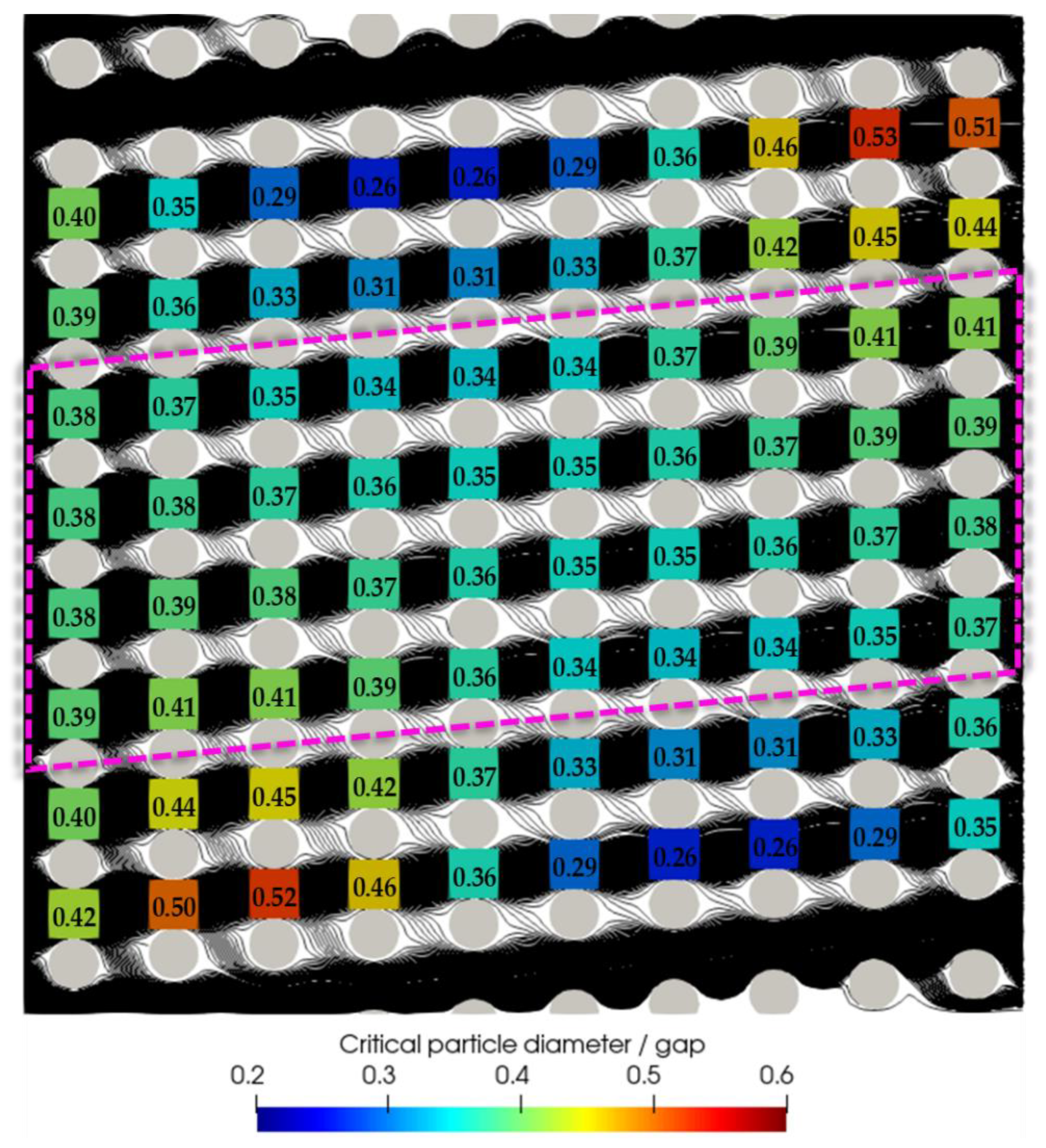
3.1. Calculation of Fluidic dc Distributions

To avoid the issue where periodic boundary conditions in the direction of the post offset lead to artificially induced permeability normal to the main flow direction, walls were used instead. However, Pariset et al. have shown that, for a small number of posts across the main flow direction, wall effects lead to different dc values within one system [58]. The reason for this is mainly due to the design of the posts at the wall: in the sections where posts merge with the wall, the streamlines are pushed away from the wall. In the sections where no posts intersect with the wall, the streamlines are pushed to the wall. This leads to a shift in fluidic periodicity, which affects the dc. This effect is still visible further away from the walls [58]. To keep this effect on the particle trajectories low, the particles were introduced into the system between the third and fourth posts in the lateral direction. To obtain an idea of how large the variance in streamline widths is within our simulation case, we inspected them in more detail: Figure 4 shows the streamlines and the estimated distribution of dc at Re = 1 and H/G = 1. The dc values were determined by estimating the first streamline widths using the local velocity profiles in the gaps between adjacent posts and the local fluidic periodicities using the equation by Reinecke et al. [30]. This was performed by dividing the area under the velocity profile by the local fluidic periodicity, so that each section acquired the same fractional area. Our results show that if the area up to the third post from the lower and upper wall is disregarded (highlighted in Figure 4), the dc as a proportion of the gap ranges between 0.34 and 0.41. We accept this deviation for the significance of our results. In order to obtain a higher accuracy, the number of posts in the lateral direction would have to be increased significantly, at the expense of the computing capacity. In the real case, the periodic recurrence of the effect should cause the unwanted shift of the particle path to compensate, to some extent, for the chip length.

3.2. Parameter Variation in Fluidic dc

In the following, the results of the first streamline width as a function of the different parameters will be compared. Figure 5 shows the mean dc values with standard deviations, determined from the first streamline widths. They are differentiated by the post shape, as well as the H/G ratio, and plotted against the Reynolds number. Qualitatively, the largest dc values are found for larger H/G ratios and cylindrical posts. Small H/G ratios and triangular posts lead to an overall decrease in dc. Explanations are provided by Figure 6. At Re = 1, slightly more plug-like velocity profiles between neighboring posts occur at smaller H/G ratios for cylindrical posts, and a slight asymmetry occurs for triangular posts. Both result in dc values being reduced to a similar degree. Increasing the Reynolds number leads—for all post shapes and size ratios—to an asymmetry of the flow profile towards the lower post, as Dincau et al. have already indicated [8]. This causes the largest overall reduction in dc. However, the reduction in dc for the triangular posts compared to the cylindrical ones with H/G = 1 becomes smaller as the Reynolds number increases. Interestingly, the velocity profile for cylindrical posts and H/G = 0.5 shows the strongest overall asymmetry and corresponding lowest dc.
Looking at the standard deviation, it is noticeable that an increased Reynolds number leads to a larger variance in the dc values. Additionally, a larger H/G ratio leads to wider dc distributions. The narrowest distribution is seen at H/G = 0.5 and round posts. This is to be expected, since proportionally smaller obstacles have less influence on the flow field. Triangular posts lead to somewhat wider distributions, presumably due to sharper deflections of the streamlines and an increased vortex formation.

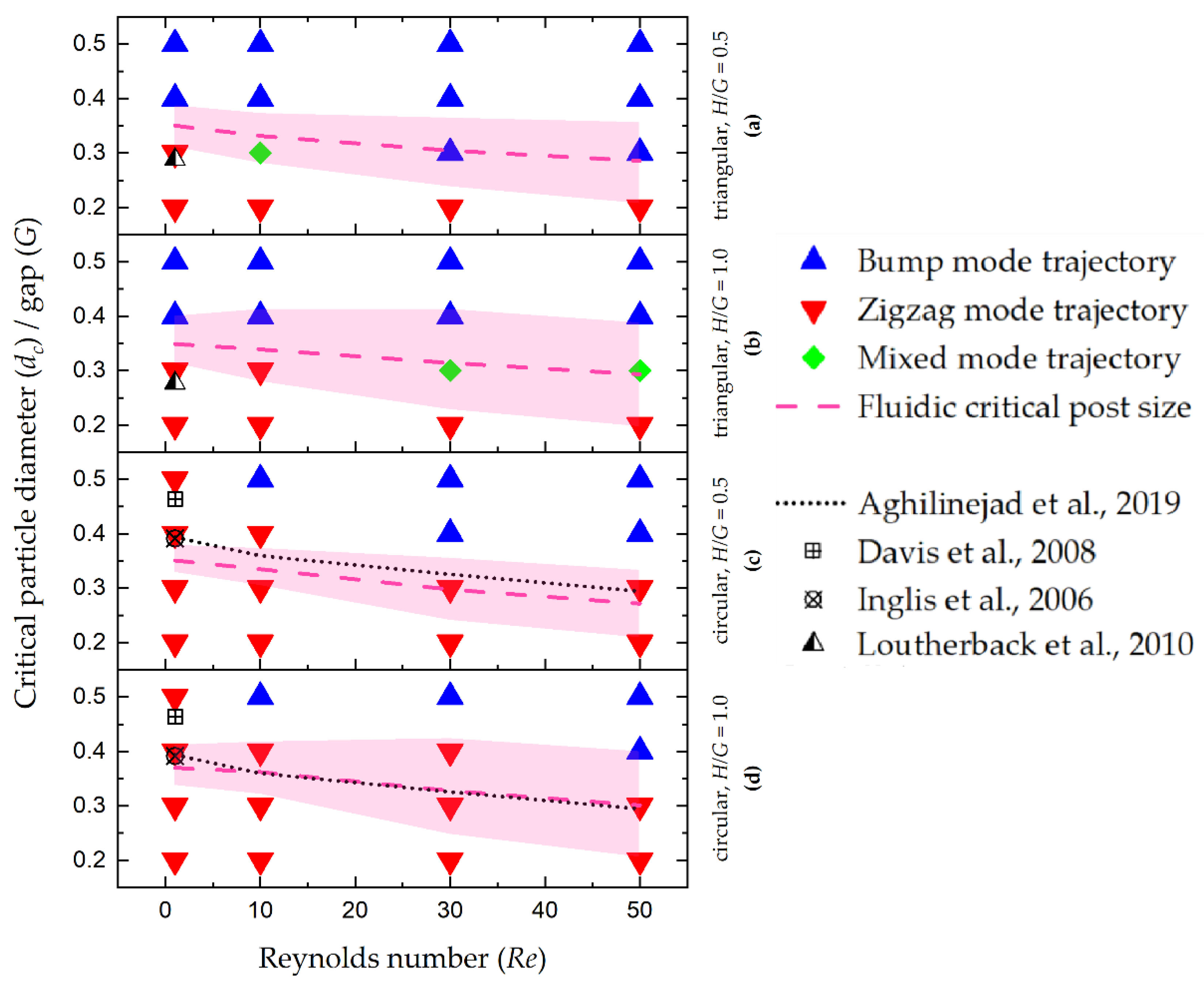
3.3. Particle Trajectory dc and Validation of Results

In the following, the simulated dc values will be compared with the literature in order to obtain an impression of the significance of the results; subsequently, the results from the CFD (fluidic dc) are analyzed against the results of the coupled CFD-DEM simulations (particle trajectories).
The results of the dc as a proportion of the gap over the Reynolds number are shown in Figure 7. for both the streamline-based calculated dc values and the particle trajectories. The results are divided into cylindrical posts with a circular base (c and d) and posts with an equilateral triangular base (a and b). A distinction is also made between post-height-to-gap ratios, H/G, of 1 (b and d) and 0.5 (a and c). The mean fluidic dc values calculated based on the first streamline widths are shown as dashed purple lines. Shown in light purple around the dashed lines are the dc ranges up to the minima and maxima within the zone in which the particle traverses (marked area in Figure 4). The particle trajectories are color-coded according to whether they follow the bump, zigzag or mixed mode (also called altered zigzag, i.e., a path that is between bump mode and zigzag mode). The particle trajectories marked as mixed-mode are probably due to the locally different dc values, since, in both cases, the particle path changes from the bump to zigzag mode by the time the trajectory becomes closer to the wall.
To obtain a better overview of existing models for determining the dc for fractionation, the results of calculations from the literature are plotted as well. For cylindrical posts at lower Reynolds numbers, the models of Inglis et al. [59] and Davis [60] were used. Furthermore, the equation of Loutherback et al. [16] was used for a comparison with triangular posts. Since we are also dealing with Re >> 1, the equation of Aghilinejad et al. [11] was plotted for higher Reynolds numbers.
For Re = 1 the mean fluidic dc is slightly below the value determined by Inglis et al. [59]. Inglis’ equation is based on the assumption that the flow profile between two posts is equal to a parabola and calculates the width of the first streamline by dividing the parabola into N sections with equal area. When the flow passes through two cylindrical posts, the flow profile becomes more plug-like compared to the profile between two straight walls, resulting in a smaller dc. This effect is increased by a smaller H/G ratio as the channel effect is further reduced [7].
Aghilinejad et al. performed simulations with COMSOL Multiphysics® at numerous combinations of offsets and Reynolds numbers, and, by evaluating the particle paths, developed an equation for determining the dc at higher Reynolds numbers [11]. The equation mostly agrees with our dc values determined from the streamline widths for cylindrical posts at a ratio of H/G = 1. This agreement could be explained by the fact that, in the calculation method used by Aghilinejad et al., the particles do not displace the fluid, so the particles do not affect the streamlines. The results of the equation slightly overestimate the results at a ratio of H/G = 0.5. It can be assumed that the underlying simulations were performed at H/G = 1 and that the discrepancy is due to a slightly more plug-like velocity profile between adjacent posts at H/G = 0.5 that is not taken into account by the equation of Aghilinejad.
For the triangular posts, Loutherback et al. [16] have determined the dc by evaluating the streamline widths at different base-to-height ratios of the triangles and different H/G ratios. In the same manner as us, they also used a periodicity of 10. At smaller H/G values, according to Loutherback et al., the velocity profile is more plug-like and less skewed toward the top of the lower post, resulting in a slightly larger dc [16]. This very subtle difference is also noticeable in our results. However, we obtain a higher dc overall, which is due to the slightly rounded vertices caused by the meshing, which, according to Loutherback, reduce the asymmetry effect of the velocity profile [16].
The dc values determined from the streamline widths are only partially reflected in the particle trajectories. In the case of the circular posts, the streamlines predict dc values that are too small. Furthermore, according to particle trajectories, triangular posts can be used to achieve a significant reduction in dc compared to round posts, which is not evident from the streamline width determination. This could be explained by the fact that one of the flow patterns is more stable in relation to the influence of particles. With higher Reynolds numbers, the difference could also be explained by the stronger vortex formation in triangular posts.
Figure 8 shows the velocity vectors for the various post geometries and Reynolds numbers. It can be seen that the flow pattern is not noticeably different for Re = 1 and Re = 10 with circular posts. With triangular posts and H/G = 1, in contrast, a small vortex has already developed. When the Reynolds number increases to Re = 30, a clear vortex can be seen for all post types, which further increases in size at Re = 50. With triangular posts and H/G = 1, the vortex occupies the entire area of the flow wake up to the next post. It can also be seen that the stagnation point in front of the post, where the vectors split into two directions, remains almost at the same height for the circular posts. In triangular posts, on the contrary, the stagnation point moves from the lower to the upper edge as the Reynolds number increases. A change in the position of the stagnation point when vortices occur was already observed by Lubbersen et al. [14] when comparing cylindrical and quadrilateral-shaped posts. Their explanation for why the dc is reduced is that the vortices narrow the gap between two consecutive post rows in the direction of the flow [14]. For rhombic arrays with a gap in the flow direction smaller than the lateral gap, it was found that the dc is proportional to the distance between two successive post rows [7]. The gap between two successive rows of posts is narrowed significantly by the large vortices at high Reynolds numbers. Therefore, it is possible that the presence of vortices at larger Reynolds numbers artificially increases the post size. However, this still does not explain why similar or even smaller dc are measured at lower H/G ratios, since smaller vortices are produced by them.
In addition, Lubbersen et al. expect inertial flow effects and inertial lift forces on the particle to influence the particle behavior [14]. For our results, the differences in the flow wake could also be an explanation for why the dc is lower for triangular posts despite similar results according to the streamline theory. At a higher Reynolds number, the larger vortex possibly causes the particle to rotate. Thus, due to the shear gradient of the vortex, it experiences a lift force that causes it to cross the streamline. Figure 9 shows the paths of the first flow lanes passing below the subsequent posts for both cylindrical and triangular posts at Re = 50 (H/G = 1). As expected, the flow lane for cylindrical posts has the smallest width in the gap and then widens again. For the triangular posts, on the other hand, it hardly increases in width in the flow wake. This could indicate that the particle’s change in the streamline could take place in the flow wake following the gap, driven by the vortex. This would mean that, for triangular posts at higher Re, the location of the streamline crossing is shifted to the flow wake; thus, considering the streamline width in the gap reflects only part of the truth.
Therefore, it can be assumed that there are further factors influencing the separation that are not represented by the simple examination of the streamline width at the narrowest point between two neighboring posts. This hypothesis is supported by the fact that, in the literature, even in creeping flow, the experimentally determined dc was always larger than twice the first streamline [37]. Accordingly, Davis’ empirically determined equation for the dc predicts larger values than the geometrically or simulatively determined equations [60]. Another point is that the theory of the width of the first streamline as a reliable separation parameter assumes that the streamlines remain stable and cannot be influenced by the presence of particles.
In summary, it may not only be the post as a geometrical obstacle that is responsible for a change in the particles between the streamlines. As soon as additional forces act on the particles, such as diffusion, external forces including gravity or an electric/magnetic field, particle inertia or shear-induced forces such as Saffman force and, in the case of rotating particles, Magnus force, deviations from the ideal theory are to be expected. In coupled simulations, these effects can be modeled or neglected. If they are modeled, the required parameters have to be calibrated in an appropriate way to suitably represent the real case.

4. Conclusions

In this work, resolved two-way coupled 6-DOF CFD-DEM simulations were used to analyze the behavior of particles in a DLD microsystem as multiple parameters were varied. A lubrication correction model was added to the simulation environment to adequately represent the viscous forces when particles and a wall approach each other, since the mesh on the CFD side would have to be resolved to a much greater extent for this purpose. For the first time, particle trajectories in DLD arrays with triangular posts were calculated in three dimensions at increased Reynolds numbers considering these different interactions.
With the help of these simulations, it could be shown that the calculation of the critical particle diameter, dc, from pure CFD simulations via the determination of the streamline widths does not represent all effects that matter in the separation in such a system. Considering only the streamline width does not take into account that the particle itself could affect the flow (especially if it comes into contact with the post). This can lead to a failure of the model, especially for technical particle suspensions, where higher solid concentrations are employed for the fractionation. In addition, effects such as particle rotation and particle inertia are not taken into account. However, in the industrial use of DLD fractionation, higher throughputs and, thus, higher Reynolds numbers are required, so these effects cannot be neglected. Furthermore, the streamline model considers the streamline width at the narrowest point between two adjacent posts. Large vortices in the post flow wake could shift this constriction, since the vortex itself acts in a similar manner to an obstacle on the particle, and the streamline crossing takes place at a different location than expected.
Moreover, we were able to show that higher Reynolds numbers have caused a decrease in the dc, applying for all tested post shapes and post size ratios. Following our coupled simulations, the dc values can be further reduced by using triangular posts. Previous concerns were that the flow separation at the sharp edges of triangular posts could avoid the wanted particle fractionation by disturbing the flow pattern at higher Reynolds numbers. Therefore, the risk of clogging can be reduced by widening the distance of the posts. Simultaneously reducing the post-diameter-to-gap ratio provides two benefits: it leads to a further reduction in the dc and wall effects. A widening of the gap in combination with a smaller dc-to-gap ratio reduces the flow resistance and thus relieves the pump systems and periphery. This allows for higher throughputs. In contrast to minimizing the dc by increasing the periodicity, our systems can be shortened, reducing the needed pressure. This represents a step forward in terms of the industrial use of DLD microsystems to fractionate substances, such as pharmaceutical drugs, that are too widely distributed in size or contaminated after particle synthesis and comminution processes.
Nevertheless, it must be noted that, the more elaborate the simulation model is, the more adjustments that are required and the more uncertainties that prevail as a result. Therefore, input parameters, such as friction coefficients and the coefficient of restitution, should be calibrated on the basis of real systems. Another possibility for uncertainties is the lubrication correction model. Many different parameters are involved here. For the viscous forces between a sphere and a rod with a triangular base, there have been no existing studies until now, which is why the values for the approach between a sphere and a cylindrical rod were adopted. The roughness parameter also significantly controls how much the particle is decelerated during contact and to what extent the contact model wins influence. Small changes in the parameters of the lubrication model have caused a high variability in particle behavior. In order to improve the calibration of the model, experimental studies of the deceleration during the approach between particles and posts of different shapes with variations in the wall roughness should be performed. It would also be interesting to color label particles and to study their rotational behavior within the microsystem in order to find out whether the Magnus force has an influence on fractionation. For further development, experiments are planned to confirm the results of the simulations. In particular, the fractionation of different particle concentrations and technical particle suspensions must be investigated.

Author Contributions

Conceptualization: A.K., A.D. and I.K.; methodology: M.S.W.; software: M.S.W.; validation, M.S.W.; formal analysis: M.S.W.; investigation: M.S.W. and J.K.; resources: A.K. and A.D.; data curation: M.S.W.; writing—original draft preparation: M.S.W.; writing—review and editing: I.K., J.K., A.D. and A.K.; visualization: M.S.W.; supervision: I.K., A.K. and A.D.; project administration: A.K. and A.D.; funding acquisition, A.K. and A.D. All authors have read and agreed to the published version of the manuscript.

Funding

This research was funded by Deutsche Forschungsgemeinschaft (DFG) SPP 2045 “MehrDimPart”.

Institutional Review Board Statement

Not applicable.

Informed Consent Statement

Not applicable.

Data Availability Statement

The data that support the findings of this study are available on request from the corresponding author.

Acknowledgments

We acknowledge support by the Open Access Publication Funds of Technische Universität Braunschweig.

Conflicts of Interest

The authors declare no conflict of interest. The funders had no role in the design of the study; in the collection, analyses or interpretation of data; in the writing of the manuscript; or in the decision to publish the results.

References

  1. Shekunov, B.Y.; Chattopadhyay, P.; Tong, H.H.Y.; Chow, A.H.L. Particle size analysis in pharmaceutics: Principles, methods and applications. Pharm. Res. 2007, 24, 203–227. [Google Scholar] [CrossRef] [PubMed]
  2. Sajeesh, P.; Sen, A.K. Particle separation and sorting in microfluidic devices: A review. Microfluid. Nanofluid. 2014, 17, 1–52. [Google Scholar] [CrossRef]
  3. Al-Faqheri, W.; Thio, T.H.G.; Qasaimeh, M.A.; Dietzel, A.; Madou, M.; Al-Halhouli, A. Particle/cell separation on microfluidic platforms based on centrifugation effect: A review. Microfluid. Nanofluid. 2017, 21, 1–23. [Google Scholar] [CrossRef]
  4. Schubert, H. Handbuch der Mechanischen Verfahrenstechnik; John Wiley & Sons: Hoboken, NJ, USA, 2012; ISBN 9783527660704. [Google Scholar]
  5. Salafi, T.; Zhang, Y.; Zhang, Y. A Review on Deterministic Lateral Displacement for Particle Separation and Detection. Nano-Micro Lett. 2019, 11, 1–33. [Google Scholar] [CrossRef] [Green Version]
  6. Dietzel, A. Microsystems for Pharmatechnology: Manipulation of Fluids, Particles, Droplets, and Cells, 1st ed.; Springer International Publishing: Cham, Switzerland; Heidelberg, Germany; New York, NY, USA, 2016; ISBN 9783319269207. [Google Scholar]
  7. McGrath, J.; Jimenez, M.; Bridle, H. Deterministic lateral displacement for particle separation: A review. Lab Chip 2014, 14, 4139–4158. [Google Scholar] [CrossRef] [Green Version]
  8. Dincau, B.M.; Aghilinejad, A.; Hammersley, T.; Chen, X.; Kim, J.-H. Deterministic lateral displacement (DLD) in the high Reynolds number regime: High-throughput and dynamic separation characteristics. Microfluid. Nanofluid. 2018, 22, 1–8. [Google Scholar] [CrossRef]
  9. Vernekar, R.; Krüger, T. Breakdown of deterministic lateral displacement efficiency for non-dilute suspensions: A numerical study. Med. Eng. Phys. 2015, 37, 845–854. [Google Scholar] [CrossRef] [Green Version]
  10. Kottmeier, J.; Wullenweber, M.; Blahout, S.; Hussong, J.; Kampen, I.; Kwade, A.; Dietzel, A. Accelerated Particle Separation in a DLD Device at Re 1 Investigated by Means of µPIV. Micromachines 2019, 10, 768. [Google Scholar] [CrossRef] [Green Version]
  11. Aghilinejad, A.; Aghaamoo, M.; Chen, X. On the transport of particles/cells in high-throughput deterministic lateral displacement devices: Implications for circulating tumor cell separation. Biomicrofluidics 2019, 13, 34112. [Google Scholar] [CrossRef]
  12. Lubbersen, Y.S.; Schutyser, M.; Boom, R.M. Suspension separation with deterministic ratchets at moderate Reynolds numbers. Chem. Eng. Sci. 2012, 73, 314–320. [Google Scholar] [CrossRef]
  13. Lubbersen, Y.S.; Boom, R.M.; Schutyser, M. High throughput particle separation with a mirrored deterministic ratchet design. Chem. Eng. Processing Process Intensif. 2014, 77, 42–49. [Google Scholar] [CrossRef]
  14. Lubbersen, Y.S.; Dijkshoorn, J.P.; Schutyser, M.; Boom, R.M. Visualization of inertial flow in deterministic ratchets. Sep. Purif. Technol. 2013, 109, 33–39. [Google Scholar] [CrossRef]
  15. Dincau, B.M.; Aghilinejad, A.; Chen, X.; Moon, S.Y.; Kim, J.-H. Vortex-free high-Reynolds deterministic lateral displacement (DLD) via airfoil pillars. Microfluid. Nanofluid. 2018, 22, 869. [Google Scholar] [CrossRef]
  16. Loutherback, K.; Chou, K.S.; Newman, J.; Puchalla, J.; Austin, R.H.; Sturm, J.C. Improved performance of deterministic lateral displacement arrays with triangular posts. Microfluid. Nanofluid. 2010, 9, 1143–1149. [Google Scholar] [CrossRef]
  17. Dijkshoorn, J.P.; Schutyser, M.A.I.; Sebris, M.; Boom, R.M.; Wagterveld, R.M. Reducing the critical particle diameter in (highly) asymmetric sieve-based lateral displacement devices. Sci. Rep. 2017, 7, 14162. [Google Scholar] [CrossRef] [Green Version]
  18. Feng, H.; Miskovic, S. Numerical Simulation of Fluid Flow in Deterministic Lateral Displacement Devices. In Volume 2, Fora: Cavitation and Multiphase Flow; Fluid Measurements and Instrumentation; Microfluidics; Multiphase Flows: Work in Progress, Proceedings of the ASME 2013 Fluids Engineering Division Summer Meeting, Incline Village, NV, USA, 7–11 July 2013; American Society of Mechanical Engineers: New York, NY, USA, 2013; p. 07072013. ISBN 978-0-7918-5558-4. [Google Scholar]
  19. Li, Y.; Zhang, H.; Li, Y.; Li, X.; Wu, J.; Qian, S.; Li, F. Dynamic control of particle separation in deterministic lateral displacement separator with viscoelastic fluids. Sci. Rep. 2018, 8, 3618. [Google Scholar] [CrossRef]
  20. Liu, Z.; Huang, F.; Du, J.; Shu, W.; Feng, H.; Xu, X.; Chen, Y. Rapid isolation of cancer cells using microfluidic deterministic lateral displacement structure. Biomicrofluidics 2013, 7, 11801. [Google Scholar] [CrossRef]
  21. Kulrattanarak, T.; van der Sman, R.G.M.; Lubbersen, Y.S.; Schroën, C.G.P.H.; Pham, H.T.M.; Sarro, P.M.; Boom, R.M. Mixed motion in deterministic ratchets due to anisotropic permeability. J. Colloid Interface Sci. 2011, 354, 7–14. [Google Scholar] [CrossRef]
  22. Jiao, Y.; He, Y.; Jiao, F. Two-dimensional Simulation of Motion of Red Blood Cells with Deterministic Lateral Displacement Devices. Micromachines 2019, 10, 393. [Google Scholar] [CrossRef] [Green Version]
  23. Al-Fandi, M.; Al-Rousan, M.; Jaradat, M.A.; Al-Ebbini, L. New design for the separation of microorganisms using microfluidic deterministic lateral displacement. Robot. Comput. Integr. Manuf. 2011, 27, 237–244. [Google Scholar] [CrossRef]
  24. Khodaee, F.; Movahed, S.; Fatouraee, N.; Daneshmand, F. Numerical Simulation of Separation of Circulating Tumor Cells from Blood Stream in Deterministic Lateral Displacement (DLD) Microfluidic Channel. J. Mech. 2016, 32, 463–471. [Google Scholar] [CrossRef] [Green Version]
  25. D’Avino, G. Non-Newtonian deterministic lateral displacement separator: Theory and simulations. Rheol. Acta 2013, 52, 221–236. [Google Scholar] [CrossRef]
  26. Chien, W.; Zhang, Z.; Gompper, G.; Fedosov, D.A. Deformation and dynamics of erythrocytes govern their traversal through microfluidic devices with a deterministic lateral displacement architecture. Biomicrofluidics 2019, 13, 44106. [Google Scholar] [CrossRef] [Green Version]
  27. Henry, E.; Holm, S.H.; Zhang, Z.; Beech, J.P.; Tegenfeldt, J.O.; Fedosov, D.A.; Gompper, G. Sorting cells by their dynamical properties. Sci. Rep. 2016, 6, 34375. [Google Scholar] [CrossRef] [PubMed] [Green Version]
  28. Zhang, Z.; Henry, E.; Gompper, G.; Fedosov, D.A. Behavior of rigid and deformable particles in deterministic lateral displacement devices with different post shapes. J. Chem. Phys. 2015, 143, 243145. [Google Scholar] [CrossRef] [PubMed] [Green Version]
  29. Kulrattanarak, T.; van der Sman, R.G.M.; Schroën, C.G.P.H.; Boom, R.M. Analysis of mixed motion in deterministic ratchets via experiment and particle simulation. Microfluid. Nanofluid. 2011, 10, 843–853. [Google Scholar] [CrossRef] [Green Version]
  30. Reinecke, S.R.; Blahout, S.; Rosemann, T.; Kravets, B.; Wullenweber, M.; Kwade, A.; Hussong, J.; Kruggel-Emden, H. DEM-LBM simulation of multidimensional fractionation by size and density through deterministic lateral displacement at various Reynolds numbers. Powder Technol. 2021, 385, 418–433. [Google Scholar] [CrossRef]
  31. Krüger, T.; Holmes, D.; Coveney, P.V. Deformability-based red blood cell separation in deterministic lateral displacement devices—A simulation study. Biomicrofluidics 2014, 8, 54114. [Google Scholar] [CrossRef] [Green Version]
  32. Ye, S.; Shao, X.; Yu, Z.; Yu, W. Effects of the particle deformability on the critical separation diameter in the deterministic lateral displacement device. J. Fluid Mech. 2014, 743, 60–74. [Google Scholar] [CrossRef]
  33. Frechette, J.; Drazer, G. Directional locking and deterministic separation in periodic arrays. J. Fluid Mech. 2009, 627, 379–401. [Google Scholar] [CrossRef] [Green Version]
  34. Quek, R.; Le, D.V.; Chiam, K.-H. Separation of deformable particles in deterministic lateral displacement devices. Phys. Rev. E Stat. Nonlin. Soft Matter Phys. 2011, 83, 56301. [Google Scholar] [CrossRef] [PubMed] [Green Version]
  35. Balvin, M.; Sohn, E.; Iracki, T.; Drazer, G.; Frechette, J. Directional locking and the role of irreversible interactions in deterministic hydrodynamics separations in microfluidic devices. Phys. Rev. Lett. 2009, 103, 78301. [Google Scholar] [CrossRef] [PubMed]
  36. Davies, G.B.; Krüger, T.; Coveney, P.V.; Harting, J. Detachment energies of spheroidal particles from fluid-fluid interfaces. J. Chem. Phys. 2014, 141, 154902. [Google Scholar] [CrossRef] [PubMed] [Green Version]
  37. Hochstetter, A.; Vernekar, R.; Austin, R.H.; Becker, H.; Beech, J.P.; Fedosov, D.A.; Gompper, G.; Kim, S.-C.; Smith, J.T.; Stolovitzky, G.; et al. Deterministic Lateral Displacement: Challenges and Perspectives. ACS Nano 2020, 14, 10784–10795. [Google Scholar] [CrossRef]
  38. Vernekar, R.; Krüger, T.; Loutherback, K.; Morton, K.; Inglis, D. Anisotropic permeability in deterministic lateral displacement arrays. Lab Chip 2017, 17, 3318–3330. [Google Scholar] [CrossRef] [PubMed] [Green Version]
  39. Kim, S.-C.; Wunsch, B.H.; Hu, H.; Smith, J.T.; Austin, R.H.; Stolovitzky, G. Broken flow symmetry explains the dynamics of small particles in deterministic lateral displacement arrays. Proc. Natl. Acad. Sci. USA 2017, 114, E5034–E5041. [Google Scholar] [CrossRef] [Green Version]
  40. Goniva, C.; Kloss, C.; Deen, N.G.; Kuipers, J.A.; Pirker, S. Influence of rolling friction on single spout fluidized bed simulation. Particuology 2012, 10, 582–591. [Google Scholar] [CrossRef]
  41. Hager, A.; Kloss, C.; Pirker, S.; Govina, C. Parallel open source CFD-DEM for resolved particle-fluid interaction. In Proceedings of the 9th International Conference on Computational Fluid Dynamics in Minerals and Process Industries, Melbourne, Australia, 10–12 December 2012. [Google Scholar]
  42. Ferziger, J.H.; Perić, M. Numerische Strömungsmechanik; Springer: Berlin/Heidelberg, Germany, 2008; ISBN 978-3-540-68228-8. [Google Scholar]
  43. Jang, D.S.; Jetli, R.; Acharya, S. Comparison of the piso, simpler, and simplec algorithms for the treatment of the pressure-velocity coupling in steady flow problems. Numer. Heat Transf. 1986, 10, 209–228. [Google Scholar] [CrossRef]
  44. Aycock, K.I.; Campbell, R.L.; Manning, K.B.; Craven, B.A. A resolved two-way coupled CFD/6-DOF approach for predicting embolus transport and the embolus-trapping efficiency of IVC filters. Biomech. Model. Mechanobiol. 2017, 16, 851–869. [Google Scholar] [CrossRef]
  45. Peskin, C.S. Flow patterns around heart valves: A numerical method. J. Comput. Phys. 1972, 10, 252–271. [Google Scholar] [CrossRef]
  46. Kajishima, T.; Taira, K. Immersed boundary methods. In Computational Fluid Dynamics; Springer: Cham, Switzerland, 2017; pp. 179–205. [Google Scholar]
  47. Hager, A.; Kloss, C.; Pirker, S.; Goniva, C. Parallel Resolved Open Source CFD-DEM: Method, Validation and Application. J. Comput. Multiph. Flows 2014, 6, 13–27. [Google Scholar] [CrossRef] [Green Version]
  48. Edouard, I.; Bonometti, T.; Lacaze, L. Simulation of an Avalanche in a Fluid with a Soft-Sphere/Immersed Boundary Method Including a Lubrication Force. J. Comput. Multiph. Flows 2014, 6, 391–405. [Google Scholar]
  49. Costa, P.; Boersma, B.J.; Westerweel, J.; Breugem, W.-P. Collision model for fully resolved simulations of flows laden with finite-size particles. Phys. Rev. E Stat. Nonlin. Soft Matter Phys. 2015, 92, 53012. [Google Scholar] [CrossRef] [PubMed] [Green Version]
  50. Lambert, B.; Weynans, L.; Bergmann, M. Local Lubrication Model for Spherical Particles within an Incompressible Navier-Stokes Flow. Phys. Rev. E 2018, 97, 033313. [Google Scholar] [CrossRef] [PubMed]
  51. Adamczyk, Z.; Adamczyk, M.; van de Ven, T. Resistance coefficient of a solid sphere approaching plane and curved boundaries. J. Colloid Interface Sci. 1983, 96, 204–213. [Google Scholar] [CrossRef]
  52. Jeffrey, D.J. Low-Reynolds-number flow between converging spheres. Mathematika 1982, 29, 58–66. [Google Scholar] [CrossRef]
  53. Biegert, E.; Vowinckel, B.; Meiburg, E. A collision model for grain-resolving simulations of flows over dense, mobile, polydisperse granular sediment beds. J. Comput. Phys. 2017, 340, 105–127. [Google Scholar] [CrossRef] [Green Version]
  54. de Motta, J.C.B.; Breugem, W.-P.; Gazanion, B.; Estivalezes, J.-L.; Vincent, S.; Climent, E. Numerical modelling of finite-size particle collisions in a viscous fluid. Phys. Fluids 2013, 25, 83302. [Google Scholar] [CrossRef] [Green Version]
  55. Hertz, H. On the contact of elastic solids. Z. Reine Angew. Math. 1881, 92, 156–171. [Google Scholar]
  56. Mindlin, R.D. Compliance of Elastic Bodies in Contact. J. Appl. Mech. 1949, 16, 259–268. [Google Scholar] [CrossRef]
  57. Weiler, R.; Ripp, M.; Dau, G.; Ripperger, S. Anwendung der Diskrete-Elemente-Methode zur Simulation des Verhaltens von Schüttgütern. Chem. Ing. Tech. 2009, 81, 749–757. [Google Scholar] [CrossRef]
  58. Pariset, E.; Pudda, C.; Boizot, F.; Verplanck, N.; Berthier, J.; Thuaire, A.; Agache, V. Anticipating Cutoff Diameters in Deterministic Lateral Displacement (DLD) Microfluidic Devices for an Optimized Particle Separation. Small 2017, 13, 1701901. [Google Scholar] [CrossRef] [PubMed]
  59. Inglis, D.W.; Davis, J.A.; Austin, R.H.; Sturm, J.C. Critical particle size for fractionation by deterministic lateral displacement. Lab Chip 2006, 6, 655–658. [Google Scholar] [CrossRef] [PubMed]
  60. Davis, J.A. Microfluidic Separation of Blood Components through Deterministic Lateral Displacement. Ph.D. Thesis, Princeton University, Princeton, NJ, USA, 2008. [Google Scholar]
Figure 1. Schematic illustration of the principles of DLD, here with a periodicity (N) of 10.
Processes 10 00403 g001
Figure 2. Schematic illustration (based on [49]) of the combination of the IBM, lubrication correction and contact model for solid–solid interactions.
Processes 10 00403 g002
Figure 3. In these validation simulations, a single particle was moved toward a cylindrical post. The nondimensionalized force arising between particles and a post wall (i.e., the amplification factor λ) was plotted as a function of the nondimensionalized distance, ɛ, from the post. The plots show, for the approach of a particle to a cylindrical post with a diameter of (a) 10 µm and (b) 5 µm, the results for the IBM without lubrication correction, with lubrication correction and analytical solution for λ by Jeffrey (two approaching spheres of different sizes) [52]. For the combinations for which no solution exists for K1(κ) and L1(κ), the values for the closest radius combinations were assumed. Since no information is known about the force between a sphere and a rod with a triangular base, the values of the cylinders were adopted for those DLD simulations.
Processes 10 00403 g003
Figure 4. The figure shows the streamlines within the simulation case at Re = 1 and H/G = 1. It can be seen that, as noted by Pariset et al. [58], in the sections where posts and wall intersect, the streamlines tend to be directed away from the wall, and in the sections where the wall does not intersect posts, the streamlines tend to be directed towards the wall. By means of the local fluidic periodicity and the corresponding local flow profiles, the distribution of the critical particle diameters, dc, divided by the gap was determined and color-coded. The dashed purple line was used to mark which values were used for the dc distributions, as the particle only remains in this area and, therefore, the surrounding areas are irrelevant for the comparison to particle trajectories.
Processes 10 00403 g004
Figure 5. In this graph, the mean critical particle diameters, dc, normalized over the gap are plotted with standard deviation over the Reynolds number. These values are determined by the calculation of the first streamline widths.
Processes 10 00403 g005
Figure 6. Mean velocity profiles between neighboring posts at Re = 1 and Re = 50 for the H/G ratios as a comparison for circular posts (top left) and triangular posts (top right), as well as a comparison between circular and triangular posts for H/G = 1 (bottom left) and H/G = 0.5 (bottom right). With circular posts, a smaller H/G leads to a more plug-like velocity profile. Triangular posts and high Reynolds numbers lead to an asymmetry of the velocity profile in the direction of the lower post. This was strongest with circular posts at H/G = 0.5 and Re = 50.
Processes 10 00403 g006
Figure 7. The determined critical particle diameters (dc) are presented in relation to the gap size and compared with the literature. The results are differentiated by post shape (circular and equilateral triangular), as well as ratio of post height to gap, H/G, and are plotted against the Reynolds number. The mean values determined from the first streamline widths from CFD simulations are shown as dashed lines in purple. Since dc varies locally, the areas bounded by minima and maxima around the mean values are colored area-wise. The measurement points represent the results of the coupled CFD-DEM simulations and show in color whether the corresponding particle sizes have followed a zigzag, bump or mixed path under the given conditions.
Processes 10 00403 g007
Figure 8. The pictures show the vector fields in the flow wake behind the circular and triangular posts with an H/G of 1 and 0.5 for the Reynolds numbers 1, 10, 30 and 50 shown from left to right. In the case of triangular posts, vortices occur at lower Reynolds numbers and become significantly larger. Color scales refer to the velocity magnitude.
Processes 10 00403 g008
Figure 9. Here, bundles of streamlines color-code the first flow lanes that cause particle separation by passing below the following posts (Re = 50, H/G = 1). The static vortices in the flow wake cause deflection and compression of the flow lane, especially for triangular posts. (a) Cylindrical posts, (b) triangular posts.
Processes 10 00403 g009
Table 1. Overview of the selected parameter combinations.
Post ShapePost Height
H
Reynolds Number
Re
Particle Diameter
dp
Row Shift
δ
Row Distance
Rd
Gap Size
G
Circular
Triangular
10 µm1
10
30
50
2 µm
3 µm
4 µm
5 µm
0.120 µm10 µm
Circular
Triangular
5 µm1
10
30
50
2 µm
3 µm
4 µm
5 µm
0.115 µm10 µm
Table 2. Summary of the selected parameters in the simulations.
DescriptionSymbolValueUnit
Coefficient of restitutione0.1(-)
Poisson ratioν0.5(-)
Static friction coefficientµ0.1(-)
Density of particleσp1000kg/m3
Young’s modulusE3 × 108Pa
Surface roughnessɛσ0.05(-)
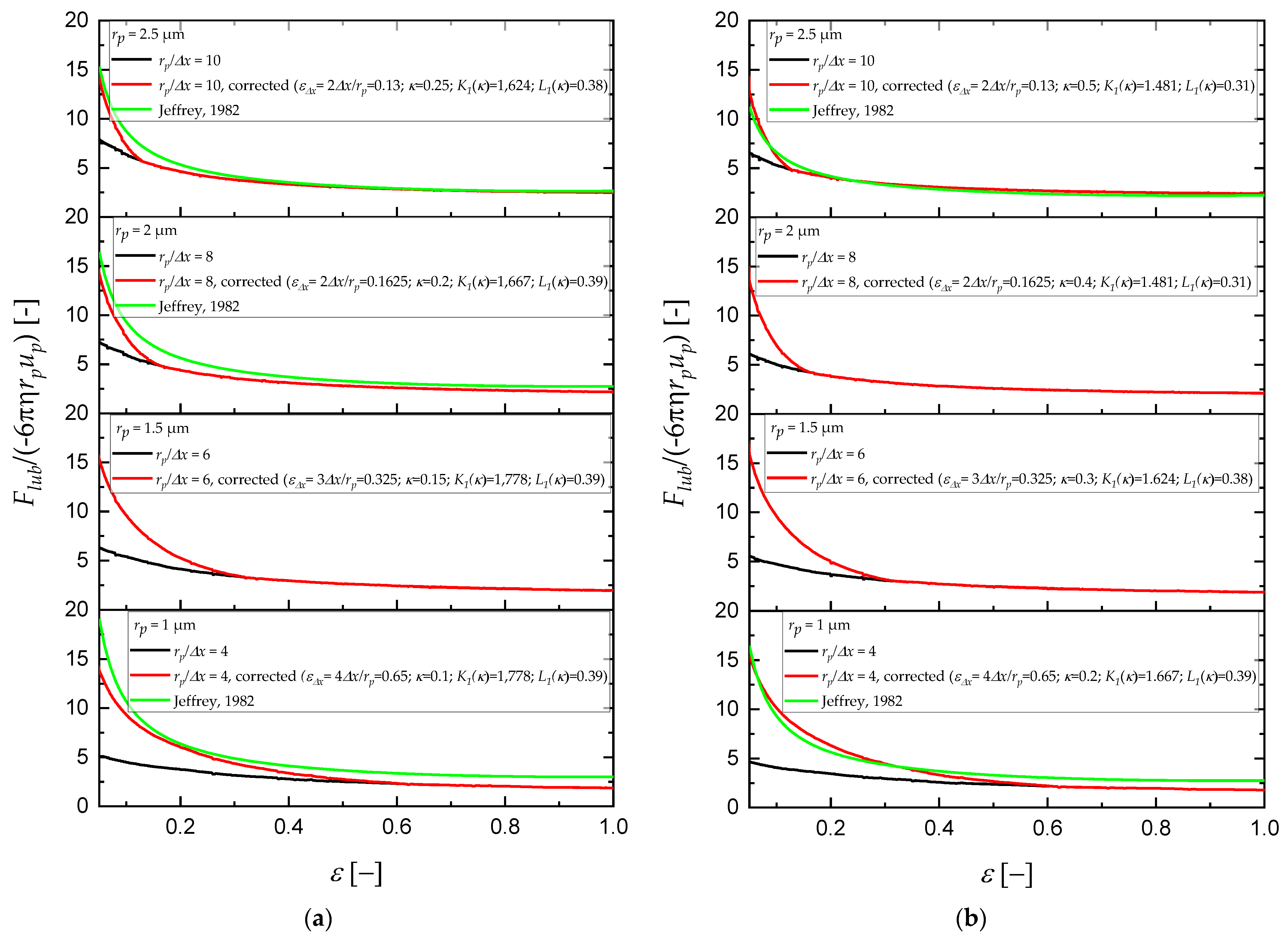
Activation distance for lubrication correctionɛxSee Figure 3(-)
Density of fluidσf1000kg/m3
Kinematic viscosityυ1 × 10⁻⁶m2/s
Publisher’s Note: MDPI stays neutral with regard to jurisdictional claims in published maps and institutional affiliations.

