Enhance Teaching-Learning-Based Optimization for Tsallis-Entropy-Based Feature Selection Classification Approach

Abstract

Feature selection is an effective method to reduce the number of data features, which boosts classification performance in machine learning. This paper uses the Tsallis-entropy-based feature selection to detect the significant feature. Support Vector Machine (SVM) is adopted as the classifier for classification purposes in this paper. We proposed an enhanced Teaching-Learning-Based Optimization (ETLBO) to optimize the SVM and Tsallis entropy parameters to improve classification accuracy. The adaptive weight strategy and Kent chaotic map are used to enhance the optimal ability of the traditional TLBO. The proposed method aims to avoid the main weaknesses of the original TLBO, which is trapped in local optimal and unbalance between the search mechanisms. Experiments based on 16 classical datasets are selected to test the performance of the ETLBO, and the results are compared with other well-established optimization algorithms. The obtained results illustrate that the proposed method has better performance in classification accuracy.

1. Introduction

Machine learning has been widely used in many practical applications such as data mining, text processing, pattern recognition, and medical image analysis, which often rely on large data sets [1,2]. From utilizing label information, feature selection algorithms are mainly categorized as filters or wrapper approaches [3,4]. The wrapper-based methods are commonly used to finish the classification task [5]. The main step includes classifiers, evaluation criteria of features, and finding the optimal features [6].

The SVM algorithm is one of the most popular supervised models and is regarded as one of the most robust methods in the machine learning field [7,8]. SVM has some robust characteristics compared to other methods, such as excellent generalization performance, which is able to generate high-quality decision boundaries based on a small subset of training data points [9]. The largest problems encountered in setting up the SVM model are how to select the kernel function and its parameter values. Inappropriate parameter settings will lead to poor classification results [10].

Swarm intelligence algorithms can solve complex engineering problems, but different optimization algorithms solve different engineering problems with different effects [11,12]. The optimization algorithms can reduce the time and improve the segmentation accuracy. There many optimization algorithms are proposed, such as Genetic Algorithm (GA) [13], Particle Swarm Optimization (PSO) [14], Differential Evolution (DE) [15], Ant Colony Optimization (ACO) [16], Artificial Bee Colony (ABC) algorithm [17], Grey Wolf Optimizer (GWO) [18], Ant Lion Optimizer (ALO) [19], Moth-flame Optimization (MFO) [20], Whale Optimization Algorithm (WOA) [21], Invasive weed optimization algorithm [22], Flower Pollination Algorithm [23]. Although all algorithms have advantages, no-free lunch (NFL) [24] has proved that no algorithm can solve all optimization problems.

There is no perfect optimization algorithm, and the optimization algorithm should be improved to solve engineering problems better. Many scholars study the strategies for improving optimization algorithm. The strategies commonly used by scholars are as follows adaptive weight strategy and chaotic map. Zhang Y. proposed an improved particle swarm optimization algorithm with an adaptive learning strategy [25]. The adaptive learning strategy increased the population diversity of PSO. Dong Z. proposed a self-adaptive weight vector adjustment strategy based on a chain segmentation strategy [26]. The self-adaptive solved the shape of the true Pareto front (PF) of the multi-objective problem. Li E. proposed a multi-objective decomposition algorithm based on adaptive weight vector and matching strategy [27]. The adaptive weight vector solved the degradation of the performance of the solution set. The chaotic map is also a general nonlinear phenomenon, and its behavior is complex and semi-random. It is mathematically defined as the randomness generated by a simple deterministic system [28]. Xu C. proposed an improved boundary bird swarm algorithm [29]. The algorithm combined the good global convergence and robustness of the birds’ swarm algorithm. Tran, N. T. presented a method for fatigue life prediction of 2-DOF compliant mechanism which combined the differential evolution algorithm and the adaptive neuro-fuzzy inference system [30]. The experiment result shows that the accuracy of the proposed method is high.

Teaching-Learning-Based Optimization (TLBO) is proposed by R. V. Rao, which solves the global problem of continuous nonlinear functions [31]. The TLBO approach works on the philosophy of teaching and learning. Many scholars study the strategies to improve the optimization ability for a different problem. Gunji A. B. proposed improved TLBO for solving assembly sequence problems [32]. Zhang H. proposed a hybridizing TLBO [33]. The approach can enable better tracking accuracy and efficiency. Ho, N.L. presented a hybrid Taguchi-teaching learning-based optimization algorithm (HTLBO) [34]. The proposed method had good agreement with the predicted results. The strategies can improve the optimal ability of TLBO. In this paper, for solving the problem of learning efficiency and initial parameter setting, we use several strategies to enhance the optimal ability of the TLBO.

The main contribution of our work includes:

(1)

The enhanced Teaching-Learning-Based Optimization (ETLBO) is proposed to improve optimal ability. The adaptive weight and Kent chaotic map are used to enhance the TLBO. These two strategies can improve the searching ability of the students and teachers in TLBO.

(2)

We adopt the Tsaliis entropy-based feature selection method for finding the crucial feature. The selected feature x and the parameter $\alpha$ of Tsallis entropy are optimized by ETLBO.

(3)

The parameter c of the SVM classifier is optimized by ETLBO for obtaining high classification accuracy. The core idea of this method is to automatically determine the parameter $\alpha$ of Tsallis entropy and parameter c of the SVM under different data.

The proposed method is tested on several feature selection and classification problems in terms of several comment evaluation measures. The results are compared with other well-established optimization methods. The obtained results showed that the proposed ETLBO got better and promising results in almost all the tested problems compared to other methods.

The rest of the paper is described as follows: Section 2 introduces Tsallis’s entropy-based feature selection formula. Section 3, Enhance Teaching-learning-based optimization, and the ETLBO optimizes the feature selection design is introduced. In Section 4 and Section 5, the feature selection results and the algorithm analysis are given. Finally, the conclusions are summarized in Section 6.

2. Related work

2.1. Tsallis Entropy-Based Feature Selection (TEFS)

TEFS estimates the importance of a feature by calculating its information gain (IG) with respect to the target feature. The IG is calculated by subtracting the Tsallis entropy of features concerning target from the total entropy of the target feature. The Tsallis entropy and IG are defined as follow:

$$H(m)=\frac{1}{1-\alpha }\log {\displaystyle \sum _{i=1}^n{p}_i^{\alpha }}$$

(1)

$$IG(m|n)=H(m)-H(m|n)$$

(2)

where, $H(m)$ represents the Tsallis entropy of a feature m, $IG(m|n)$ represents the Tsallis entropy of a target in terms of a feature n, m is the number of target feature, n is the total number of the feature.

IG measures the significance of a feature by calculating how much information a feature obtains us about the target.

2.2. SVM Classifier

SVM finds the optimal separation of hyperplanes between classes by focusing on the training cases of the edges of effectively discarded classes. For training samples $F=\{(x_1,y_1),\dots ,(x_n,y_n)\}$ in different dimensional spaces, a classifier can be accurately summarized. The main core of SVM is finding a suitable kernel function $k(x_i,x_j)=\varphi (x_i)\cdot \varphi (x_j)$, where $\varphi (x_i)$ is a nonlinear function, and the function is used to transfer the nonlinear space of the sample input to two hyperplanes. The formula can be written as:

$$f(x)=w\cdot \varphi (x)+b$$

(3)

where, $w$ is the weight vector, $b$ is the threshold value, and $(\cdot )$ represents the inner product operation. The objective of SVM is to determine the $w$, and $b$ when minimizing the $w^{T}w/2$, it can be seen below:

$$\min \frac{1}{2}\Vert w\Vert +C{\displaystyle \sum _{i=1}^n{\xi }_i}$$

(4)

where, ${\xi }_i$ is the slack variable, C is the penalty parameter.

The most commonly used kernel is the Gaussian kernel, used for data conversion in SVM. The Gaussian kernel is defined as:

$$K(x_i,x_j)=\exp (-\frac{{\Vert x_i-x_j\Vert }^2}{2{\delta }^2})$$

(5)

where, $\delta >0$ denotes the width parameter, and δ controls the mapping results.

The strategy of reducing multi-class problems to a set of dichotomies enables support vector machines to be used more appropriately with fewer computational requirements, that is, to consider all classes at once and thus to obtain a multi-class support vector machine. One way to do this is by solving a single optimization problem, similar to the “one for all” approach on a fundamental basis. There are n decision functions or hyperplanes, and the problems can convert to one problem as:

$$\min \frac{1}{2}{\displaystyle \sum _{i=1}^n{w}_i^T{w}_i}+C{\displaystyle \sum _{j=1}^m{\displaystyle \sum _{i\ne y_j}{\xi }_j^i{w}_{y_j}^T\phi (x_j)}}+b_{y_j}$$

(6)

where, ${\xi }_j^i\ge 0$. The resulting decision function can be represented as:

$$\arg {\max }_i(w_i^T\phi (x_i)+b_i)$$

(7)

2.3. Fitness Function Design

The main indexes influencing FS are the classification error accuracy and the number of features. So, how to balance the number of features and the classification is the essential key for the FS problem. Whereas, $f_1$ is the Normalized Mutual Information (NMI) [13]. The formula can be seen as follow:

$$f_1(x)=NMI(X,S)=\frac{MI(X;S)}{[G(X)+G(S)]/2}$$

(8)

where, X is the set of clusters and S is the set of classes. The MI is the mutual information between X and S [35]. It can be defined as follow:

$$\begin{array}{ll}MI(X;S)& ={\displaystyle \sum _k}{\displaystyle \sum _j}P\left(X_k\cap S_j\right)\log \frac{P\left(X_k\cap S_j\right)}{P\left(X_k\right)P\left(S_j\right)}\\ & ={\displaystyle \sum _k}{\displaystyle \sum _j}\frac{\left|X_k\cap S_j\right|}{N}\log \frac{N\left|X_k\cap S_j\right|}{\left|X_k\right|\left|S_j\right|}\end{array}$$

(9)

where, $P(X_k)$, $P(S_j)$, $P\left(X_k\cap S_j\right)$ is the probability of the $X_k$, $S_j$, and $X_k\cap S_j$. The $G(X)$ comes from the maximum likelihood estimation of probability.

$$\begin{array}{ll}G(X)& =-{\displaystyle \sum _k}P\left(X_k\right)\log P\left(X_k\right)\\ & =-{\displaystyle \sum _k}\frac{\left|X_k\right|}{N}\log \frac{\left|X_k\right|}{N}\end{array}$$

(10)

3. Enhance Teaching-Learning-Based Optimization (ETLBO)

In this section, we introduce the proposed method in detail. Firstly, we introduce the TLBO and the strategies used in the proposed method. And then, the ETLBO is introduced. Finally, the flowchart of the proposed method is described.

3.1. Teacher Phase

It is the first part of the algorithm where the learner with the highest marks acts as a teacher, and the teacher’s task is to increase the mean marks of the class. The update process of i-th learner in teacher phase is formulated as:

$$X_{i,new}=X_i+rand\times (X_{teacher}-T_F\times X_{ave})$$

(11)

where, $X_i$ is the solution of the i-th learner, $X_{teacher}$ represents the teacher’s solution, $X_{ave}$ means the average of all learners, rand is a random number in (0,1), and $T_F$ is the teaching factor that decides the value of mean to be changed. The value can be either 1 or 2, which is again a heuristic step and decided randomly with equal probability $T_F=round[1+rand(0,1)\{2-1\}]$.

In addition, the new solution $X_{i,new}$ is accepted only if it is better than the previous solution, it can be formulated as:

$$X_i=\{\begin{array}{l}{X}_{i,new}\begin{array}{cc}f(X_{i,new})>f(X_i)& \end{array}\\ X_i\begin{array}{ccc}& otherwise& \end{array}\end{array}$$

(12)

where, f means the fitness function.

3.2. Learner Phase

The second part of the algorithm is where the learner updates its knowledge through interaction with other learners. In each iteration, two learners interact with $X_m$ and $X_n$, in which the more innovative learner improves the marks of other learners. In the learner phase, one learner learns new things if the other learner has more knowledge than himself. The phenomenon is described as follows:

$$X_{m,new}=\{\begin{array}{l}{X}_m+rand\times (X_m-X_n);f(X_m)>f(X_n)\\ X_m+rand\times (X_n-X_m);f(X_n)>f(X_m)\end{array}$$

(13)

The temporary solution is accepted only if it is better than the previous solution; it can be formulated as:

$$X_m=\{\begin{array}{l}{X}_{m,new};f(X_{m,new})>f(X_m)\\ X_m;otherwise\end{array}$$

(14)

3.3. Adaptive Weight Strategy

The adaptive weight strategy is easier to jump out of local minima, facilitating global optimization. While the TLBO solves the problem of the complex optimized function, the algorithm will easily fall into the local optimum. And a smaller inertia factor is beneficial for precise local search for the current search domain. We design a new weight strategy t which can be written as follows:

$$t={(1-\frac{iter}{Max\_iter})}^{1-\sin (\pi \frac{iter}{Max\_iter})}$$

(15)

where, iter is the current number of the iteration; Max_iter is the max number of the iteration.

3.4. Kent Chaotic Map (KCM)

Chaotic mapping is one kind of nonlinear mapping that can generate a random number sequence. It is sensitive to initial values, which ensures that the encoder can generate an unrelated encoding sequence. There are many kinds of chaotic maps, such as Logistic map, Kent map, etc. In this paper, we use the Kent map as the improved strategy. The formula of the Kent map can be seen as follow:

$$f(x)=\{\begin{array}{l}\frac{x}{a}\begin{array}{cc}\begin{array}{cc}& \end{array}& 0<x\le a\end{array}\\ \frac{1-x}{1-a}\begin{array}{cc}& a<x<1\end{array}\end{array}$$

(16)

where, a is a variable value, x is the initial value of the $x(0)$. In this paper, $a=0.5$.

3.5. Proposed Method

There are two phases in the basic TLBO search process to update the individual’s position. In the teacher phase, we use the Kent chaotic map to improve the original state of the teacher. The teacher can be endowed with different abilities to teach the different students. This strategy allows the abilities of different teachers to be demonstrated. In the learner phase, we design a learning efficiency to improve the students’ learning state. The adaptive weight strategy can improve itself with the iteration increases. The students will learn more knowledge at the beginning phase of the iteration. The students can obtain enough knowledge at the end of the iteration, and the adaptive weight gets small. The students can learn the different knowledge at the different phases. The formula can be represented as follow:

$$X_{m,new}=\{\begin{array}{l}{X}_m\times t+rand\times (X_m-X_n);f(X_m)>f(X_n)\\ X_m\times t+rand\times (X_n-X_m);f(X_n)>f(X_m)\end{array}$$

(17)

where, t is the adaptive weight.

The proposed classification method can be divided into two parts: feature selection and the parameter selection of the SVM. At first, the Tsallis entropy of the target is calculated using Equation (1). Then the entropy of each feature concerning the target is calculated and subtracted from the target’s entropy using Equation (2). In this process, the selected feature x and the parameter $\alpha$ of Tsallis entropy are optimized by the ETLBO. The parameter $\alpha$ can decide the ability of the Tsallis entropy.

In the second part, we use the ETLBO to optimize parameter c of SVM. The penalty coefficient c is the compromise between the smoothness of the fitting function and the classification accuracy. When c is too large, the training accuracy is high, and the generalization ability is poor; while c is too small, errors will be increased. Therefore, a reasonable selection of parameter c can obviously improve the model’s classification accuracy and generalization ability.

Finally, the selected feature x, the parameter $\alpha$ of Tsallis entropy, and the parameter c of SVM are optimized by ETLBO. We use the parameter optimized by the ETLBO and the SVM to classify the test dataset. The SVM classifier output the classification result. The flowchart of the proposed method is shown in Figure 1.

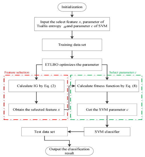
Figure 1. The flowchart of the proposed method.

4. Experiment and Result

To analysis the effectiveness of the proposed method, five optimization algorithms are used for comparison, such as PSO [13], WOA [20], HHO [36], TLBO [29], HSOA [37], and HTLBO [34]. The PSO, WOA, HHO, and TLBO are the original optimization algorithms. These optimization algorithms have the strong ability to find the optimal value of the mathematical function. While these algorithms optimize the engineering problems, the optimization performance is not well. Many schoolers study the strategies to improve the optimization algorithms. The HSOA and HTLBO are improved methods. These two algorithms use the hybrid way to enhance the optimization ability of the SOA and TLBO. The improved methods have the excellent performance to solve the problems which mentioned in the reference [34,37]. However, these algorithms may not solve all problems. Therefore, we select these algorithms as compared algorithms to test the performance of the proposed method.

The set of parameters is the same as the reference. All the methods are coded and implemented in MATLAB 2018B. To keep the fairness of the compared algorithms, each algorithm runs 30 times independently. To test the performance of the comparison algorithm, we set the number of populations to 30 and the maximum iteration to 500. The proposed ETLBO is training in MATLAB2018B. Experiments are managed on a computer with an i7-11800H central processing unit.

The results of the proposed method are described in this section. First, the fitness values obtained by the different optimization algorithms are compared to show the performances of these approaches. Then, we analyze the classification result of the compared algorithms. Finally, the discussion of the proposed method is described.

4.1. Datasets and Evaluation Index

The benchmark datasets used in the evaluations are introduced. The dataset selects 16 standard datasets from the University of California (UCI) data repository [38]. Table 1 records the primary information of these selected datasets.

Table 1. The datasets used in the experiments.

	Datasets	Samples	Features
1	Iris	150	4
2	Wine	178	13
3	Sonar	208	60
4	Vehicle	846	18
5	Balancescale	625	4
6	CMC	1473	9
7	Cancer	683	9
8	Vowel	871	3
9	Thyroid	215	5
10	WDBC	569	30
11	HeartEW	270	13
12	Lymphography	148	18
13	SonarEW	208	60
14	IonosphereEW	351	34
15	Vote	300	16
16	WaveformEW	5000	40

To evaluate the result of the health index diagnosis, we use the F-score, the accuracy of the classification and the CPU time as the metric index.

The function of F-score can be defined as follow:

$$F-score=(1+{\beta }^2)\cdot \frac{Precision\cdot Recall}{{\beta }^2\cdot Precision+Recall}$$

(18)

$$Precision=\frac{Tp}{Tp+Fp}$$

(19)

$$Recall=\frac{Tp}{Tp+Fn}$$

(20)

where, $Tn$ is the number of negative classes, $Fn$ is the number of negative classes, $Tp$ is the number of positive classes, and $Fp$ is the number of positive classes.

4.2. Experiment 1: Feature Selection

Table 2 shows the fitness value of the compared algorithms. The table shows that when the number of features is small, the compared algorithms can reduce the number of features. When the number of features increases, it takes a huge challenge for the optimization algorithms. The ETLBO obtains better performance than compared algorithms. Table 3 shows the std of the fitness values. It can be known from the given table that the ETLBO has strong robustness.

Table 2. The fitness values of compared algorithms.

	PSO	WOA	HHO	TLBO	HSOA	HTLBO	ETLBO
Iris	0.0271	0.0271	0.0271	0.0271	0.0271	0.0271	0.0271
Wine	0.1846	0.1657	0.1594	0.1709	0.1585	0.1576	0.1521
Sonar	0.2655	0.2147	0.2356	0.2386	0.2268	0.2258	0.2145
Vehicle	0.2972	0.2575	0.2746	0.2528	0.2432	0.2741	0.2716
Balancescale	0.0619	0.0519	0.0540	0.0613	0.0521	0.0556	0.0516
CMC	0.1937	0.1855	0.1837	0.1777	0.1701	0.1758	0.1621
Cancer	0.0629	0.0710	0.0660	0.0645	0.0634	0.0645	0.0612
Vowel	0.1251	0.1251	0.1251	0.1251	0.1251	0.1251	0.1251
Thyroid	0.0934	0.0853	0.0995	0.0922	0.0925	0.0921	0.0851
WDBC	0.3828	0.3155	0.3678	0.3258	0.3234	0.3221	0.3154
HeartEW	0.2942	0.2993	0.3325	0.2869	0.3077	0.2989	0.2814
Lymphography	0.2208	0.2040	0.2127	0.1965	0.1999	0.1989	0.1951
SonarEW	0.3650	0.4065	0.3892	0.3721	0.3610	0.3589	0.3514
IonosphereEW	0.3390	0.3425	0.3718	0.3339	0.3426	0.3411	0.3226
Vote	0.2274	0.2567	0.2460	0.2542	0.2215	0.2218	0.2158
WaveformEW	0.4348	0.4151	0.3998	0.4436	0.4278	0.4025	0.3915

Table 3. The std of fitness values.

	PSO	WOA	HHO	TLBO	HSOA	HTLBO	ETLBO
Iris	4.56 × 10−4	4.69 × 10−4	5.40 × 10−4	4.60 × 10−4	4.86 × 10−4	4.88 × 10−4	4.50 × 10−4
Wine	6.84 × 10−4	6.53 × 10−4	6.07 × 10−4	6.22 × 10−4	5.79 × 10−4	5.82 × 10−4	5.60 × 10−4
Sonar	1.27 × 10−4	1.12 × 10−5	1.00 × 10−5	1.08 × 10−5	1.10 × 10−5	1.11 × 10−5	1.00 × 10−5
Vehicle	6.54 × 10−4	6.16 × 10−4	6.37 × 10−4	6.95 × 10−4	6.13 × 10−4	6.15 × 10−4	6.10 × 10−4
Balancescale	4.25 × 10−4	4.49 × 10−4	4.50 × 10−4	4.89 × 10−4	4.17 × 10−4	4.20 × 10−4	4.10 × 10−4
CMC	4.13 × 10−4	3.47 × 10−4	3.96 × 10−4	3.56 × 10−4	3.40 × 10−4	3.41 × 10−4	3.30 × 10−4
Cancer	1.15 × 10−3	1.13 × 10−3	1.03 × 10−3	1.03 × 10−3	1.02 × 10−3	1.02 × 10−4	9.60 × 10−4
Vowel	7.80 × 10−4	7.68 × 10−4	8.44 × 10−4	7.94 × 10−4	7.74 × 10−4	7.78 × 10−4	7.50 × 10−4
Thyroid	6.82 × 10−4	6.79 × 10−4	7.33 × 10−4	7.22 × 10−4	7.26 × 10−4	7.26 × 10−4	6.70 × 10−4
WDBC	1.05 × 10−3	1.01 × 10−3	1.02 × 10−3	1.01 × 10−3	9.74 × 10−4	9.78 × 10−4	9.40 × 10−4
HeartEW	9.67 × 10−4	9.34 × 10−4	9.08 × 10−4	1.00 × 10−3	8.91 × 10−4	8.93 × 10−4	8.80 × 10−4
Lymphography	8.62 × 10−4	7.11 × 10−4	8.00 × 10−4	8.13 × 10−4	7.44 × 10−4	7.47 × 10−4	6.90 × 10−4
SonarEW	4.54 × 10−4	3.81 × 10−4	3.91 × 10−4	4.50 × 10−4	4.00 × 10−4	4.02 × 10−4	3.80 × 10−4
IonosphereEW	9.56 × 10−4	8.85 × 10−4	8.22 × 10−4	7.72 × 10−4	7.82 × 10−4	7.88 × 10−4	7.40 × 10−4
Vote	8.81 × 10−4	9.30 × 10−4	9.87 × 10−4	9.64 × 10−4	9.23 × 10−4	9.25 × 10−1	8.50 × 10−4
WaveformEW	4.34 × 10−4	4.51 × 10−4	4.28 × 10−4	4.34 × 10−4	3.92 × 10−4	3.93 × 10−4	3.90 × 10−4

Table 4 shows the number of the selected attributes. The compared algorithms can reduce the number of features. The attributes are little, and the compared algorithms obtain the same result. The ETLBO gets the least attributes among the compared algorithms when the attributes are large. The total attributes of the dataset, the ETLBO also obtain the least attributes than other algorithms. It means that the ETLBO can reduce the number of features. However, reducing the number of features does not mean the classification accuracy is high.

Table 4. The average number of selected attributes.

	Attributes	PSO	WOA	HHO	TLBO	HSOA	HTLBO	ETLBO
Iris	4	3	3	3	3	3	3	3
Wine	13	6	6	5	10	6	6	5
Sonar	60	31	32	32	48	29	29	28
Vehicle	18	4	4	4	4	4	4	4
Balancescale	4	4	3	4	4	4	3	3
CMC	9	7	6	6	8	7	8	6
Cancer	9	5	6	5	7	6	6	5
Vowel	3	3	3	3	3	3	3	3
Thyroid	5	4	4	3	4	4	4	3
WDBC	30	9	8	7	10	7	8	6
HeartEW	13	5	5	4	6	5	5	4
Lymphography	18	6	7	7	6	8	6	5
SonarEW	60	19	18	19	22	15	13	12
IonosphereEW	34	25	23	20	17	15	14	12
Vote	16	8	7	9	8	6	6	6
WaveformEW	40	21	26	24	23	20	18	16
Total	336	160	161	155	183	142	136	121

Table 5 shows the parameter obtained by ETLBO. It can be seen from the table that the ETBLO obtains the different values under the diverse dataset. The ETBLO not only reduce the number of features but also acquires the parameter α of Tsallis entropy and the parameter c of SVM. We will test the performance of the compared algorithms in the next section.

Table 5. The parameter obtained by ETLBO.

	$\mathit{\alpha }$	c
Iris	0.52	1.14
Wine	0.64	1.20
Sonar	0.80	1.24
Vehicle	0.22	1.83
Balancescale	0.77	1.17
CMC	0.26	1.22
Cancer	0.15	0.65
Vowel	0.07	1.82
Thyroid	0.61	1.01
WDBC	0.81	1.17
HeartEW	0.78	0.95
Lymphography	0.47	1.64
SonarEW	0.08	1.82
IonosphereEW	0.55	0.99
Vote	0.73	1.58
WaveformEW	0.55	0.73
Total	0.73	1.83

4.3. Experiment 2: Classification

Table 6 shows the classification results of compared algorithms. Table 7 shows the f-score of the compared methods. The table result shows that the ETLBO is better than the original TLBO. The strategies improve the optimal ability of the TLBO. At the same time, the HSOA and ETLBO are better than the other algorithms. It means that the strategies significantly boost the original optimization algorithms. It can be known that the methods can be ordered as follows in terms of them F-score result: ETLBO > HTLBO > HSOA > HHO > PSO > WOA > TLBO. To sum up, the ETLBO obtains the high f-score values.

Table 6. The classification accuracy of compared algorithms.

	PSO	WOA	HHO	TLBO	HSOA	HTLBO	ETLBO
Iris	0.9545	0.9481	0.9320	0.9167	0.9548	0.9546	0.9579
Wine	0.9413	0.9303	0.9232	0.9369	0.9411	0.9479	0.9488
Sonar	0.9160	0.9375	0.9242	0.9025	0.9347	0.9359	0.9435
Vehicle	0.9012	0.9306	0.9147	0.9358	0.9345	0.9339	0.9414
Balancescale	0.9338	0.9241	0.9308	0.9287	0.9450	0.9442	0.9465
CMC	0.9440	0.9271	0.9259	0.9253	0.9387	0.9371	0.9454
Cancer	0.9060	0.9180	0.9403	0.9356	0.9349	0.9408	0.9438
Vowel	0.9600	0.9477	0.9429	0.9559	0.9628	0.9581	0.9651
Thyroid	0.9031	0.9249	0.9048	0.8849	0.9202	0.9282	0.9285
WDBC	0.9329	0.9351	0.9177	0.9057	0.9345	0.9358	0.9385
HeartEW	0.9230	0.9118	0.9143	0.8995	0.9323	0.9271	0.9358
Lymphography	0.9022	0.9256	0.9001	0.9141	0.9210	0.9180	0.9268
SonarEW	0.9360	0.9115	0.9116	0.9164	0.9336	0.9357	0.9361
IonosphereEW	0.9361	0.9448	0.9276	0.9233	0.9384	0.9441	0.9458
Vote	0.9136	0.9170	0.9217	0.9008	0.9381	0.9378	0.9451
WaveformEW	0.9276	0.9354	0.9229	0.9029	0.9292	0.9284	0.9365

Table 7. The f-score of compared algorithms.

	PSO	WOA	HHO	TLBO	HSOA	HTLBO	ETLBO
Iris	0.9362	0.9038	0.9193	0.9007	0.9262	0.9334	0.9498
ine	0.9118	0.9116	0.9175	0.9219	0.9194	0.9288	0.9433
Sonar	0.9043	0.913	0.9206	0.8754	0.9223	0.9091	0.9359
Vehicle	0.8782	0.8895	0.9038	0.9142	0.918	0.9164	0.9387
Balancescale	0.9169	0.9055	0.9139	0.9139	0.9309	0.9276	0.9422
CMC	0.9295	0.9	0.8988	0.8977	0.9217	0.9109	0.9429
Cancer	0.8861	0.9119	0.8945	0.9104	0.9133	0.9223	0.9396
Vowel	0.9399	0.914	0.9336	0.9345	0.9464	0.9506	0.9601
Thyroid	0.8812	0.8759	0.8954	0.8585	0.908	0.904	0.9211
WDBC	0.9102	0.9039	0.9071	0.8913	0.9128	0.9143	0.9329
HeartEW	0.8936	0.8887	0.8962	0.8892	0.9045	0.9186	0.9275
Lymphography	0.8894	0.8725	0.9117	0.8891	0.8883	0.9109	0.9184
SonarEW	0.9199	0.8988	0.897	0.8888	0.9066	0.9092	0.9360
IonosphereEW	0.9171	0.9088	0.9212	0.9090	0.9304	0.9168	0.9411
Vote	0.8890	0.9108	0.9057	0.8776	0.9225	0.9204	0.9449
WaveformEW	0.9115	0.8948	0.9106	0.8888	0.9089	0.9102	0.9346

To sum up, the ETLBO obtained the best result in compared algorithms. The ETLBO not only reduces the number of features but also obtains high classification accuracy. Table 8 shows that the std of classification accuracy. The ETLBO has a better stable ability than other algorithms. The proposed method has strong robustness to finish the classification task.

Table 8. The std of classification accuracy.

	PSO	WOA	HHO	TLBO	HSOA	HTLBO	ETLBO
Iris	4.57 × 10−5	4.69 × 10−5	5.45 × 10−5	4.63 × 10−5	4.90 × 10−5	4.60 × 10−5	4.54 × 10−5
Wine	6.87 × 10−5	6.56 × 10−5	6.08 × 10−5	6.22 × 10−5	5.84 × 10−5	6.90 × 10−5	5.65 × 10−5
Sonar	1.28 × 10−6	1.12 × 10−5	1.01 × 10−6	1.08 × 10−5	1.10 × 10−6	1.28 × 10−6	1.00 × 10−5
Vehicle	6.60 × 10−5	6.19 × 10−5	6.39 × 10−5	6.98 × 10−5	6.14 × 10−5	6.63 × 10−5	6.12 × 10−5
Balancescale	4.28 × 10−5	4.50 × 10−5	4.52 × 10−5	4.92 × 10−5	4.18 × 10−5	4.31 × 10−5	4.13 × 10−5
CMC	4.14 × 10−5	3.50 × 10−5	3.97 × 10−5	3.58 × 10−5	3.41 × 10−5	4.18 × 10−5	3.32 × 10−5
Cancer	1.15 × 10−4	1.14 × 10−4	1.03 × 10−4	1.04 × 10−4	1.02 × 10−4	1.16 × 10−5	9.62 × 10−5
Vowel	7.80 × 10−5	7.69 × 10−5	8.48 × 10−5	7.98 × 10−5	7.78 × 10−5	7.88 × 10−5	7.55 × 10−5
Thyroid	6.86 × 10−5	6.83 × 10−5	7.39 × 10−5	7.28 × 10−5	7.33 × 10−5	6.88 × 10−5	6.74 × 10−5
WDBC	1.06 × 10−4	1.01 × 10−4	1.02 × 10−4	1.02 × 10−4	9.84 × 10−5	1.06 × 10−5	9.42 × 10−5
HeartEW	9.76 × 10−5	9.43 × 10−5	9.11 × 10−5	1.00 × 10−4	8.95 × 10−5	9.86 × 10−5	8.86 × 10−5
Lymphography	8.70 × 10−5	7.18 × 10−5	8.07 × 10−5	8.16 × 10−5	7.50 × 10−5	8.73 × 10−5	6.94 × 10−5
SonarEW	4.55 × 10−5	3.84 × 10−5	3.92 × 10−5	4.51 × 10−5	4.02 × 10−5	4.56 × 10−5	3.81 × 10−5
IonosphereEW	9.61 × 10−5	8.88 × 10−5	8.24 × 10−5	7.74 × 10−5	7.87 × 10−5	9.66 × 10−5	7.45 × 10−5
Vote	8.82 × 10−5	9.35 × 10−5	9.97 × 10−5	9.64 × 10−5	9.31 × 10−5	8.89 × 10−5	8.56 × 10−5
WaveformEW	4.38 × 10−5	4.55 × 10−5	4.29 × 10−5	4.35 × 10−5	3.94 × 10−5	4.41 × 10−5	3.92 × 10−5

A statistical test is an essential and vital measure to evaluate and prove the performance of the tested methods. Parameter statistical test is based on various assumptions. This section uses well-known non-parametric statistical test types, Wilcoxon’s rank-sum test [39]. Table 9 shows the results of the Wilcoxon rank-sum test. It can be found that the ETLBO is significantly different from other methods.

Table 9. Wilcoxon’s rank-sum test of classification accuracy.

	PSO		WOA		HHO		TLBO		HSOA		HTLBO
	p-Value	h	p-Value	h	p-Value	h	p-Value	h	p-Value	h	p-Value	h
Iris	<0.05	1	<0.05	1	<0.05	1	<0.05	1	<0.05	1	<0.05	1
Wine	<0.05	1	<0.05	1	<0.05	1	<0.05	1	<0.05	1	<0.05	1
Sonar	<0.05	1	<0.05	1	<0.05	1	<0.05	1	<0.05	1	<0.05	1
Vehicle	<0.05	1	<0.05	1	<0.05	1	<0.05	1	<0.05	1	<0.05	1
Balancescale	<0.05	1	<0.05	1	<0.05	1	<0.05	1	<0.05	1	<0.05	1
CMC	<0.05	1	<0.05	1	<0.05	1	<0.05	1	<0.05	1	<0.05	1
Cancer	<0.05	1	<0.05	1	<0.05	1	<0.05	1	<0.05	1	<0.05	1
Vowel	<0.05	1	<0.05	1	<0.05	1	<0.05	1	<0.05	1	<0.05	1
Thyroid	<0.05	1	<0.05	1	<0.05	1	<0.05	1	<0.05	1	<0.05	1
WDBC	<0.05	1	<0.05	1	<0.05	1	<0.05	1	<0.05	1	<0.05	1
HeartEW	<0.05	1	<0.05	1	<0.05	1	<0.05	1	<0.05	1	<0.05	1
Lymphography	<0.05	1	<0.05	1	<0.05	1	<0.05	1	<0.05	1	<0.05	1
SonarEW	<0.05	1	<0.05	1	<0.05	1	<0.05	1	<0.05	1	<0.05	1
IonosphereEW	<0.05	1	<0.05	1	<0.05	1	<0.05	1	<0.05	1	<0.05	1
Vote	<0.05	1	<0.05	1	<0.05	1	<0.05	1	<0.05	1	<0.05	1
WaveformEW	<0.05	1	<0.05	1	<0.05	1	<0.05	1	<0.05	1	<0.05	1

The CPU time is also an important index for the practical engineering testing problem. The CPU time results of the compared algorithms can be seen in Table 10. The CPU time ordering of each algorithm is: TLBO < PSO < WOA < HHO < ETLBO < HTLBO < HSOA. Although the ETLBO costs considerable CPU time, the classification accuracy has good performance. At the same time, the ETLBO uses less CPU time than HSOA. It means that the strategies have good adaptive effectiveness for the TLBO. The strategies enhance the TLBO under less CPU time than the improved method.

Table 10. The CPU time of the compared algorithms.

	ETLBO	PSO	WOA	HHO	TLBO	HSOA	HTLBO
Iris	2.3973	1.8441	2.0285	2.1794	1.6764	2.637	2.4128
Wine	4.1247	3.1729	3.4902	3.7498	2.8844	4.5372	4.1315
Sonar	6.65	5.1154	5.6269	6.0454	4.6503	7.315	6.6542
Vehicle	4.1722	3.2094	3.5303	3.7929	2.9176	4.5894	4.1765
Balancescale	2.4302	1.8694	2.0563	2.2093	1.6994	2.6732	2.4462
CMC	3.0792	2.3686	2.6055	2.7993	2.1533	3.3872	3.0803
Cancer	1.5509	1.193	1.3123	1.41	1.0846	1.706	1.5669
Vowel	3.6988	2.8452	3.1298	3.3626	2.5866	4.0687	3.7183
Thyroid	3.6676	2.8212	3.1034	3.3342	2.5648	4.0344	3.6827
WDBC	6.4025	4.925	5.4175	5.8204	4.4772	7.0427	6.4075
HeartEW	4.5164	3.4741	3.8215	4.1058	3.1583	4.968	4.5271
Lymphography	6.4656	4.9735	5.4709	5.8778	4.5214	7.1122	6.4850
SonarEW	6.9375	5.3365	5.8702	6.3068	4.8514	7.6313	6.9569
IonosphereEW	7.552	5.8092	6.3901	6.8654	5.2811	8.3072	7.5664
Vote	5.5987	4.3067	4.7374	5.0898	3.9152	6.1586	5.6065
WaveformEW	3.3821	2.6016	2.8618	3.0746	2.3651	3.7203	3.3848

4.4. Experiment 3: Compared with Different Classifiers

In this section, we compare with the different classifiers. The compared classifiers contain K-NearestNeighbor (KNN), original SVM, and random forest (RF) [40]. Table 11 shows the configuration parameters and characteristics of the classifier models.

Table 11. Configuration parameters and characteristics of the classifier models.

Classifier	Caret Method Value	R Package	Tuning Parameters	Characteristics
KNN	knn		k-5	Unique classifier. The number of neighbors is directly compared to the test data using the KNN function in the Caret package.
SVM	svmRadial	E1071	Σ−7 × 10−2 c-1	Radial basic function outperformed linear SVM.
RF	rf	randomForest	mtry-8 ntree-150	Overcomes the disadvantage of simple DT using a large number of DT’s to classify by majority vote. Use the randomForest function.

Table 12 demonstrates the evaluation index of the compare algorithsm. The BTLBO obtains the best result than other compared classifiers in all index. The BTLBO outperforms KNN, SVM, and RF by yielding an improvement of 3.45%, 2.94%, and 1.62% in F-score index. To sum up, the optimization algorithms obtain the optimal parameter of the SVM. The classification accuracy is higher than other compared classifiers.

Table 12. The evaluation index of compared algorithms.

Classifier	Ac	Pc	R	F-Score
KNN	0.9275	0.9135	0.9123	0.9097
SVM	0.9241	0.9178	0.9167	0.9142
RF	0.9352	0.9189	0.9197	0.9261
BTLBO	0.9478	0.9455	0.9427	0.9411

5. Discussion

The proposed method has an optimal ability to solve the Tsallis-entropy-based feature selection problem in the feature selection domain. The ETLBO selects the suitable parameter of the Tsallis-entropy. At the same time, the proposed method reduces the number of features successfully. The optimization algorithms have a robust optimal ability; however, they do not adapt to solve the different optimized problems. So some adaptive strategies are very effective for improving themselves.

The proposed method obtains better classification accuracy than the compared algorithms in the classification field. The proposed method finds the proper parameter $\alpha$ of the SVM classifier. The proposed method has a higher classification accuracy and strong robustness than the compared algorithms. At the same time, the proposed method is better than orther compared classifiers. So, the ETLBO algorithms can be used in the classification task field.

The proposed method’s limitation is that the optimization algorithm needs iteration to find the optimal solution, which is time-consuming. Improving the optimization capability and reducing the number of iterations can solve this problem. Therefore, it is necessary to search for powerful optimization algorithms and new strategies in future work.

6. Conclusions

In this paper, an enhanced teaching-learning-based optimization is proposed. The adaptive weight strategy and Kent chaotic map are used to enhance the TLBO. The ETLBO optimizes the selected feature x, the parameter $\alpha$ of Tsallis entropy, and the parameter c of SVM. The proposed method reduces the number of features through the UCI data experiment and finds the critical features for classification. Finally, the classification accuracy of the proposed method is better than compared algorithms.

We will design an effective and useful function to reduce the number of features in future work. We will focus on solving the randomness of the TLBO and obtaining more stability parameters of the fitness function. At the same time, we will also test the novel strategies to boost the TLBO.

References

- Ji, B.; Lu, X.; Sun, G.; Zhang, W.; Li, J.; Xiao, Y. Bio-inspired feature selection: An improved binary particle swarm optimization approach. IEEE Access 2020, 8, 85989–86002. [Google Scholar] [CrossRef]
- Kumar, S.; Tejani, G.G.; Pholdee, N.; Bureerat, S. Multiobjecitve structural optimization using improved heat transfer search. Knowl.-Based Syst. 2021, 219, 106811. [Google Scholar] [CrossRef]
- Sun, L.; Wang, L.; Ding, W.; Qian, Y.; Xu, J. Feature selection using fuzzy neighborhood entropy-based uncertainty measures for fuzzy neighborhood multigranulation rough sets. IEEE Trans. Fuzzy Syst. 2020, 99, 1–14. [Google Scholar] [CrossRef]
- Zhao, J.; Liang, J.; Dong, Z.; Tang, D.; Liu, Z. NEC: A nested equivalence class-based dependency calculation approach for fast feature selection using rough set theory. Inform. Sci. 2020, 536, 431–453. [Google Scholar] [CrossRef]
- Liu, H.; Zhao, Z. Manipulating data and dimension reduction methods: Feature selection. In Encyclopedia Complexity Systems Science; Springer: New York, NY, USA, 2009; pp. 5348–5359. [Google Scholar]
- Al-Tashi, Q.; Said, J.A.; Helmi, M.R.; Seyedali, M.; Hitham, A. Binary optimization using hybrid grey wolf optimization for feature selection. IEEE Access 2019, 7, 39496–39508. [Google Scholar] [CrossRef]
- Homayoun, H.; Mahdi, J.; Xinghuo, Y. An opinion formation based binary optimization approach for feature selection. Phys. A Stat. Mech. Its Appl. 2018, 491, 142–152. [Google Scholar]
- Mafarja, M.M.; Mirjalili, S. Hybrid whale optimization algorithm with simulated annealing for feature selection. Neurocomputing 2017, 260, 302–312. [Google Scholar] [CrossRef]
- Aljarah, L.; Ai-zoubl, A.M.; Faris, H.; Hassonah, M.A.; Mirjalili, S.; Saadeh, H. Simultaneous feature selection and support vector machine optimization using the grasshopper optimization algorithm. Cogn. Comput. 2018, 2, 1–18. [Google Scholar] [CrossRef] [Green Version]
- Lin, S.; Ying, K.; Chen, S.; Lee, Z. Particle swarm optimization for parameter determination and feature selection of support vector machines. Expert Syst. Appl. 2008, 35, 1817–1824. [Google Scholar] [CrossRef]
- Sherpa, S.R.; Wolfe, D.W.; Van Es, H.M. Sampling and data analysis optimization for estimating soil organic carbon stocks in agroecosystems. Soil Sci. Soc. Am. J. 2016, 80, 1377. [Google Scholar] [CrossRef]
- Lee, H.M.; Yoo, D.G.; Sadollah, A.; Kim, J.H. Optimal cost design of water distribution networks using a decomposition approach. Eng. Optim. 2016, 48, 16. [Google Scholar] [CrossRef]
- Roberge, V.; Tarbouchi, M.; Okou, F. Strategies to accelerate harmonic minimization in multilevel inverters using a parallel genetic algorithm on graphical processing unit. IEEE Trans. Power Electron. 2014, 29, 5087–5090. [Google Scholar] [CrossRef]
- Russell, E.; James, K. A new optimizer using particle swarm theory. In Proceedings of the 6th International Symposium on Micro Machine and Human Science, MHS’95, Nagoya, Japan, 4–6 October 1995; pp. 39–43. [Google Scholar]
- Rahnamayan, S.; Tizhoosh, H.; Salama, M. Opposition-based differential evolution. IEEE Trans. Evolut. Comput. 2008, 12, 64–79. [Google Scholar] [CrossRef] [Green Version]
- Liao, T.; Socha, K.; Marco, A.; Stutzle, T.; Dorigo, M. Ant colony optimization for mixed-variable optimization problems. IEEE Trans. Evolut. Comput. 2013, 18, 53–518. [Google Scholar] [CrossRef]
- Taran, S.; Bajaj, V. Sleep apnea detection using artificial bee colony optimize hermite basis functions for eeg signals. IEEE Trans. Instrum. Meas. 2019, 69, 608–616. [Google Scholar] [CrossRef]
- Precup, R.; David, R.; Petriu, E.M. Grey wolf optimizer algorithm-based tuning of fuzzy control systems with reduced parametric sensitivity. IEEE Trans. Ind. Electron. 2017, 64, 527–534. [Google Scholar] [CrossRef]
- Hatata, A.Y.; Lafi, A. Ant lion optimizer for optimal coordination of doc relays in distribution systems containing dgs. IEEE Access 2018, 6, 72241–72252. [Google Scholar] [CrossRef]
- Mirjalili, S. Moth-flame optimization algorithm: A novel natureinspired heuristic paradigm. Knowl.-Based Syst. 2015, 89, 228–249. [Google Scholar] [CrossRef]
- Mohamed, A.; Ahmed, A.; Aboul, E. Whale optimization algorithm and moth-flame optimization for multilevel thresholding image segmentation. Expert Syst. Appl. 2017, 83, 51–67. [Google Scholar]
- Sang, H.; Pan, Q.; Li, J.; Wang, P.; Han, Y.; Gao, K.; Duan, P. Effective invasive weed optimization algorithms for distributed assembly permutation flowshop problem with total flowtime criterion. Swarm Evolut. Comput. 2019, 444, 64–73. [Google Scholar] [CrossRef]
- Zhou, Y.; Luo, Q.; Chen, H.; He, A.; Wu, J. A discrete invasive weed optimization algorithm for solving traveling salesman problem. Neurocomputing 2015, 151, 1227–1236. [Google Scholar] [CrossRef]
- Wolpert, D.H.; Macready, W.G. No free lunch theorems for optimization. IEEE Trans. Evolut. Comput. 1997, 1, 67–82. [Google Scholar] [CrossRef] [Green Version]
- Zhang, Y.; Liu, X.; Bao, F.; Chi, J.; Zhang, C.; Liu, P. Particle swarm optimization with adaptive learning strategy. Knowl.-Based Syst. 2020, 196, 105789. [Google Scholar] [CrossRef]
- Dong, Z.; Wang, X.; Tang, L. Moea/d with a self-adaptive weight vector adjustment strategy based on chain segmentation. Inform. Sci. 2020, 521, 209–230. [Google Scholar] [CrossRef]
- Li, E.; Chen, R. Multi-objective decomposition optimization algorithm based on adaptive weight vector and matching strategy. Appl. Intell. 2020, 6, 1–17. [Google Scholar] [CrossRef]
- Feng, J.; Zhang, J.; Zhu, X.; Lian, W. A novel chaos optimization algorithm. Multimedia Tools Appl. 2016, 76, 1–32. [Google Scholar] [CrossRef]
- Xu, C.B.; Yang, R. Parameter estimation for chaotic systems using improved bird swarm algorithm. Mod. Phys. Lett. B 2017, 1, 1750346. [Google Scholar] [CrossRef]
- Tran, N.T.; Dao, T.-P.; Nguyen-Trang, T.; Ha, C.-N. Prediction of Fatigue Life for a New 2-DOF Compliant Mechanism by Clustering-Based ANFIS Approach. Math. Probl. Eng. 2021, 2021, 1–14. [Google Scholar] [CrossRef]
- Rao, R.V.; Savsani, V.J.; Vakharia, D.P. Teaching learning based optimization: A novel method for constrained mechanical design optimization problems. Comput. Aided Des. 2011, 43, 303–315. [Google Scholar] [CrossRef]
- Gunji, A.B.; Deepak, B.; Bahubalendruni, C.; Biswal, D. An optimal robotic assembly sequence planning by assembly subsets detection method using teaching learning-based optimization algorithm. IEEE Trans. Autom. Sci. Eng. 2018, 1, 1–17. [Google Scholar] [CrossRef]
- Zhang, H.; Gao, Z.; Ma, X.; Jie, Z.; Zhang, J. Hybridizing teaching-learning-based optimization with adaptive grasshopper optimization algorithm for abrupt motion tracking. IEEE Access 2019, 7, 168575–168592. [Google Scholar] [CrossRef]
- Ho, N.L.; Dao, T.-P.; Le Chau, N.; Huang, S.-C. Multi-objective optimization design of a compliant microgripper based on hybrid teaching learning-based optimization algorithm. Microsyst. Technol. 2018, 25, 2067–2083. [Google Scholar] [CrossRef]
- Estevez, P.A.; Tesmer, M.; Perez, C.; Zurada, J. Normalized mutual information feature selection. IEEE Trans. Neural Netw. 2009, 20, 189–201. [Google Scholar] [CrossRef] [Green Version]
- Heidari, A.A.; Mirjalili, S.; Faris, H.; Aljarah, I.; Mafarja, M.; Chen, H. Harris hawks optimization: Algorithm and applications. Future Gener. Comput. Syst. 2019, 97, 849–872. [Google Scholar] [CrossRef]
- Jia, H.; Xing, Z.; Song, W. A new hybrid seagull optimization algorithm for feature selection. IEEE Access 2019, 12, 49614–49631. [Google Scholar] [CrossRef]
- Newman, D.J.; Hettich, S.; Blake, C.L.; Merz, C.J. UCI Repository of Machine Learning Databases. Available online: http://www.ics.uci.edu/~mlearn/MLRepository.html (accessed on 1 June 2016).
- Derrac, J.S.; Garcia, D.; Molina, F.; Herrera, A. Practical tutorial on the use of non-parametric statistical test as a methodology for comparing evolutionary and swarm intelligence algorithms. Swarm Evolut. Comput. 2011, 1, 13–18. [Google Scholar] [CrossRef]
- Machaka, R. Machine learning-based prediction of phases in high-entropy alloys. Comput. Mater. Sci. 2020, 188, 110244. [Google Scholar] [CrossRef]
Publisher’s Note: MDPI stays neutral with regard to jurisdictional claims in published maps and institutional affiliations. |
© 2022 by the authors. Licensee MDPI, Basel, Switzerland. This article is an open access article distributed under the terms and conditions of the Creative Commons Attribution (CC BY) license (https://creativecommons.org/licenses/by/4.0/).