Abstract
Engine development needs to reduce costs and time. As the current main development methods, 1D simulation has the limitations of low accuracy, and 3D simulation is a long, time-consuming task. Therefore, this study aims to verify the applicability of the machine learning (ML) method in the prediction of engine efficiency and emission performance. The support vector regression (SVR) algorithm was chosen for this paper. By the selection of kernel functions and hyperparameters sets, the relationship between the operation parameters of a spark-ignition (SI) engine and its economic and emissions characteristics was established. The trained SVR algorithm can predict fuel consumption rate, unburned hydrocarbon (HC), carbon monoxide (CO), and nitrogen oxide (NOx) emissions. The determination coefficient (R2) of experimental measured data and model predictions was close to 1, and the root-mean-squared error (RMSE) is close to zero. Additionally, the SVR model captured the corresponding trend of the engine with the input, though some existed small errors. In conclusion, these results indicated that the SVR model was suitable for the applications studied in this research.
1. Introduction
Emission regulations are the national plans and the guidance for the development of the automotive industry [1,2]. With the gradual development of emission regulations, the requirements for thermal efficiency and emissions of automobiles have gradually increased [3,4], which has led companies to actively research and develop various technologies. Moreover, a plan called “emission peak before 2030” and “carbon neutrality” has been proposed to reduce CO and improve the environment further. Additionally, it has propelled extensive research on powertrains and exhaust systems of vehicles [5,6]. With the progress of numerical calculation methods [7,8,9,10] and the improvement of computer performance, numerical simulation technology has been widely applied in multiphysical field coupling simulation [11]. Hence, most car companies have adopted 1D and 3D simulations and in-depth experiments to investigate the performance and emissions of spark-ignition engines or calibrate the engine operation [12,13,14,15,16]. However, due to the quasi-dimensional combustion model used in 1D simulation [17], the interaction between the combustion chamber and flame is not considered, so the simulation accuracy is limited. The 3D simulation method takes a long time and requires a grid independence test, so the cost is high [18]. To accelerate engine development, several attractive statistical methods called machine learning models have been proposed to assist the investigation of engine powertrain and exhaust systems. Additionally, they are more robust than 1D simulations and cheaper than 3D CFD (Computational Fluid Dynamics) models in terms of time and resources required [19].
Based on the literature, some researchers have used machine learning models to forecast the engine-related indicators such as indicated mean effective pressure [20,21], emissions [22,23,24,25], exhaust gas temperature [26,27], fuel composition effects [22,23], pressure [28,29], phase [19,30], etc. Therefore, the objective of this study is to evaluate whether machine learning models can be used to predict the engine responses and emissions during steady and transient operation points, which is very promising to reduce the computational time and costs.
For the selection of machine learning models, the effectiveness of models including random forest (RF), support vector regression (SVR), and artificial neural networks (ANNs) in predicting nonlinear relationships is related to the application. In engine research, many researchers have adopted the SVR model to predict engine-related parameters. For example, Lee et al. [31] used SVR to predict the load demand. The prediction engine implements K-step ahead prediction (seven-step ahead prediction with three previous data points). Additionally, the results showed that the training time of SVR with the linear kernel is faster than the ANN model based on prediction engines. Masoud et al. [32] applied a support vector machine (SVM) model to forecast a control-oriented diesel engine NOx emission and brake mean effective pressure (BMEP). The results indicated that the SVM model can improve the accuracy of the control-oriented model, compared with a conventional regression algorithm (trust region). In addition, studies by [33,34] also applied the SVR model to forecast engine efficiency and emissions. In the field of machine learning models, SVR has remarkable performance on text classification models and has set off a surge of statistical learning. Generally speaking, the solution of the SVR model is based on the convex optimization technique, and the efficiency is dependent on a type of kernel function. Table 1 shows the predicted performance of some available studies.

Table 1.
The predicted performance of some available studies.
The adjustment of the ANN model requires modification of network structural parameters such as the number of layers and neurons [39,41], and hyperparameter adjustment in SVR is more convenient. However, the SVR model is seldom used to predict the performance of SI gasoline engines. Therefore, in this study, we evaluated the applicability of the SVR model for the prediction of engine performance and emissions of SI gasoline engines. The next sections will analyze and discuss the data collection, the structure of the SVR method, data process, and hyperparameter sets. The applicability of the SVR model is studied by analyzing the prediction accuracy of HC, CO, and NOx emissions under different operating conditions.
2. Data Collection and ML Modeling
2.1. Experimental System
A V type 6-cylinder gasoline 3.0 L Dodge Touring car engine was applied to collect the data used for machine learning. It was a 3.0 L engine with a multipoint injection strategy and naturally aspirated air intake system. To ensure that wall heat transfer losses were roughly the same in all tests and to minimize experimental errors, the engine was preheated before every test. During the experiment, the load varied from 27 N·m to 217 N·m, and the speed varied from 1200 RPM (Revolutions Per Minute) to 5000 RPM. Moreover, the intake condition, coolant temperature, and other important operating parameters were controlled as constants. After the stable operation, the fuel consumption rate, HC, CO, NOx emissions, and relevant data were recorded. Reference [39] shows more detailed information; only the most important information is provided here, the parameters of the engine can be seen in Table 2.
Table 2.
Parameters of the engine.
2.2. SVR Algorithm
SVR is a data mining method based on statistical theory, which is an extension of SVM designed to handle regression analysis problems. Figure 1 shows the structure of SVR. Similar to the architecture of the ANN model, the connection between the input layer and output layer is established by setting a hidden layer, which can be calculated automatically based on the dataset.
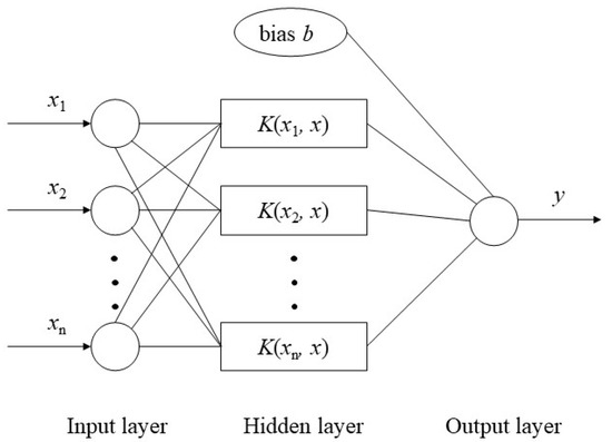
Figure 1.
Structure of support vector regression (SVR).
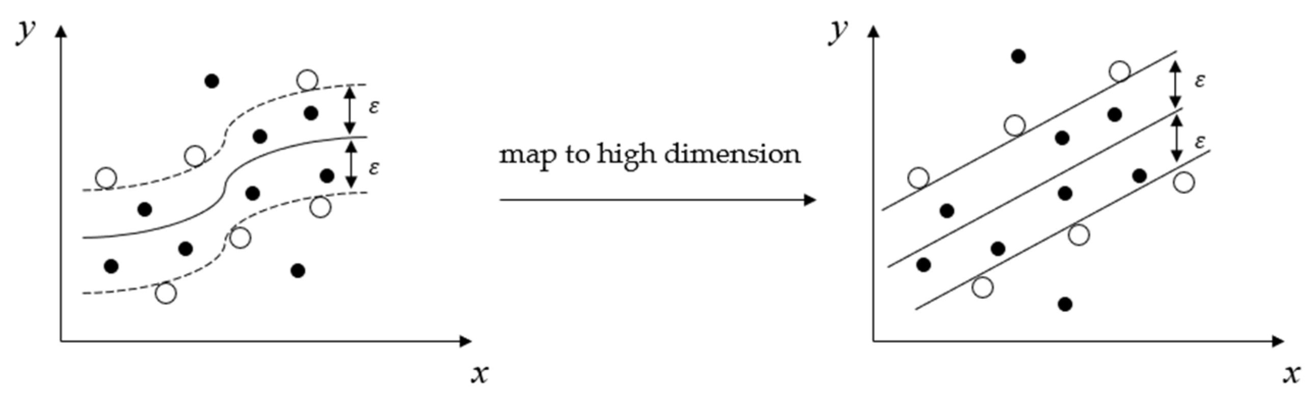
The basic principle of SVR is to map the feature vectors of sample data from low dimension to high dimension and perform regression analysis on them in high dimension by the usage of the kernel function, as shown in Figure 2. The function of the support vector regression machine is expressed as
where is the coefficient of the function; is the input feature vector; is the bias constant. To find the most value regression function, a minimization function needs to be established as follows:
where is the penalty factor, N is the number of samples; represents the predicted value of the feature vector of the number i sample; represents the true value of the feature vector of the number i sample; L is the linear insensitive loss function; is the maximum deviation.

Figure 2.
Schematic digamma of the kernel trick.
By establishing the Lagrange equation and the Karush–Kuhu–Tucker (KKT) condition to obtain the partial derivatives of the parameters [42], the dual-mode of the SVR model can be obtained. The final decision function is expressed as
where is the number of SVR machines; represents the optimal solution; is the kernel function in nonlinear regression, . A better kernel function is chosen, and the result is mapped to a high-dimensional space by calculating in a low-dimensional space, which effectively avoids the problem of dimensional explosion in a high-dimensional space.
References [43,44] reflect the applicability of the radial basis function (RBF) kernel in predicting nonlinear regression of engine response. Therefore, RBF was chosen in this paper; the RBF has high flexibility by adjusting kernel function coefficient , which can be shown as:
Above all, penalty factor C, kernel function coefficient , and the maximum deviation will all affect the result of SVR [43]. The parameters can be set in the efficient SVM regression learning toolbox LibSVM v3.4 [45], written by Professor Lin Chih-Jen.
2.3. The Model Training Process
In machine learning methods [46,47], normalization has widely been used to reduce the influence of the range of data. Therefore, in this research, a normalization method of (−1, 1) was chosen, which can be shown as
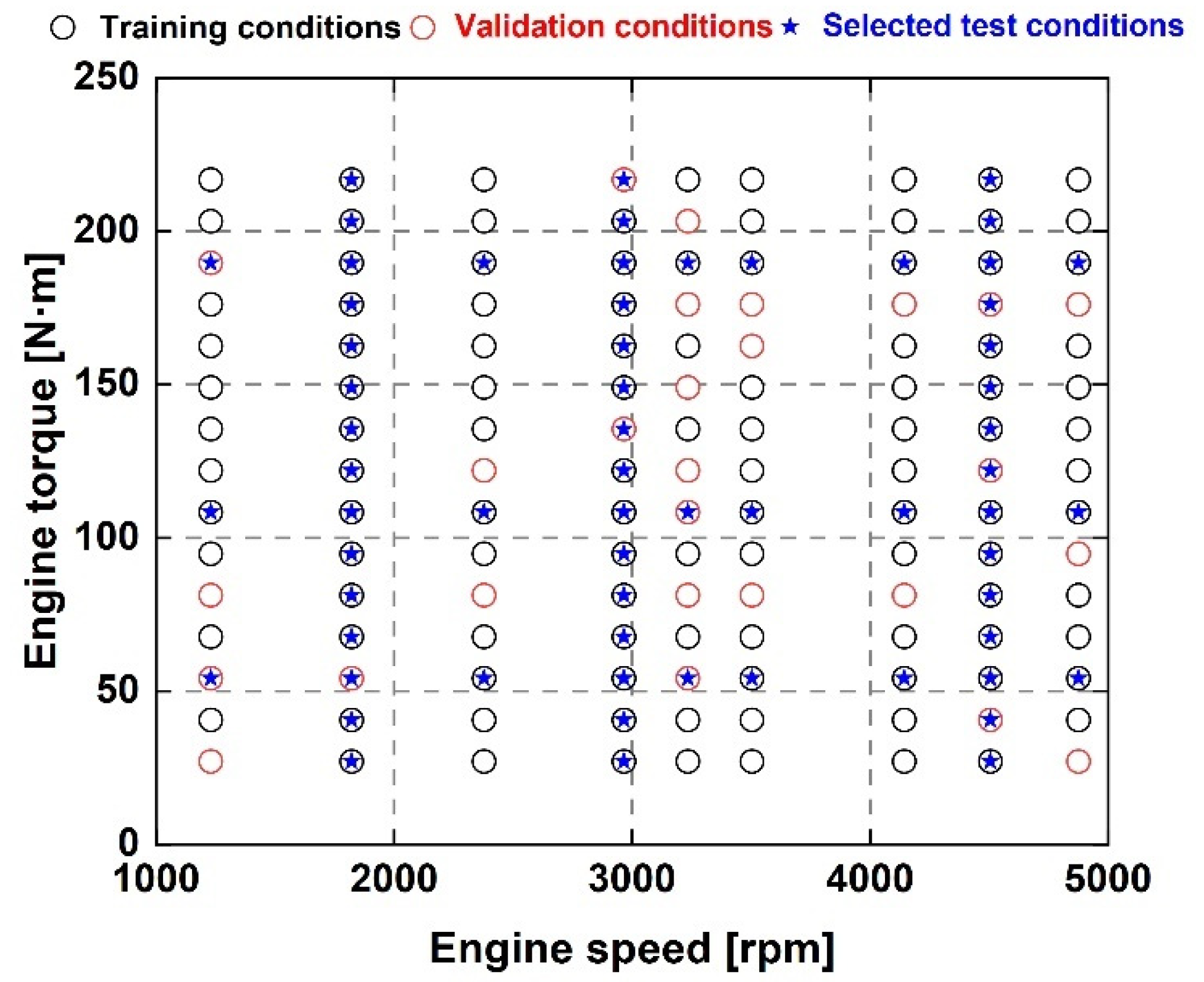
where x is the basic data, and y is the normalized data. After the results are obtained, it is necessary to operate inverse normalization. To evaluate the performance of the SVR method, the training and test datasets were randomly divided from 135 experimental data, as shown in Figure 3, and accounted for 80% and 20%, respectively. References [48,49] indicated that this percentage separation was recommended for the engine model in this research.
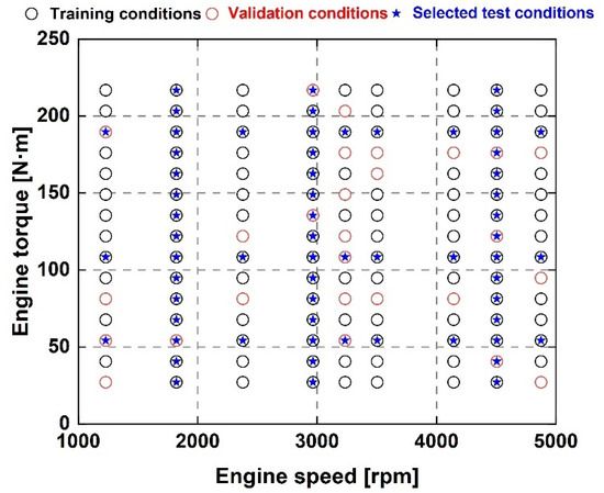
Figure 3.
Training, validation, and test data for machine learning approaches.
To further evaluate the success of the training model, steady-state datasets were utilized. As shown in Figure 3, 45 of 135 groups were selected, testing the prediction ability of the SVR model for engine performance under different engine loads with certain speeds (i.e., 1820, 2965, and 4505 RPM). Moreover, 27 of 135 groups were used to evaluate whether the engine speed effect on engine performance can be predicted by the prediction model under certain loads (i.e., 54, 108, and 188 N·m).
The statistical determination coefficient (R2) and root-mean-squared error (RMSE) can be used to evaluate the prediction performance. When R2 and RMSE are close to 1 and 0, respectively, it means the predicted value fits the measured value well, and the predictions are accurate. R2 and RMSE are defined as follows:
where is the predicted data; is the average value of the measured data; is the experimental data; n is the quantity of data.
The SVR model establishment process is shown in Figure 4. Firstly, preprocessing of data including loading and normalization was carried out, and then, appropriate hyperparameters of SVR were selected to make the RMSE as small as possible. Then, the prediction ability of the SVR model obtained by training was evaluated.
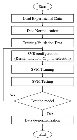
Figure 4.
Flowchart of SVR model [50].
3. Results and Discussion
This section discusses the precision of the SVR model predictions of the fuel consumption rate, NOx, CO, and HC emissions.
3.1. Discussion of Indicated Specific Fuel Consumption and Emissions Prediction
Figure 5, Figure 6, Figure 7 and Figure 8 show the comparison between the measured data and SVR predicted results. It is found that the majority of points were close to the diagonal line of slope = 1, suggesting a satisfactory prediction performance. Moreover, the hyperparameter sets are shown in the front of each figure. As the distribution of each data was different, the setting of hyperparameters was also different. Moreover, was selected as 0.01 for each indicator to improve the prediction accuracy [44].
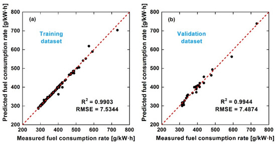
Figure 5.
Comparison of SVR predicted results with measured data of fuel consumption. (a) Training dataset; (b) Validation dataset.
Figure 5.
Comparison of SVR predicted results with measured data of fuel consumption. (a) Training dataset; (b) Validation dataset.
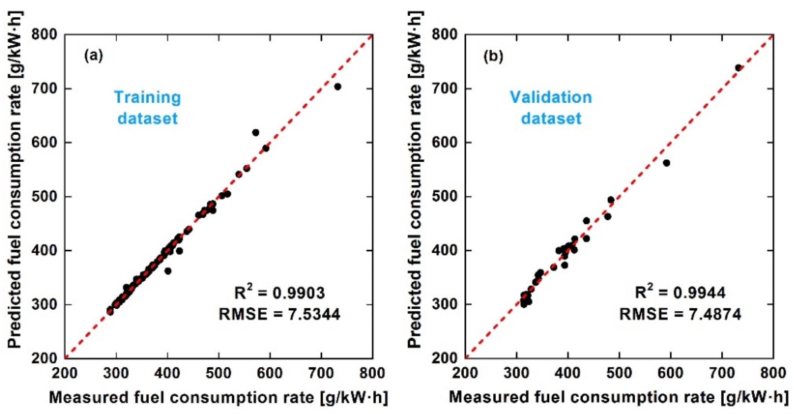
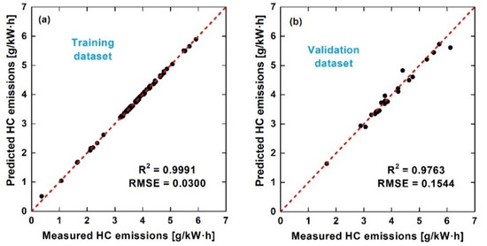
Figure 6.
Comparison of SVR predicted results with measured data of HC emissions. (a) Training dataset; (b) Validation dataset.
Figure 6.
Comparison of SVR predicted results with measured data of HC emissions. (a) Training dataset; (b) Validation dataset.
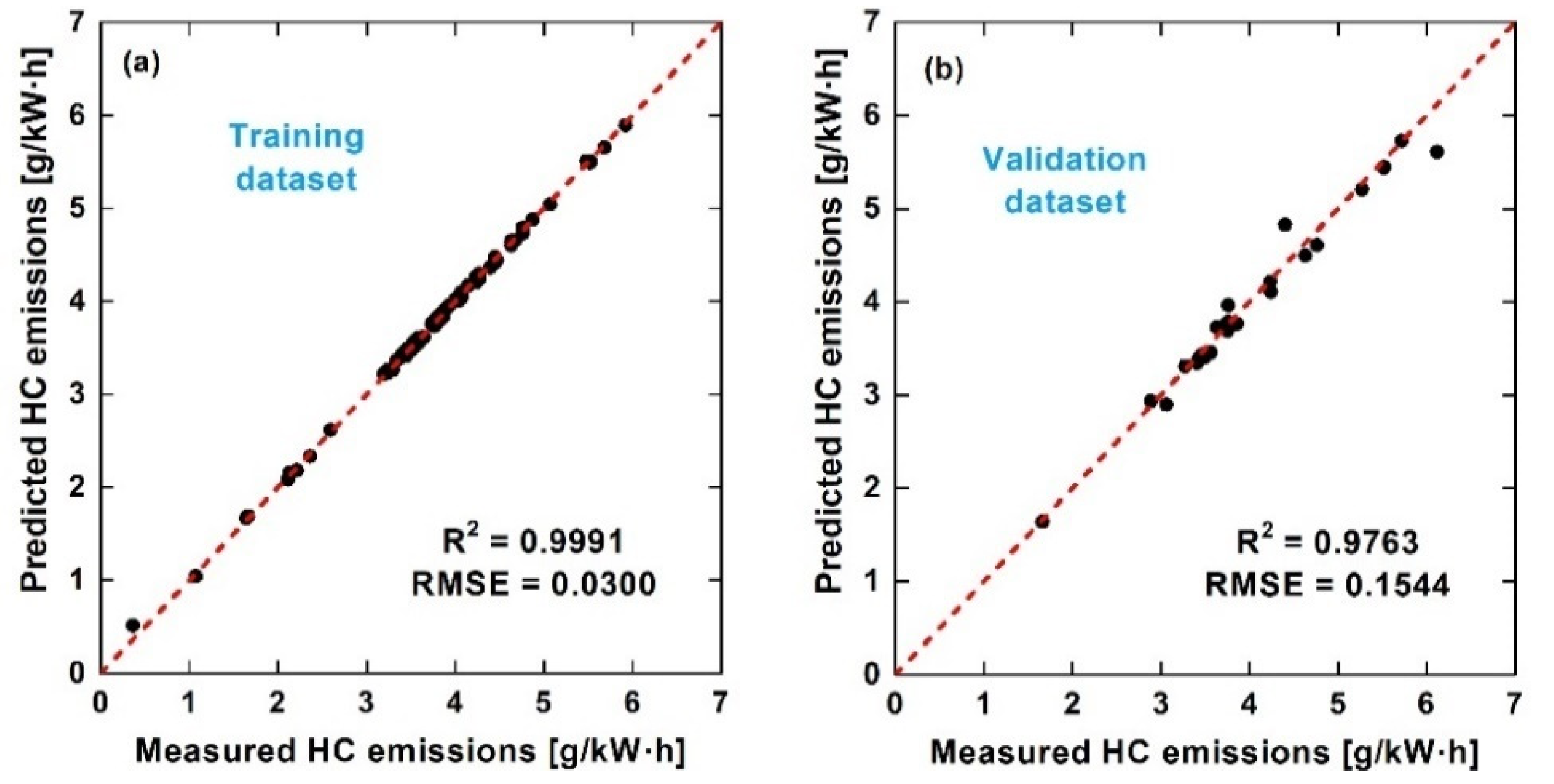

Figure 7.
Comparison of SVR predicted results with measured data of CO emissions. (a) Training dataset; (b) Validation dataset.
Figure 7.
Comparison of SVR predicted results with measured data of CO emissions. (a) Training dataset; (b) Validation dataset.
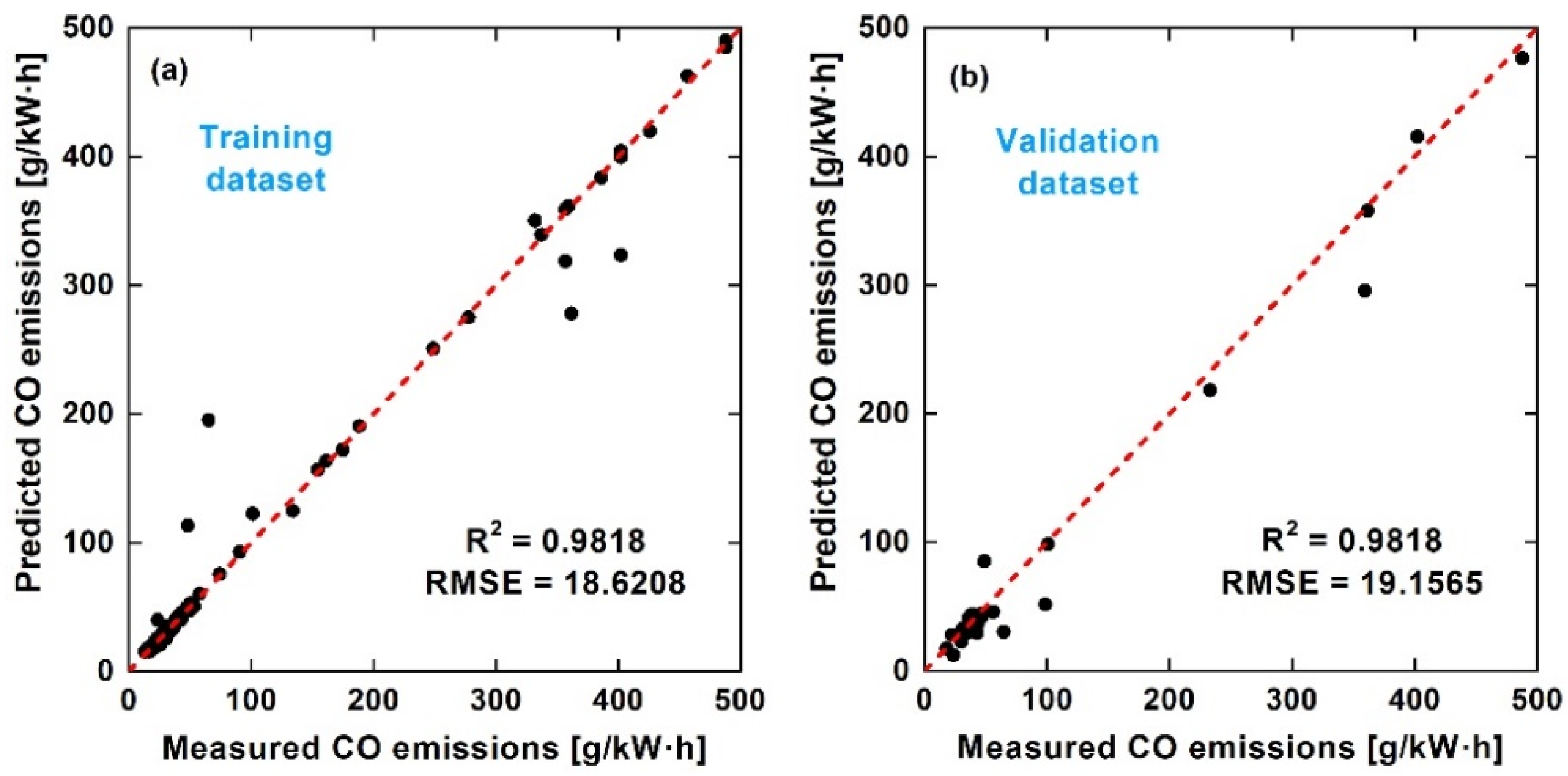

Figure 8.
Comparison of SVR predicted results with measured data of NOx emissions. (a) Training dataset; (b) Validation dataset.
Figure 8.
Comparison of SVR predicted results with measured data of NOx emissions. (a) Training dataset; (b) Validation dataset.
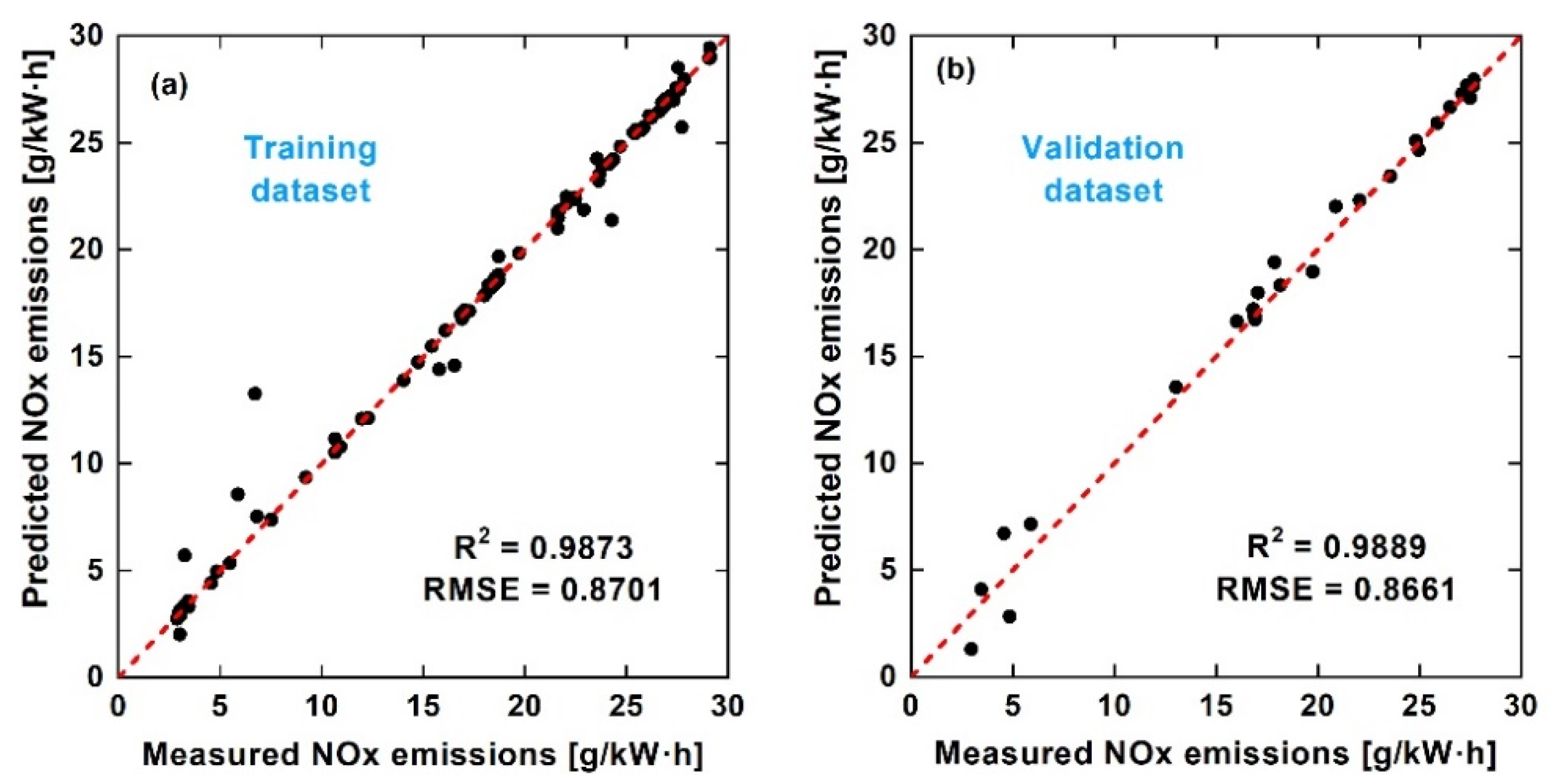
The R2 and RMSE of the fuel consumption for the training dataset were 0.9903, 7.5344, and for the validation dataset, these values were 0.9944 and 7.4874. The R2 and RMSE of the HC emissions training dataset were 0.9991, 0.03, and for the validation dataset, these values were 0.9818 and 0.1544. The R2 and RMSE of the CO emissions training dataset were 0.9818, 18.6208, and for the validation dataset, these values were 0.9818 and 19.1565. The R2 and RMSE of the NOx emissions training dataset were 0.9873, 0.8701, and for the validation dataset, they were 0.9889 and 0.8661. As shown in Figure 5, for the fuel consumption, the indicators of the validation dataset were both better than the training dataset, indicating the generalization ability of the SVR model. As shown in Figure 7, for the CO emissions prediction, very few points deviated far from the diagonal, caused by the possible overfitting, but the effect on R2 was very small. There is an order of magnitude difference in CO concentration between lean and rich combustion. Small changes in the equivalence ratio of the stoichiometry control would result in large changes in CO emission levels, making model predictions difficult [51].
The prediction results of the model were highly coincidental with the experimental data, which was also supported by the clustered points near the diagonal. The performance of the SVR training dataset and validation dataset were close, showing that the SVR model had good generalization ability in engine performance prediction. Generally, the R2 values were all near to 1, suggesting that the SVR model had successfully learned the relationship between engine inputs and outputs. Compared with Table 1, the R2 values in this paper were all higher than 0.95, indicating the high prediction precision for the SVR method. All these results showed that the SVR prediction model can predict the engine response under different engine speeds and loads conditions. When trained properly, the error was acceptable [36].
3.2. Discussion of Steady-State Prediction
In Section 3.1, the accuracy of SVR prediction for each performance indicator was illustrated by analyzing relevant statistical indicators (i.e., R2 and RMSE). In this section, a discussion is provided on whether the SVR model developed in this study can accurately describe the effect of input changes on output responses. In other words, it is crucial to investigate and monitor the ability to understand the complex relationships in machine learning training [44,52]. In order to obtain good engine emission performance and low fuel consumption, the electronic control unit of the gasoline engine changes the combustion condition in the cylinder by changing the throttle position and ignition advance timing of the engine, thus changing the load and speed. Due to the engine control strategy, a close relationship exists between engine input and response. Figure 9 and Figure 10 are used to evaluate whether the SVR model can predict the performance, emissions characteristics of the gasoline engine.
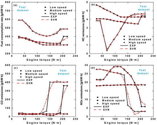
Figure 9.
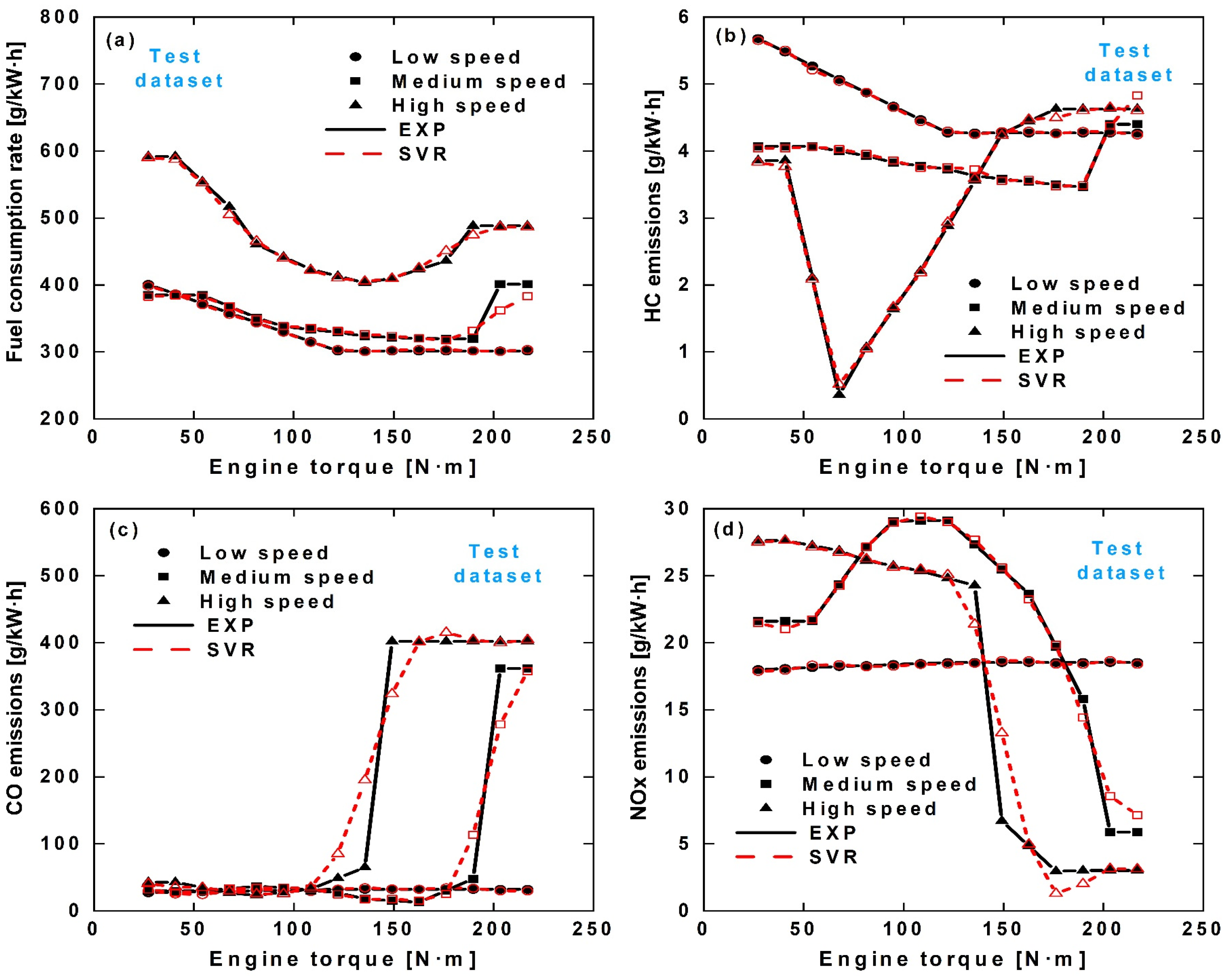
Comparison of SVR predicted data with experimentally measured under different engine torques. (a) Fuel consumption rate; (b) HC emissions; (c) CO emissions; (d) NOx emissions.

Figure 10.
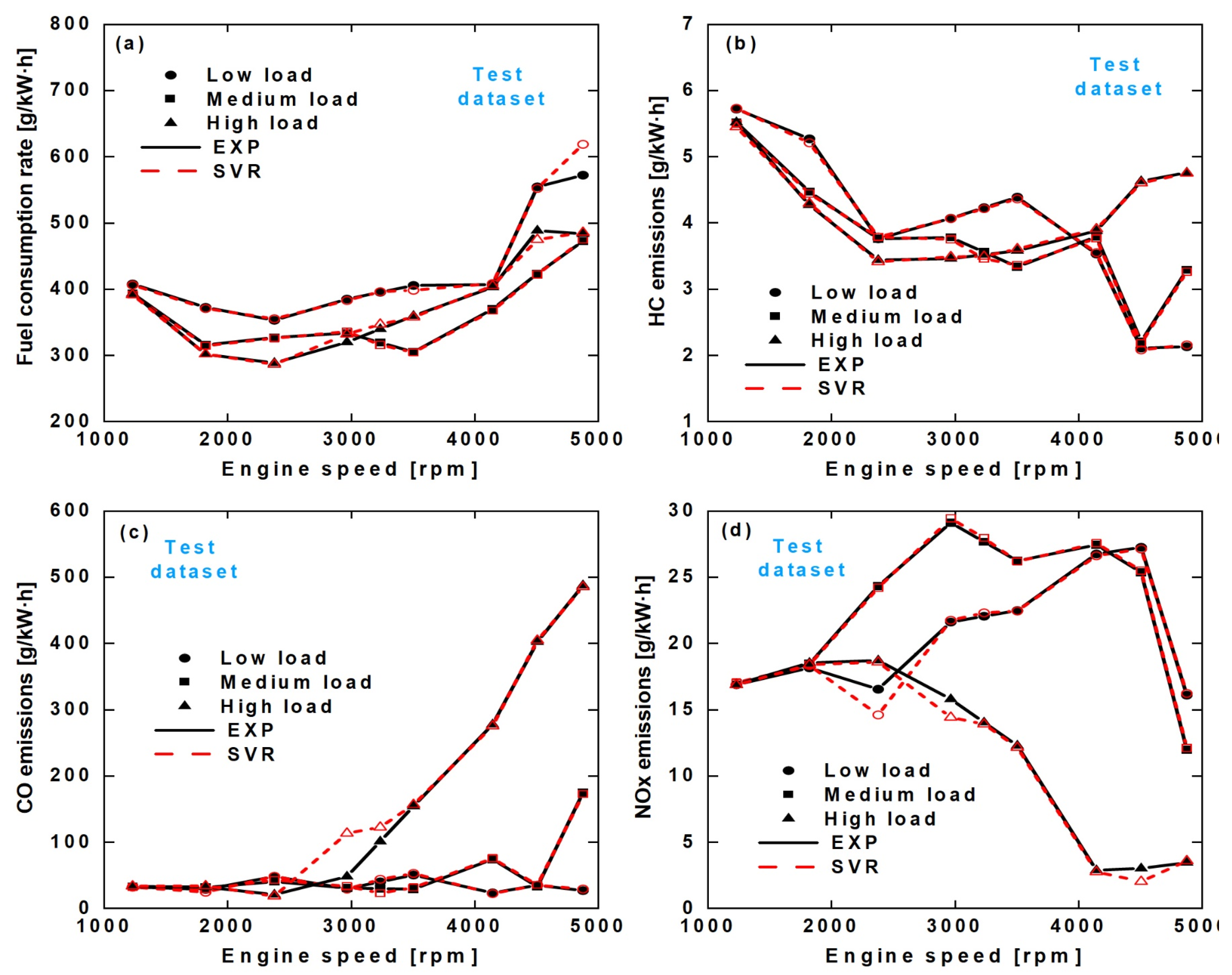
Comparison of SVR predicted data with experimentally measured under different engine speeds. (a) Fuel consumption rate; (b) HC emissions; (c) CO emissions; (d) NOx emissions.
Figure 9 shows the experimental and model prediction of the effects of torque on fuel consumption, HC, CO, and NOx emissions at 1820, 2965, and 4505 RPM speeds of the engine, respectively. Figure 9a shows the predicted fuel consumption, and it can be seen that, at medium and low speeds, the fuel consumption was close, while at high speed, a significant increase in fuel consumption was observed; as the load increased, the fuel consumption first decreased and then increased. This trend was similar to HC emissions, as shown in Figure 9b, indicating that a high-performance region existed that allows for better in-cylinder combustion and less emission generation. Figure 9c shows the prediction of CO emissions, a load value was found, and once the load exceeded this value, the CO emissions increased significantly. The turning point coincided with the point of increase in fuel consumption, indicating that, at higher loads, combustion efficiency of the engine decreased, and the incomplete products increased. Figure 9d shows the prediction of NOx emissions, which was less at low and medium load conditions, and more at high load conditions, indicating that the combustion deteriorated, the in-cylinder temperature reduced, and the NOx emissions generation decreased. Generally, the SVR model successfully reflected the influence of load on fuel consumption.
Figure 10 shows the impact of engine speed on fuel consumption and emissions under 54, 108, and 188 N·m engine loads, respectively. Figure 10a shows the prediction of fuel consumption rate, which is more sensitive to engine speed. Figure 10b presents the prediction of HC emissions, which decreased and then increased as the speed increased. In the most economical operating condition, it is less generated, which indicates high combustion efficiency. At higher speeds, the combustion efficiency of the engine decreased, and the amount of HC emissions increased, which was evident at high load, because of more fuel injected in the cylinder. Figure 10c shows the CO emission prediction, under high load conditions, due to less reaction time, more fuel injection volume, and uneven air–fuel mixture, the combustion was not sufficient and incomplete, which made the CO increase significantly. Figure 10d shows the NOx emissions prediction, at high speed; the NOx emissions generation was less due to insufficient combustion resulting in low in-cylinder temperature. As for the evaluation of the ML method prediction precisions, the SVR model captured the variation trend in these parameters under different speeds and could predict engine performance under different operating with small errors.
3.3. Discussion of Engine Performance Map Prediction
Based on Section 3.2, the prediction ability of the SVR model proved to be acceptable, and the ML model can describe the relationship between the engine input. To better investigate the applicability of SVR to performance prediction, the experimental values, predicted values, and errors of fuel consumption rate, HC, CO, and NOx emissions were obtained as different responses in Figure 11, Figure 12, Figure 13 and Figure 14, with the engine speeds and loads as independent variables.
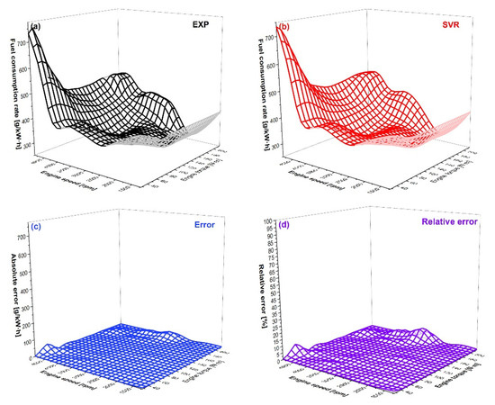
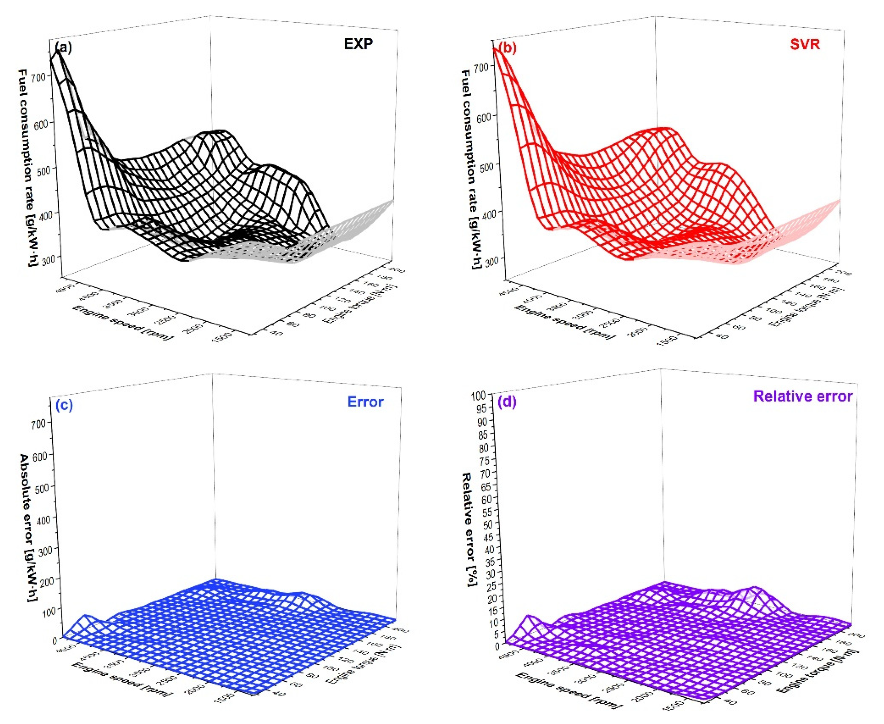
Figure 11.
Comparison of SVR-predicted and experimental fuel-consumption-rate-established engine map. (a) The experimental data; (b) The SVR-predicted data; (c) The absolute error; (d) The relative error.
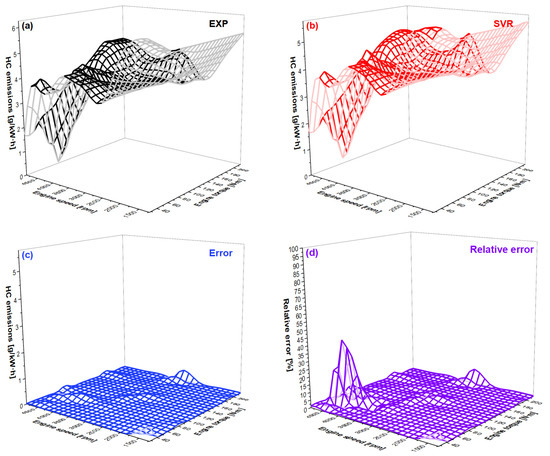
Figure 12.
Comparison of SVR-predicted and experimental HC-emissions-established engine map. (a) The experimental data; (b) The SVR-predicted data; (c) The absolute error; (d) The relative error.

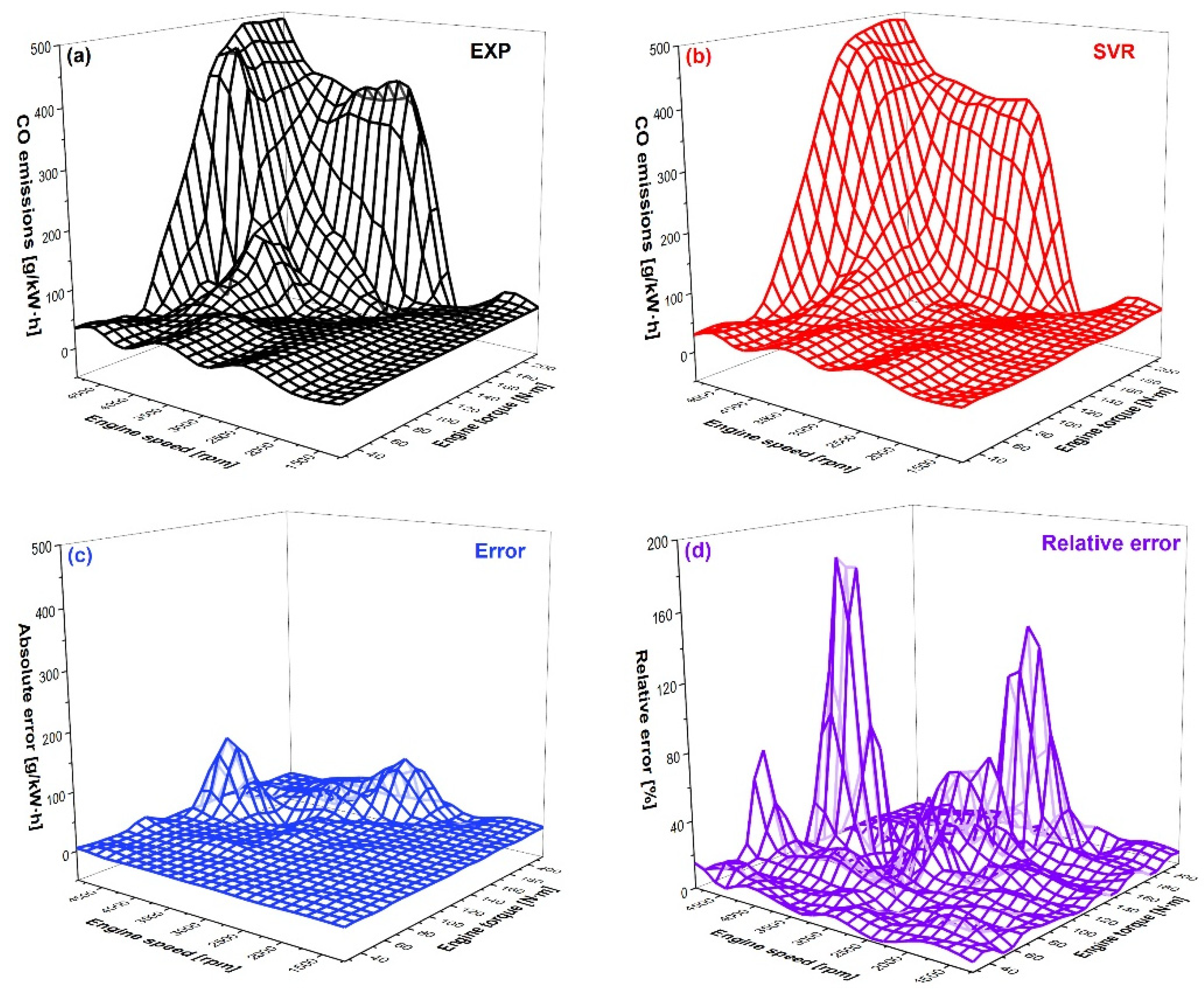
Figure 13.
Comparison of SVR-predicted and experimental CO-emissions-established engine map. (a) The experimental data; (b) The SVR-predicted data; (c) The absolute error; (d) The relative error.
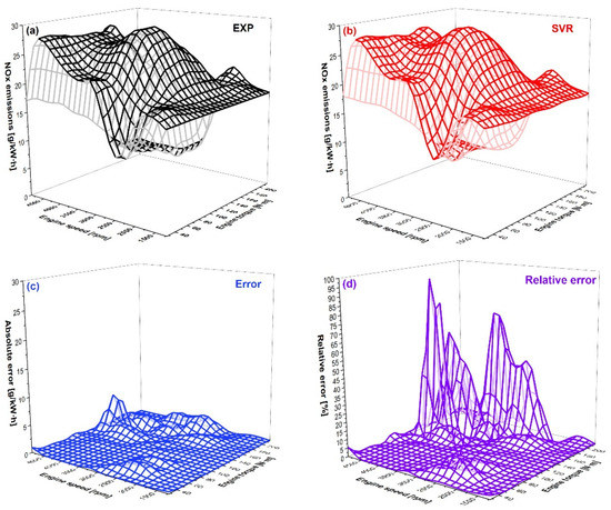
Figure 14.
Comparison of SVR-predicted and experimental NOx-emissions-established engine map. (a) The experimental data; (b) The SVR-predicted data; (c) The absolute error; (d) The relative error.
It can be seen in Figure 11 that, at lower loads and higher speeds, the fuel consumption rate increased, which was due to less power demanded but more fuel injection. As the load increased, the power required increased, and then, the fuel consumption was more adequate. As shown in Figure 12, HC emissions were generated less as engine speed increased [53], due to the faster air-fuel mixture flowing, the mixture uniformity was improved, and more HC was oxidized. CO emissions were generated more in high speed and high loading conditions, as shown in Figure 13, because the ECU (Electronic Control Unit) allowed the engine to work on a slightly oxygen-enriched mixture, converting CO into CO2. It can be seen in Figure 14 that NOx emissions were generated most at medium load and speed because the combustion was best at this condition, and the oxidation process was sufficient, caused by the high in-cylinder temperature. As shown in Figure 11c, Figure 12, Figure 13c and Figure 14c, the absolute prediction error of the SVR model for the results is small, which indicates that SVR can be used as a reference for setting conditions.
As for the relative error analyses, the relative error of fuel consumption rate prediction was the smallest. The errors of HC emissions were relatively large under high speed with low loading conditions, due to noise in the test data, leading to a decrease in the prediction accuracy of the ML method. The errors of CO and NOx emissions were larger under high speed with high loading conditions. NOx emissions were generated in a small amount (close to 0) under these working conditions, and the relative errors were relatively large. In comparison, the error in CO emissions might be due to the difficulty in controlling the equivalent ratio under these operations, which needed more engine power, and the sudden increase in injected oil made the data collected vary greatly.
4. Conclusions
The purpose of this paper was to assess the ability of SVR methods to predict the performance of the fuel consumption rate and emissions of a calibrated spark-ignition engine at the required engine speed and load. The results indicated that SVR algorithms can achieve this goal with acceptable errors. The main findings were as follows:
- (1)
- Our previous research found that artificial neural networks can help predict engine performance and emissions, at least for the gasoline engine discussed in this study. However, it required heavy tuning of the hyperparameters, such as the net structure. In contrast, the SVR algorithm employed in this study had a more convenient tuning process during the supervised learning process. Moreover, model performance regarding the training and validation datasets was improved. As a result, the SVR algorithm was suitable to be used for engine combustion-related parameters forecasting. In addition, the SVR model can help establish the engine mapping because the algorithm well correlated the engine control variables and engine responses, which can help reduce the effort during engine development.
- (2)
- As for the engine response prediction performance, fuel consumption rate and NOx emissions were predicted with good accuracy, while HC and CO emissions were predicted with a little less accuracy, compared with the first two. The underlying reason was the nature of the engine response. Specifically, HC emissions were unevenly distributed because HC concentration mainly depended on the trapped mass inside the crevice. With respect to CO emissions, variation in the equivalence ratio would dramatically change the CO concentration. This was because there is an order of magnitude difference in CO concentration between lean and rich combustion. Small changes in the equivalence ratio of the stoichiometry control would result in large changes in CO emission levels, making model predictions difficult. As a result, the combination of machine learning and carbon balance has the potential to further improve the performance of incomplete combustion production concentration predictions if carbon dioxide can be well forecasted, which will be the future direction of this study.
Author Contributions
Conceptualization, methodology, simulation, Y.Z.; validation, writing—original draft preparation, Q.W.; methodology, simulation, X.C.; writing—original draft preparation, Y.Y.; validation, R.Y.; analysis, supervision, Z.L.; validation, methodology, simulation, J.F. All authors have read and agreed to the published version of the manuscript.
Funding
This research was jointly funded by the 2021 “Teacher Professional Development Program” for domestic visiting scholars in universities (FX2021105).
Institutional Review Board Statement
Not applicable.
Informed Consent Statement
Not applicable.
Data Availability Statement
The data presented in this study are available on request from the corresponding author.
Acknowledgments
This study was jointly funded by the 2021 “Teacher Professional Development Program” for domestic visiting scholars in universities (FX2021105), which is gratefully acknowledged for providing the equipment and the right to use the software provided by Power Machinery and Vehicular Engineering Institute, Zhejiang University.
Conflicts of Interest
The authors declare no conflict of interest.
References
- Stocchi, I.; Liu, J.; Dumitrescu, C.E.; Battistoni, M.; Grimaldi, C.N. Effect of Piston Crevices on the Numerical Simulation of a Heavy-Duty Diesel Engine Retrofitted to Natural-Gas Spark-Ignition Operation. J. Energy Resour. Technol. 2019, 141, 112204. [Google Scholar] [CrossRef]
- Dumitrescu, C.E.; Padmanaban, V.; Liu, J. An Experimental Investigation of Early Flame Development in an Optical Spark Ignition Engine Fueled with Natural Gas. J. Eng. Gas Turbines Power. 2018, 140, 082802. [Google Scholar] [CrossRef]
- Bommisetty, H.; Liu, J.; Kooragayala, R.; Dumitrescu, C. Fuel Composition Effects in a CI Engine Converted to SI Natural Gas Operation (No. 2018-01-1137). SAE Tech. Pap. 2018, 1–8. [Google Scholar] [CrossRef] [Green Version]
- Huang, Q.; Bhattacharyya, D. Optimal Sensor Network Design for Multi-Scale, Time-Varying Differential Algebraic Equation Systems: Application to an Entrained-Flow Gasifier Refractory Brick. Comput. Chem. Eng. 2020, 141, 106985. [Google Scholar] [CrossRef]
- Schafer, F.; Schäfer, F.; Van Basshuysen, R. Reduced Emissions and Fuel Consumption in Automobile Engines; Springer Science and Business Media: Berlin/Heidelberg, Germany, 1995. [Google Scholar]
- Liu, J.; Ulishney, C.; Dumitrescu, C.E. Predicting the Combustion Phasing of a Natural Gas Spark Ignition Engine Using the K-Nearest Neighbors Algorithm. In Proceedings of the ASME International Mechanical Engineering Congress and Exposition, Virtual Conference, 16–19 November 2020. [Google Scholar] [CrossRef]
- Akgül, A. A Novel Method for a Fractional Derivative with Non-Local and Non-Singular Kernel. Chaos Solitons Fractals 2018, 114, 478–482. [Google Scholar] [CrossRef]
- Akgül, A.; Karatas Akgül, E. A Novel Method for Solutions of Fourth-Order Fractional Boundary Value Problems. Fractal Fract. 2019, 3, 33. [Google Scholar] [CrossRef] [Green Version]
- Akgül, E.K.; Akgül, A.; Yavuz, M. New Illustrative Applications of Integral Transforms to Financial Models with Different Fractional Derivatives. Chaos Solitons Fractals 2021, 146, 110877. [Google Scholar] [CrossRef]
- Akgül, A.; Akgül, E.K.; Baleanu, D.; Inc, M. New Numerical Method for Solving Tenth Order Boundary Value Problems. Mathematics 2018, 6, 245. [Google Scholar] [CrossRef] [Green Version]
- Kılıcman, A.; Khan, Y.; Akgul, A.; Faraz, N.; Akgul, E.K.; Inc, M. Analytic Approximate Solutions for Fluid Flow in the Presence of Heat and Mass Transfer. Therm. Sci. 2018, 22 (Suppl. 1), 259–264. [Google Scholar] [CrossRef] [Green Version]
- Heywood, J.B. Internal Combustion Engine Fundamentals; McGraw-Hill Education: Ney York, NY, USA, 2018. [Google Scholar]
- Liu, J.; Dumitrescu, C. CFD Simulation of Metal and Optical Configuration of a Heavy-Duty CI Engine Converted to SI Natural Gas. Part 2: In-Cylinder Flow and Emissions (No. 2019-01-0003). SAE Tech. Pap. 2019, 1–8. [Google Scholar] [CrossRef]
- Liu, J.; Dumitrescu, C. CFD Simulation of Metal and Optical Configuration of a Heavy-Duty CI Engine Converted to SI Natural Gas. Part 1: Combustion Behavior (No. 2019-01-0002). SAE Tech. Pap. 2019, 1–8. [Google Scholar] [CrossRef]
- Liu, Z.; Zuo, Q.; Wu, G.; Li, Y. An Artificial Neural Network Developed for Predicting of Performance and Emissions of a Spark ignition Engine Fueled with Butanol–Gasoline Blends. Adv. Mech. Eng. 2018, 10, 1687814017748438. [Google Scholar] [CrossRef]
- Ambrogi, L.; Liu, J.; Battistoni, M.; Dumitrescu, C.; Gasbarro, L. CFD Investigation of the Effects of Gas’ Methane Number on the Performance of a Heavy-Duty Natural-Gas Spark-Ignition Engine. SAE Tech. Pap. 2019. [Google Scholar] [CrossRef]
- Sui, W.; Hall, C.M. Combustion Phasing Modeling and Control for Compression Ignition Engines with High Dilution and Boost Levels. Proc. Inst. Mech. Eng. Part D J. Automob. Eng. 2018, 233, 1834–1850. [Google Scholar] [CrossRef] [Green Version]
- Liu, J.; Wang, H. Machine Learning Assisted Modeling of Mixing Timescale for LES/PDF of High-Karlovitz Turbulent Premixed Combustion. Combust. Flame 2022, 238, 111895. [Google Scholar] [CrossRef]
- Liu, J.; Ulishney, C.; Dumitrescu, C.E. Application of Random Forest Machine Learning Models to Forecast Combustion Profile Parameters of a Natural Gas Spark Ignition Engine. In Proceedings of the ASME International Mechanical Engineering Congress and Exposition, Virtual Conference, 16–19 November 2020. [Google Scholar] [CrossRef]
- Laubscher, R.; Rousseau, P. An Integrated Approach to Predict Scalar Fields of a Simulated Turbulent Jet Diffusion Flame Using Multiple Fully Connected Variational Autoencoders and MLP Networks. Appl. Soft Comput. 2021, 101, 107074. [Google Scholar] [CrossRef]
- Liu, J.; Ulishney, C.; Dumitrescu, C.E. Random Forest Machine Learning Model for Predicting Combustion Feedback Information of a Natural Gas Spark Ignition Engine. J. Energy Resour. Technol. 2021, 143, 012301. [Google Scholar] [CrossRef]
- Masikos, M.; Demestichas, K.; Adamopoulou, E.; Theologou, M. Energy-Efficient Routing Based on Vehicular Consumption Predictions of a Mesoscopic Learning Model. Appl. Soft Comput. 2015, 28, 114–124. [Google Scholar] [CrossRef]
- Deng, Y.; Zhu, M.; Xiang, D.; Cheng, X. An Analysis for Effect of Cetane Number on Exhaust Emissions from Engine with the Neural Network. Fuel 2002, 81, 1963–1970. [Google Scholar] [CrossRef]
- Liu, J.; Ulishney, C.; Dumitrescu, C.E. Comparative Performance of Machine Learning Algorithms in Predicting Nitrogen Oxides Emissions of a Heavy Duty Natural Gas Spark Ignition Engine. In Proceedings of the International Conference on Applied Energy, Bangkok, Thailand, 29 November–5 December 2020. [Google Scholar]
- Yusaf, T.F.; Buttsworth, D.; Saleh, K.H.; Yousif, B. CNG-Diesel Engine Performance and Exhaust Emission Analysis with the Aid of Artificial Neural Network. Appl. Energy 2010, 87, 1661–1669. [Google Scholar] [CrossRef]
- Liu, J.; Huang, Q.; Ulishney, C.; Dumitrescu, C.E. Prediction of Exhaust Gas Temperature of a Natural Gas Spark Ignition Engine Using Machine Learning Methods. In Proceedings of the International Conference on Applied Energy, Bangkok, Thaliand, 1–10 December 2020. [Google Scholar]
- Liu, J.; Huang, Q.; Ulishney, C.; Dumitrescu, C.E. Machine Learning Assisted Prediction of Exhaust Gas Temperature of a Heavy-Duty Natural Gas Spark Ignition Engine. Appl. Energy 2021, 300, 117413. [Google Scholar] [CrossRef]
- Parlak, A.; Islamoglu, Y.; Yasar, H.; Egrisogut, A. Application of Artificial Neural Network to Predict Specific Fuel Consumption and Exhaust Temperature for a Diesel Engine. Appl. Therm. Eng. 2006, 26, 824–828. [Google Scholar] [CrossRef]
- Liu, J.; Ulishney, C.; Dumitrescu, C.E. Improving Machine Learning Model Performance in Predicting the Indicated Mean Effective Pressure of a Natural Gas Engine. In Proceedings of the American Society of Mechanical Engineers Internal Combustion Engine Division Fall Technical Conference, Virtual Conference, 4–6 November 2020. [Google Scholar]
- Blurock, E.S.; Tuner, M.; Mauss, F. Phase Optimized Skeletal Mechanisms for Engine Simulations. Combust. Theory Model. 2010, 14, 295–313. [Google Scholar] [CrossRef]
- Chong, L.W.; Rengasamy, D.; Wong, Y.W.; Rajkumar, R.K. Load Prediction Using Support Vector Regression. In Proceedings of the IEEE International Joint Conference on Neural Networks, Penang, Malaysia, 5–8 November 2017; pp. 1069–1074. [Google Scholar] [CrossRef]
- Aliramezani, M.; Norouzi, A.; Koch, C.R. Support Vector Machine for a Diesel Engine Performance and NOx Emission Control-Oriented Model. IFAC—Pap. 2020, 53, 13976–13981. [Google Scholar] [CrossRef]
- Najafi, G.; Ghobadian, B.; Moosavian, A.; Yusaf, T.; Mamat, R.; Kettner, M.; Azmi, W.H. SVM and ANFIS for Prediction of Performance and Exhaust Emissions of a SI Engine with Gasoline–Ethanol Blended Fuels. Appl. Therm. Eng. 2016, 95, 186–203. [Google Scholar] [CrossRef] [Green Version]
- Liu, J.; Huang, Q.; Ulishney, C.; Dumitrescu, C. A Support-Vector Machine Model to Predict the Dynamic Performance of a Heavy-Duty Natural Gas Spark Ignition Engine. SAE Tech. Pap. 2021. [Google Scholar] [CrossRef]
- Rezaei, J.; Shahbakhti, M.; Bahri, B.; Aziz, A.A. Performance Prediction of HCCI Engines with Oxygenated Fuels Using Artificial Neural Networks. Appl. Energy 2015, 138, 460–473. [Google Scholar] [CrossRef]
- Niu, X.; Yang, C.; Wang, H.; Wang, Y. Investigation of ANN and SVM Based on Limited Samples for Performance and Emissions Prediction of a CRDI-Assisted Marine Diesel Engine. Appl. Therm. Eng. 2017, 111, 1353–1364. [Google Scholar] [CrossRef]
- Liu, J.; Ulishney, C.; Dumitrescu, C.E. Prediction of Efficient Operating Conditions Inside a Heavy-Duty Natural Gas Spark Ignition Engine Using Artificial Neural Networks. In Proceedings of the ASME 2020 International Mechanical Engineering Congress and Exposition, Virtual Conference, 16–19 November 2020. [Google Scholar] [CrossRef]
- Yang, R.; Yan, Y.; Sun, X.; Wang, Q.; Zhang, Y.; Fu, J.; Liu, Z. An Artificial Neural Network Model to Predict Efficiency and Emissions of a Gasoline Engine. Processes 2022, 10, 204. [Google Scholar] [CrossRef]
- Fu, J.; Yang, R.; Li, X.; Sun, X.; Li, Y.; Liu, Z.; Zhang, Y.; Sunden, B. Application of Artificial Neural Network to Forecast Engine Performance and Emissions of a Spark Ignition Engine. Appl. Therm. Eng. 2022, 201, 117749. [Google Scholar] [CrossRef]
- Mishra, C.; Subbarao, P. Design, Development and Testing a Hybrid Control Model for RCCI Engine Using Double Wiebe Function and Random Forest Machine Learning. Control Eng. Pract. 2021, 113, 104857. [Google Scholar] [CrossRef]
- Huang, Q.; Liu, J.; Ulishney, C.; Dumitrescu, C.E. On the Use of Artificial Neural Networks to Model the Performance and Emissions of a Heavy-Duty Natural Gas Spark Ignition Engine. Int. J. Engine Res. 2021, 14680874211034409. [Google Scholar] [CrossRef]
- Duan, H.; Huang, Y.; Mehra, R.K.; Song, P.; Ma, F. Study on Influencing Factors of Prediction Accuracy of Support Vector Machine (SVM) Model for NOx Emission of a Hydrogen Enriched Compressed Natural Gas Engine. Fuel 2018, 234, 954–964. [Google Scholar] [CrossRef]
- Gordon, D.; Norouzi, A.; Blomeyer, G.; Bedei, J.; Aliramezani, M.; Andert, J.; Koch, C.R. Support Vector Machine Based Emissions Modeling Using Particle Swarm Optimization for Homogeneous Charge Compression Ignition Engine. Int. J. Engine Res. 2021, 14680874211055546. [Google Scholar] [CrossRef]
- Wang, H.; Ji, C.; Shi, C.; Ge, Y.; Wang, S.; Yang, J. Development of Cyclic Variation Prediction Model of the Gasoline and N-Butanol Rotary Engines with Hydrogen Enrichment. Fuel 2021, 299, 120891. [Google Scholar] [CrossRef]
- Chang, C.-C.; Lin, C.-J. LIBSVM: A Library for Support Vector Machines. ACM Trans. Intell. Syst. Technol. 2011, 2, 1–27. [Google Scholar] [CrossRef]
- Liu, J.; Huang, Q.; Ulishney, C.; Dumitrescu, C.E. Comparison of Random Forest and Neural Network in Modelling the Performance and Emissions of a Natural Gas Spark Ignition Engine. J. Energy Resour. Technol. 2022, 144, 032310. [Google Scholar] [CrossRef]
- Liu, J.; Ulishney, C.; Dumitrescu, C.E. Machine Learning Assisted Analysis of Heat Transfer Characteristics of a Heavy Duty Natural Gas Engine (No. 2022-01-0473). SAE Tech. Pap 2022, 1–8. [Google Scholar] [CrossRef]
- Shahpouri, S.; Norouzi, A.; Hayduk, C.; Rezaei, R.; Shahbakhti, M.; Koch, C.R. Hybrid Machine Learning Approaches and a Systematic Model Selection Process for Predicting Soot Emissions in Compression Ignition Engines. Energies 2021, 14, 7865. [Google Scholar] [CrossRef]
- Hao, D.; Mehra, R.K.; Luo, S.; Nie, Z.; Ren, X.; Fanhua, M. Experimental Study of Hydrogen Enriched Compressed Natural Gas (HCNG) Engine and Application of Support Vector Machine (SVM) on Prediction of Engine Performance at Specific Condition. Int. J. Hydrogen Energy 2019, 45, 5309–5325. [Google Scholar] [CrossRef]
- Ahmad Yasmin, N.S.; Abdul Wahab, N.; Ismail, F.S.; Musa, M.A.; Halim, M.H.; Anuar, A.N. Support Vector Regression Modelling of an Aerobic Granular Sludge in Sequential Batch Reactor. Membranes 2021, 11, 554. [Google Scholar] [CrossRef] [PubMed]
- Gasbarro, L.; Liu, J.; Dumitrescu, C.; Ulishney, C.; Battistoni, M.; Ambrogi, L. Heavy-Duty Compression-Ignition Engines Retrofitted to Spark-Ignition Operation Fueled with Natural Gas. SAE Tech. Pap. 2019, 74, 1–31. [Google Scholar]
- Ji, C.; Wang, H.; Shi, C.; Wang, S.; Yang, J. Multi-Objective Optimization of Operating Parameters for a Gasoline Wankel Rotary Engine by Hydrogen Enrichment. Energy Convers. Manag. 2020, 229, 113732. [Google Scholar] [CrossRef]
- Huang, Z.; Miao, H.; Zhou, L.; Jiang, D. Technical Note: Combustion Characteristics and Hydrocarbon Emissions of a Spark Ignition Engine Fuelled with Gasoline-Oxygenate Blends. Proc. Inst. Mech. Eng. Part D J. Automob. Eng. 2000, 214, 341–346. [Google Scholar] [CrossRef]


Publisher’s Note: MDPI stays neutral with regard to jurisdictional claims in published maps and institutional affiliations. |
© 2022 by the authors. Licensee MDPI, Basel, Switzerland. This article is an open access article distributed under the terms and conditions of the Creative Commons Attribution (CC BY) license (https://creativecommons.org/licenses/by/4.0/).