A Population Balance Methodology Incorporating Semi-Mechanistic Residence Time Metrics for Twin Screw Granulation

Abstract

This work is concerned with the incorporation of semi-mechanistic residence time metrics into population balance equations for twin screw granulation processes to predict key properties. From the historical residence time and particle size data sourced, process parameters and equipment configuration information were fed into the system of equations where the input flow rates and model compartmentalization varied upon the parameters. Semi-mechanistic relations for the residence time metrics were employed to predict the particle velocities and dispersion coefficients in the axial flow direction of the twin screw granulation. The developed model was then calibrated for several experimental run points in each data-set. The predictions were evaluated quantitatively through the parity plots. The root mean square error (RMSE) was used as a metric to compare the degree of goodness of fit for different data-sets using the developed semi-mechanistic relations. In summary, this paper presents a more mechanistic but simplified approach of feeding residence time metrics into the population balance equations for twin screw granulation processes.

1. Introduction

1.1. Twin Screw Granulation Population Balance Development

Systems of population balance equations (PBEs) have been the most popular approach for modeling granulation processes, both batch and continuous because of change in particle size distributions due to processing conditions. In a system model described by PBEs, particles are grouped according to their key attributes such as size, liquid content, porosity, and spatial positions. One of the key tenets of employing PBEs to solve a process model is that all particles with same internal attributes and external positions will behave similarly. PBEs are formulated as first-order partial integro-differential equations with respect to both time and spatial locations in the system, and the rate of growth and death of each particle class is a function of the number of particles currently available of the said class and other classes such as those forming the particles.

The generic expression of a PBE is as follows in Equation (1):

$$\begin{array}{cc}\hfill & \frac{\partial N\left(x,y,z,s,l,g,t\right)}{\partial t}+\frac{\partial }{\partial x}\left(N\left(x,y,z,s,l,g,t\right)\frac{\partial x}{\partial t}\right) + \frac{\partial }{\partial y}\left(N\left(x,y,z,s,l,g,t\right)\frac{\partial y}{\partial t}\right)\hfill \\ \hfill & +\frac{\partial }{\partial z}\left(N\left(x,y,z,s,l,g,t\right)\frac{\partial z}{\partial t}\right) + \frac{\partial }{\partial s}\left(N\left(x,y,z,s,l,g,t\right)\frac{\partial s}{\partial t}\right)\hfill \\ \hfill & + \frac{\partial }{\partial l}\left(N\left(x,y,z,s,l,g,t\right)\frac{\partial l}{\partial t}\right) + \frac{\partial }{\partial g}\left(N\left(x,y,z,s,l,g,t\right)\frac{\partial g}{\partial t}\right)\hfill \\ \hfill & ={\Re }_{Aggregation}\left(x,y,z,s,l,g,t\right) + {\Re }_{Breakage}\left(x,y,z,s,l,g,t\right) + {\Re }_{Nucleation}\left(x,y,z,s,l,g,t\right)\hfill \\ \hfill & + F{\left(x,y,z,s,l,g,t\right)}_{In}-F{\left(x,y,z,s,l,g,t\right)}_{Out}\hfill \end{array}$$

(1)

where $N\left(x,y,z,s,l,g,t\right)$ is the number of particles, $\left(x,y,z\right)$ are the positional co-ordinates, $\left(s,l,g\right)$ are the solid, liquid and gas content of the particles, t is the time co-ordinate, $\Re {\left(x,y,z,s,l,g,t\right)}_{Aggregation}$ is the net rate of change of particles due to aggregation, $\Re {\left(x,y,z,s,l,g,t\right)}_{Breakage}$ is the net rate of change of particles due to breakage and $\Re {\left(x,y,z,s,l,g,t\right)}_{Nucleation}$ is the net rate of change of particles due to nucleation mechanism, $F{\left(x,y,z,s,l,g,t\right)}_{In}$ is the number of particles flowing in and $F{\left(x,y,z,s,l,g,t\right)}_{Out}$ is the number of particles flowing out. For a continuous wet granulation system, the terms on the left-hand side of the equation represents the rate of change with respect to time, the spatial positions in the granulator, solid content, moisture content, and gas porosity in the granules. There are several empirical parameters in the rate expressions. Different theories and models variations express differently these rates processes, with the ultimate objective of achieving fully mechanistic representation of the rate processes.

PBE models have been extensively developed and are still being researched and updated in order to completely and accurately characterize continuous wet granulation processes [1,2].

Ramachandran and Chaudhury [3] developed a model to design and control a continuous drum granulation process. The study presented a compartmentalized PBE for a pilot-plant scale simulation. The simulation results showed that that the average diameter, moisture content, and bulk density of the outlet granules could be controlled by manipulating the nozzle spray rates of the liquid binder and the feed rates of the inflow solid powder blends. A model was developed to control the particle size distributions of the granules, with binder distribution on the powder particles in the granulator as a new manipulated variable.

Barrasso et al. [4] presented a continuous PBE model that simulated the difference in PSDs and composition for a two-component system (API and excipient), liquid binder content, and the porosity of granules. The results showed good agreement with experimental trends. In Barrasso et al.’s subsequent work [5], a calibrated and validated PBE model was developed where the empirical rate constants and parameters were determined using experimental data.

Kumar et al. [6] presented a 1D PBE model that included aggregation and breakage processes for a twin-screw granulation (TSG) process. The model parameters and their respective 95% confidence range were estimated using experimentally measured PSDs. The model was accordingly used for predicting granulation outcomes within the design space of the experiments. Moreover, operating conditions were identified, where the different granulation mechanism regimes could be separated in distinct compartments in the granulator, which would enable one to control each mechanism accordingly and influence the granule size distribution as needed.

Shirazian et al. [7] in their work presented a regime-separated model where, in addition to modeling, the conveying and kneading elements as different types of ideal liquid reactors, the relative mechanism rates, aggregation, and breakage were varied for different zones. The conveying element zones were assumed to favor granule formation through aggregation and the kneading elements were assumed to be conducive towards breakage of granules. McGuire et al. [8,9] also are one of the few researchers to have incorporate residence time distribution (RTD) into PBEs by assuming an average mean residence time (MRT) which translated into a constant axial velocity of the particles at all locations for all attributes.

Hauwermeiren et al. [10] also developed a compartmental PBE for TSG system where different mechanism rate expressions were formulated for the different locations of kneading zones based on whether the particles were being wetted due to liquid binder addition or not. Wang et al. [11] also contributed to the field of PBE development further by developing a breakage rate for particles that incorporated the equipment screw geometry.

It has been inferred from Positron Emission Particle Tracking (PEPT) studies [12] that kneading zones’ material holdup is more than that of the conveying screws. Therefore, the local MRT in the PBE has been assumed to be higher for kneading and lower for conveying sections accordingly. A discrete element method (DEM) study has also shown that average particle speeds decrease for increasing sizes [13]. However, the same study also showed that the particle velocities in the axial direction of transport decreased with size. The local variance is again dependent on the compartment’s mixing dynamics, and as seen in [14], sections having plug-flow behavior have zero axial dispersion and variance in RTD. On the other hand, sections behaving like pure mixing tanks have infinite dispersion and the normalized variances of the RTDs are equal to unity.

A few studies have focused on coupling discrete element method simulations to PBE models where the compartmental residence time information from DEM is fed to the PBE models [15,16]. However, the particles in the DEM simulations are scaled up, and wet granulation of particles is mimicked by cohesive mixing. Most importantly, DEMs are computationally expensive which makes it unfeasible to run them in tandem with PBE models for the full process length.

1.2. Objectives

From the above text, it can be inferred that the initial work in PBE development for TSG focused on developing the granulation rate mechanisms. However, little foray has been made into the development of expressions for axial flow/of particles. The flow is dictated by axial velocities and dispersions of the particles which can be calculated by from the semi-mechanistic MRT and variance models developed previously in Muddu et al. [17]. Therefore, the work described in this paper proposes to have a more granular expression for the axial velocities of particles that would be influenced by both the mean residence time (MRT) and variance of RTD, whereby the velocities will depend on size, liquid composition, and location inside the TSG equipment.

The rest of the paper is organized as described in this paragraph. Section 2 introduces two experimental datasets used in the study that have been sourced from existing published data in literature. Section 3 is concerned with the theoretical background of the paper and introduces the relations for the PBEs developed for the TSG systems studied along with the incorporation of previously developed semi-mechanistic relations for estimating MRT and variance of the system. Section 4 shows the results of the study and discusses the model prediction performance for different datasets. Section 5 is a short conclusion that summarizes the paper and provides suggestions for future researchers to improve and build upon the modeling scheme presented in this work.

2. Materials and Methods

The size (3 sieve fractions) and residence time metrics’ (MRT and variance) experimental data were collected from published available literature [18,19]. The data-set collated has been described below in

Table 1. Summary of the twin screw granulation RTD and sieve fractions available and collected from literature.

Data Source	Equipment Name	Process Material	Varied Parameters	Number of Data Points
Kumar et al., 2015 [18]	ConsiGma-25	$\alpha$-Lactose MH	FR, RPM, NK & SA	66
Kumar et al., 2016 [19]	ConsiGma-25	$\alpha$-Lactose MH	FR, RPM, LS, NK & SA	51
				Total: 117

. The data-set has been classified based on source, equipment dimensions, and varied process and equipment variables: powder feed rate (FR), processing screw speed (RPM), liquid-to-solid percentage (LS), screw configuration described by the number of kneading elements (NK), and stagger angle (SA) between them. The table also lists the available number of points sourced from each study.

In addition to the above-mentioned categories, the database also contained details on the extruder shaft outer diameter. and the true densities of the powder processing material and distilled water. The collation and categorization along these parameters aided us in building a modular PBE which can account for varying experimental run parameters.

3. Theory and Calculations

3.1. Particle Grid Configuration

As the granular bed contains solid formulation particles in varying proportions, the particles have been defined on the basis of their solid volume contents, which is a key coordinate to describing a particle’s dimensions and physical properties such as size, density, and porosity. Since the size of the particles has been defined and tracked by the available solid volume content s, the available liquid volume content l in each different class or ‘bin’ of particles has been tracked in a separate grid vector following the lumped parameter approach. The solid content has been varied independently in a geometric progression, and the initial amount of liquid in the feed powders has been kept to be zero. The ratio of the progression has been kept at $1.5$. As there is a large difference in the tracer particle size, primary lactose powder size and the final granule sieve cuts, 16 different classes of particles in the model were selected, whereby each size has been defined by the respective solid volume content. Therefore, the grid of particles is a one-dimensional (1D) grid and the resulting population balance model developed is also a 1D PBM with lumped liquid. The tracer particles have also been accounted for separately in a parallel grid with their own lumped liquid content. The reason for this approach is that the tracer particles would have their own flow and granulation properties such as axial velocity, dispersion coefficient, and agglomeration rate constants.

3.2. PBE Configuration

The material balance in the twin screw granulator (TSG) has been modeled in terms of population balance equations (PBEs), which track the change in particle size over time for different classes. PBEs are the established framework for particulate systems with distinct and evolving particle size distributions (PSDs). Moreover, PBEs are nearly indispensable where the rate processes depend on the particle sizes and compositions.

Therefore, a semi-mechanistic PBE model has been developed in which the equations were developed from the first principles, but some experimental data and/or material properties were used as input parameters to the rate equations.

The granulation process took into account the rate processes of the following phenomena: aggregation of the smaller particles into larger granules, breakage of larger particles into smaller particles, liquid addition due to distilled water spraying, bulk convective movement of material due to axial velocity, and diffusive flux of particles due to axial dispersion.

The PBE framework built to simulate and investigate the effects of RTD has been simplified to a monocomponent equation varying spatially only in the axial direction. Particle aggregation, breakage, and liquid addition mechanisms have been considered. The liquid content associated with each particle has been calculated separately as a lumped parameter in a parallel set of equations.

The PBE framework for TSG containing expressions for effects of the RTD can be described below in (2) and (3) as:

$$\begin{array}{cc}\hfill & \frac{\partial N\left(z,s,t\right)}{\partial t}+\frac{\partial }{\partial z}\left(v_{bulk}\left(z\right) \times N\left(z,s,t\right)\right)-\frac{{\partial }^2}{\partial z^2}\left(D_{bulk}\left(z\right) \times N\left(z,s,t\right)\right)\hfill \\ \hfill & =\Re {\left(z,s,t\right)}_{Agg}+\Re {\left(z,s,t\right)}_{Break}+\dot{F}{\left(z,s,t\right)}_{In}-\dot{F}{\left(z,s,t\right)}_{Out}\hfill \end{array}$$

(2)

$$\begin{array}{cc}\hfill & \frac{\partial }{\partial t}\left(N\left(z,s,t\right) \times l_{bulk}\left(z,s,t\right)\right)+\frac{\partial }{\partial z}\left(v_{bulk}\left(z\right) \times N\left(z,s,t\right)\times l_{bulk}\left(z,s,t\right)\right)\hfill \\ \hfill & -\frac{{\partial }^2}{\partial z^2}\left(D_{bulk}\left(z\right) \times N\left(z,s,t\right) \times l_{bulk}\left(z,s,t\right)\right)\hfill \\ \hfill & =\Re {\left(z,s,t\right)}_{Agg,Liq}+\Re {\left(z,s,t\right)}_{Break,Liq}+{\dot{L}}_{addn,bulk}\left(z,s,t\right)\hfill \\ \hfill & + \left(\dot{F}{\left(z,s,t\right)}_{In} \times l\left(z,s,t\right)\right)-\left(\dot{F}{\left(z,s,t\right)}_{Out} \times l\left(z,s,t\right)\right)\hfill \end{array}$$

(3)

where $N\left(z,s,t\right)$ is the number of bulk particles in axial position z and particle solid volume s at time t. $\Re {\left(z,s,t\right)}_{Agg}$ and $\Re {\left(z,s,t\right)}_{Break}$ are the net rates of bulk particles due to aggregation and breakage mechanisms, respectively, and $\Re {\left(z,s,t\right)}_{Agg,Liq}$ and $\Re {\left(z,s,t\right)}_{Break,Liq}$ are the net rates of change of liquid associated with bulk particles due to aggregation and breakage mechanisms, respectively. $\dot{F}{\left(z,s,t\right)}_{In}$ and $\dot{F}{\left(z,s,t\right)}_{Out}$ are the flow rates of particles coming in and out at axial location z. $l_{bulk}(z,s,t)$ is the associated liquid volume in bulk particle of solid volume s at location z and time t. ${\dot{L}}_{addn,particle}\left(z,s,t\right)$ is the rate of particulate liquid volume. Here, $v_{bulk}\left(z\right)$ and $D_{bulk}\left(z\right)$ are the convective velocity and axial dispersion coefficient of the particles in location z, respectively.

The equations for the tracer particles have been given analogously in (4) and (5) as:

$$\begin{array}{cc}\hfill & \frac{\partial M\left(z,s,t\right)}{\partial t} + \frac{\partial }{\partial z}\left(v_{tracer}\left(z\right) \times M\left(z,s,t\right)\right)-\frac{{\partial }^2}{\partial z^2}\left(D_{tracer}\left(z\right) \times M\left(z,s,t\right)\right)\hfill \\ \hfill & =\dot{G}{\left(z,s,t\right)}_{In}-\dot{G}{\left(z,s,t\right)}_{Out}\hfill \end{array}$$

(4)

$$\begin{array}{cc}\hfill & \frac{\partial }{\partial t}\left(M\left(z,s,t\right) \times l_{tracer}\left(z,s,t\right)\right) + \frac{\partial }{\partial z}\left(v_{tracer}\left(z\right) \times M\left(z,s,t\right) \times l_{tracer}\left(z,s,t\right)\right)\hfill \\ \hfill & -\frac{{\partial }^2}{\partial z^2}\left(D_{tracer}\left(z\right) \times M\left(z,s,t\right) \times l_{tracer}\left(z,s,t\right)\right)\hfill \\ \hfill & ={\dot{L}}_{addn,tracer}\left(z,s,t\right) + \left(\dot{G}{\left(z,s,t\right)}_{In} \times l_{tracer}\left(z,s,t\right)\right)-\left(\dot{G}{\left(z,s,t\right)}_{Out} \times l_{tracer}\left(z,s,t\right)\right)\hfill \end{array}$$

(5)

where $M\left(z,s,t\right)$ is the number of bulk particles in axial position z, and particle solid volume s at time t. $\dot{G}{\left(z,s,t\right)}_{In}$ and $\dot{G}{\left(z,s,t\right)}_{Out}$ are the flow rates of particles coming in and out at axial location z. $l_{tracer}(z,s,t)$ is the associated liquid volume in tracer particle of solid volume s at location z and time t. Here, $v_{tracer}\left(z\right)$ and $D_{tracer}\left(z\right)$ are the convective velocity and axial dispersion coefficient of the particles in location z, respectively.

It must be noted that, as the tracer particles were the API theophylline and the bulk powder bed consisted of just lactose without any binder particles, it has been assumed that the tracer would not agglomerate and get bounded either to themselves or the bulk particles.

The net aggregation rate for a general particle of bin class $\left(s\right)$ at time t is defined as follows:

$${\Re }_{Agg}(z,s,t)={\Re }_{Agg}^{form}(z,s,t)-{\Re }_{Agg}^{dep}(z,s,t),$$

(6)

where ${\Re }_{Agg}(z,s,t)$ is the net aggregation rate of any particular particle class at location z, ${\Re }_{Agg}^{form}(z,s,t)$ is the rate of formation of a particle due to aggregation during a binary collision of particles, and ${\Re }_{Agg}^{dep}(z,s,t)$ is the rate of depletion of particles due to collision with other particles.

The rate of formation of a particle of class $(z,s)$ due to aggregation of two smaller particles at a given time instant t is given similar treatment as a kinetic reaction and thus has been defined as follows:

$${\Re }_{Agg}^{form}(z,s,t) = \frac{1}{2}\sum _{s^{\prime }=s_{min}}^{s^{\prime }<s}\beta (z,s^{\prime },s-s^{\prime },t)N(z,s^{\prime },t)N(z,s-s^{\prime },t)$$

(7)

where is $s_{min}$ is the respective minimum solid volume for a particle, and $\beta (z,s^{\prime },s-s^{\prime }t)$ indicates the specific aggregation rate of any two particles whose net respective solid bin volumes equate to $\left(s\right)$ at location z.

The above equation takes into account all the possible ordered pair combinations such that the net volume of the colliding particles is equal to the volume of the particle whose formation rate is being tracked. The product of the aggregation kernel and the number of particles of each colliding ordered pair is multiplied by half as each possible combination is counted twice while performing the ordered pair multiplication.

The rate of depletion of a particle due to aggregation of the particle with another at a given time instant t is given as follows:

$${\Re }_{Agg}^{dep}(z,s,t)=N(z,s,t)\sum _{s^{\prime }=s_{min}}^s\beta (z,s^{\prime },s,t)N(z,s^{\prime },t)$$

(8)

It can be seen from (7) that the aggregation of particles is overall a second order process, and is directly proportional to the number/quantity of each colliding particle bin/ size class in the ordered pair.

The net breakage rate for a general particle of bin class $\left(s\right)$ at time t is defined as follows:

$${\Re }_{Brk}(z,s,t)={\Re }_{Brk}^{form}(z,s,t)-{\Re }_{Brk}^{dep}(z,s,t),$$

(9)

where ${\Re }_{Brk}(z,s,t)$ is the net breakage rate of any particular particle class at location z, ${\Re }_{Brk}^{form}(z,s,t)$ is the rate of formation of a particle due to breakage of particles, and ${\Re }_{Brk}^{dep}(z,s,t)$ is the rate of depletion of particles due to breakage.

The rate of formation of a particle of class $(z,s)$ due to breakage of a larger particle into two smaller particles at a given time instant t is expressed as:

$${\Re }_{Brk}^{form}(z,s,t)=\sum _{s^{\prime }>s}^{s_{max}}b(s,s^{\prime })K_{break}(z,s^{\prime },t)N(z,s^{\prime },t)$$

(10)

where is $s_{max}$ is the respective maximum volume of the solid particle, $b(s,s^{\prime })$ is the probability of a larger particle of volume $s^{\prime }$ breaking into s and $s^{\prime }-s$ at location z, and $K_{break}(z,s^{\prime },t)$ indicates the specific breakage rate of a particle whose net respective solid bin volumes equate to $\left(s\right)$ at location z. For the purpose of this study, it has been assumed that the larger particle has an equal chance to break into all the possible smaller sizes considered in the grid. Therefore, it can be formulated as $b(s,s^{\prime })=\frac{1}{z_{s^{\prime }}}$, where $z_{s^{\prime }}$ is the grid location of the larger particle undergoing breakage.

The rate of depletion of a particle of class $(z,s)$ due to breakage at a given time instant t is given as:

$${\Re }_{Brk}^{dep}(z,s,t)=K_{break}(z,s,t)N(z,s,t)$$

(11)

3.3. Aggregation and Breakage Rates

The aggregation rate kernel is akin to a kinetic reaction rate constant. However, in the PBM model developed in our study, the kernel rather depends on the properties of the colliding particles/granules. The kernel that was developed in [20] has been adapted in this work and described as follows:

$$\begin{array}{cc}\hfill & \beta (z,s^{\prime },s-s^{\prime },t)={\beta }_0((vol(z,s^{\prime },t) + vol(z,s-s^{\prime },t))\hfill \\ \hfill & \times \left(\right(\frac{100}{2}{\left(\frac{l_{bulk}(z,s^{\prime },t)}{vol(z,s^{\prime },t)} + \frac{l_{bulk}(z,s-s^{\prime },t)}{vol(z,s-s^{\prime },t)}\right)}^{\alpha }\hfill \\ \hfill & \times {\left(100-\frac{100}{2}\left(\frac{l_{bulk}(z,s^{\prime },t)}{vol(z,s^{\prime },t)} + \frac{l_{bulk}(z,s-s^{\prime },t)}{vol(z,s-s^{\prime },t)}\right)\right)}^{\delta }{)}^{\alpha }\hfill \end{array}$$

(12)

where $vol(z,s,t)$ is the total volume of the particle at time t and location z, and ${\beta }_0$, $\alpha$, and $\delta$ are empirical tuning constants. $\alpha$ is a liquid dependency enhancing parameter where the increasing liquid quantity per particle increases the granulation rate, and $\delta$ is a liquid dependency diminishing parameter where the increasing liquid quantity per particle caps the granulation rate.

The breakage rate is dependent on the particle size and the shear given to the particles. The expression that was developed in [21] has been adapted in this work and described as follows:

$$\begin{array}{c}\hfill K_{break}(z,s,t)=\frac{1}{2}{P}_1{G}_{shear}\left({\left(vol(z,s,t)\right)}^{P_2}\right)\end{array}$$

(13)

The expression for the shear rate is given as follows:

$$\begin{array}{c}\hfill G_{shear}=2\pi \left(RPM\right)\end{array}$$

(14)

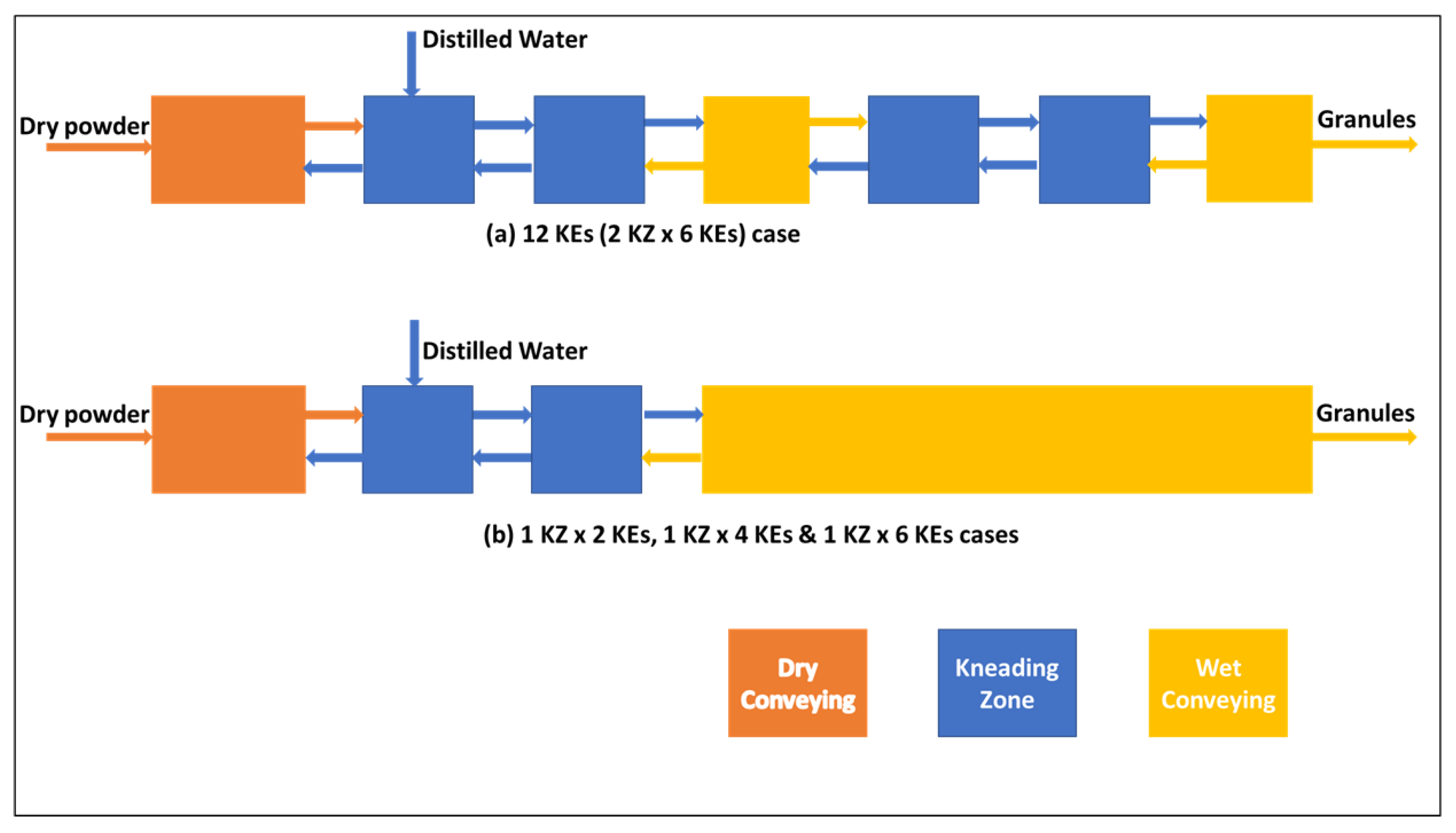
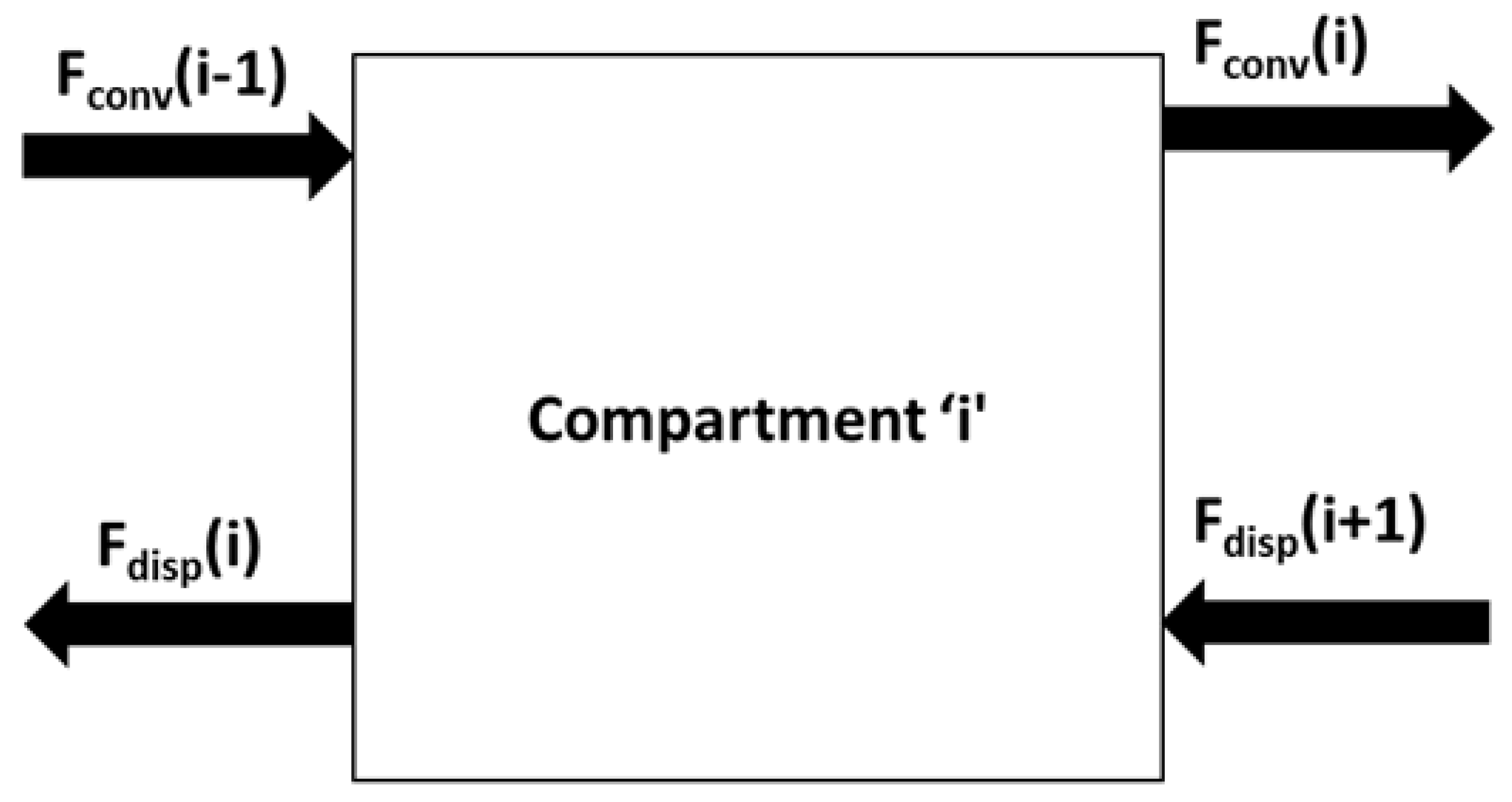
3.4. PBE Compartmentalization

As mentioned in Section 1, the mixing behavior in twin screw granulation equipment depends on the internal configurations. Screw conveying and kneading sections are the two main types of elements used in several TSG configurations. For the purpose of this study, each continuous section of screw elements was modeled as a single compartment, and each kneading section was modeled as two compartments. From Figure 1, it can be seen that all the granulation design of experiment (DOE) scenarios with twelve (12) NK (two (2) compartments of six (6) NK separated by a conveying section in each screw shaft) were modeled with seven (7) compartments. The remaining run cases with only a single kneading zone in the screw configuration were modeled as four (4) compartments.

Every compartment has been assumed to have both convective flow forward into the subsequent compartment and dispersive flow into the preceding compartment. This methodology was developed based on the ideas expressed in the works of Portillo et al. and Sen et al. [22,23]. This methodology has been pictorially shown below in Figure 2:

The convective flux from a compartment into the subsequent one has been formulated as:

$$F_{conv}\left(i\right)=\frac{v\left(i\right) \times N\left(i\right)}{L\left(i\right)}$$

(15)

where $L\left(i\right)$ is the length of the compartment i.

The dispersive flux has been similarly expressed as the flow of particles from a compartment into the preceding one, and it has been formulated as follows:

$$F_{disp}\left(i\right)=\frac{4 \times D\left(i\right) \times N\left(i\right)}{{\left(L\left(i\right)\right)}^2}$$

(16)

where $L\left(i\right)$ is the length of the compartment i.

3.5. Axial Velocities and Dispersion Coefficients

Every compartment had its own MRT and Péclet number calculated individually using the following relations:

$$MRT\left(z\right)=b_1\left(z\right) \times \frac{F{R}_{vol,net}^{b_2} \times Availvo{l}_{total}}{F{R}_{vol,net}^{b_3} \times Dispvolrat{e}_{conv,1lead}^{b_4}}$$

(17)

$$Pe\left(z\right)=b_5\left(z\right) \times \frac{F{R}_{vol,net}^{b_3} \times Dispvolrat{e}_{conv,1lead}^{b_4}}{\frac{S{A}_{knead,deg} \times Dispvolrat{e}_{conv,1lead}^{b_6} \times \pi }{N{K}_{knead}\times 180}}$$

(18)

with the constants subject to the following constraints:

$$-b_2 + b_3 + b_4=1$$

(19)

$$b_3 + b_4=b_6$$

(20)

The above equations have been explained in detail in [17], and will be briefly touched again here. The readers are encouraged to read our prior work to get a full flavor of the idea presented here. The term $F{R}_{vol,net}$ standing for the total volumetric flow rate of material into the compartment is either just that of the fed powder flow rate for the dry conveying section, or the net sum of the powder and liquid flow rate for the kneading and wet conveying sections. $Availvo{l}_{total}$ is the total available volume for the particles to occupy for the particular compartment, $Dispvolrat{e}_{conv,1lead}$ is the volume of material dispensed by one turn of the screws of the equipment, $S{A}_{knead,deg}$ is the stagger angle of the kneading elements in the compartmental section, and $N{K}_{knead}$ is the number of kneading elements per shaft in the compartmental section.

The MRT for each compartment has been formulated as pre-constant $b_1\left(z\right)$ multiplied by a holdup factor (numerator) divided by a flow factor (denominator). This was to mimic the chemical engineering definition of MRT while developing for particulate systems. The Péclet number for each compartment has been formulated as pre-constant $b{\left(z\right)}_5$ multiplied by a flow factor (numerator) divided by a mixing factor (denominator). This was again to mimic the chemical engineering definition of Péclet number (convection flow -to- dispersive flow). The terms described in previous paragraph have been raised to the corresponding exponents, which are in turn subject to the constraints described in (19) and (20) so that the predicted value of MRT is in time units (seconds) and that of the Péclet number is unitless (ratio).

As the MRT and Pe were evaluated individually for each compartment, the fitting constants, especially the pre-constants $b_1\left(z\right)$ and $b{\left(z\right)}_5$ were also different for every compartment. As there were three (3) different kinds of compartments: dry conveying, kneading, and wet conveying, $b_1\left(z\right)$ and $b{\left(z\right)}_5$ were separately estimated for each kind.

The estimated MRT for each compartment is the fed into the PBE model as the axial velocity of the bulk particles as follows:

$$v{\left(z\right)}_{bulk}=\frac{L\left(z\right)}{MRT\left(z\right)}$$

(21)

and the axial dispersion of the bulk particles is given by:

$$D{\left(z\right)}_{bulk}=\frac{{\left(L\left(z\right)\right)}^2}{MRT\left(z\right) \times Pe\left(z\right)}$$

(22)

The estimated axial velocity and axial dispersion coefficient of the tracer particles have been expressed relative to that of the respective values for the bulk particles as follows:

$$v{\left(z\right)}_{tracer}=\frac{v{\left(z\right)}_{bulk}}{MR{T}_{tracer}^{*}}$$

(23)

and the axial dispersion of the bulk particles is given by:

$$v{\left(z\right)}_{tracer}=\frac{D{\left(z\right)}_{bulk}}{MR{T}_{tracer}^{*} \times P{e}_{tracer}^{*}}$$

(24)

where $MR{T}_{tracer}^{*}$ is a dimensionless scaling constant indicating how greater or larger the residence time of the tracer is relative to the bulk material, and $P{e}_{tracer}^{*}$ is a dimensionless scaling constant indicating how greater or larger the mixing behavior of the tracer is relative to the bulk material.

3.6. Numerical Techniques

As mentioned in Section 3.1, the grid of particle sizes used for developing the PBE model is exponential in nature. Therefore, the number of particles was allocated in the appropriate grid locations, and the cell average technique as developed in [1] was employed where lever rule techniques are used to distribute particles in nearest grid locations by linear interpolations.

The system of differential Equations (1)–(5) were discretized using Euler’s first order finite forward difference method where the value of the unknown property at a subsequent time-step is given by the value at the present time-step, the rate expression governing the property and the time-step chosen.

An issue that arises while numerically solving the coupled differential equations over the process time is the value of the time-step chosen for the simulations. An adaptive time-step method was chosen where the time-step or interval of discretization is computed according to the Courant–Fredrichs–Lewis (CFL) condition.

3.7. Output Metrics

The PBE models were first run to steady state for each experimental run and the exiting granules were classified into three classes according to size: fines (<150 $\mathsf{\mu }$m), bulk (150–1000 $\mathsf{\mu }$m), and coarse (>1000 $\mathsf{\mu }$m). Once the steady state was reached at about 150 s of process simulation time, pulse tracer was added into the system, and the outlet concentration of tracer was computed. From the time profile of the tracer concentration, the MRT and the normalized variance of the in silico tracer experiment were computed.

3.8. Parameter Estimation

As PBE model simulations take quite some time, it becomes unfeasible to perform traditional parametric estimations by selecting at least 50% of the data points as the training set. Instead, for the purpose of this study, a few select runs were chosen (about 16–18 for each dataset) to train the model parameters such that the varying process parameters covered the range of the DOE of the datasets. The in-built fmincon function in MATLAB was used to arrive at the estimated parameter values based on initial guesses. The endpoint of the training was determined based on the weighted sum of the sum of square of errors (SSE) of the MRT, normalized variance, and the three (3) sieve fractions.

The general expression for SSE is given as:

$$SSE=\sum _{i=1}^n{\left(y_{i,exp}-y_{i,pred}\right)}^2$$

(25)

where $y_{i,exp}$ are the actual experimental values for the metric reported and $y_{i,pred}$ are the predicted values of the metric from the model.

The total weighted SSE expression was defined as follows:

$$SS{E}_{net}=1.2SS{E}_{MRT} + 0.8SS{E}_{Var} + 1.2SS{E}_{Bulk} + 0.9SS{E}_{Fines} + 0.9SS{E}_{Coarse}$$

(26)

From the expression, it is seen that the MRT contributed relatively greater to the SSE than the normalised variance, and the bulk size fraction also contributed greater than the fines and coarse size fractions.

Satisfactory parity plots, with realistic narrow upper and lower bounds set, were used as tools to evaluate the model’s performance on the datasets. The performance was determined based on how many predicted points fell between these limits, and, in addition, the root mean square of errors ($RMSE$) was also evaluated as a statistical measure for goodness of fit.

The expression is given as follows:

$$RMSE=\sqrt{\frac{{\displaystyle \sum _{i=1}^n}{\left(y_{i,exp}-y_{i,pred}\right)}^2}{n}}$$

(27)

where $y_{i,exp}$ are the actual experimental values for the metric reported and $y_{i,pred}$ are the predicted values of the metric from the model.

4. Results and Discussion

As mentioned previously in Section 3.8, 18 runs were chosen from the Kumar et al., 2015 dataset, and 16 runs were chosen from the Kumar et al., 2016 dataset for training the PBE model to the available residence time and particle size data, and consequently arrive at the optimal parameters for the aggregation kernel constants, breakage rate constants, residence time metrics constants, and tracer velocities and dispersion coefficients scaling constants. The values of the various constants and parameters used in the integrated model have been given below in

Table 2. The values of various model parameters estimated.

Constant	Kumar et al., 2015 [18] Value	Kumar et al., 2016 [19] Value	Unit
${\beta }_0$	9.38	7.91	×0.1 s${}^{-1}$
$\alpha$	0.13	0.10	-
$\delta$	0	0	-
$P_1$	38.77	80.86	-
$P_2$	0.28	0.24	-
$b_{1,dry}$	1.20	0.97	-
$b_{1,knead}$	0.16	0.15	-
$b_{1,wet}$	0.88	0.81	-
$b_{5,dry}$	7.19	1.13	-
$b_{5,knead}$	6.53	0.38	-
$b_{5,wet}$	5.18	1.14	-
$MR{T}_{tracer}^{*}$	0.55	0.45	-
$P{e}_{tracer}^{*}$	2.10	0.95	-

.

Here, it should be noted that $\delta$ value of 0 indicates that there is no diminishing effect of the increasing liquid quantity on the granulation rate.

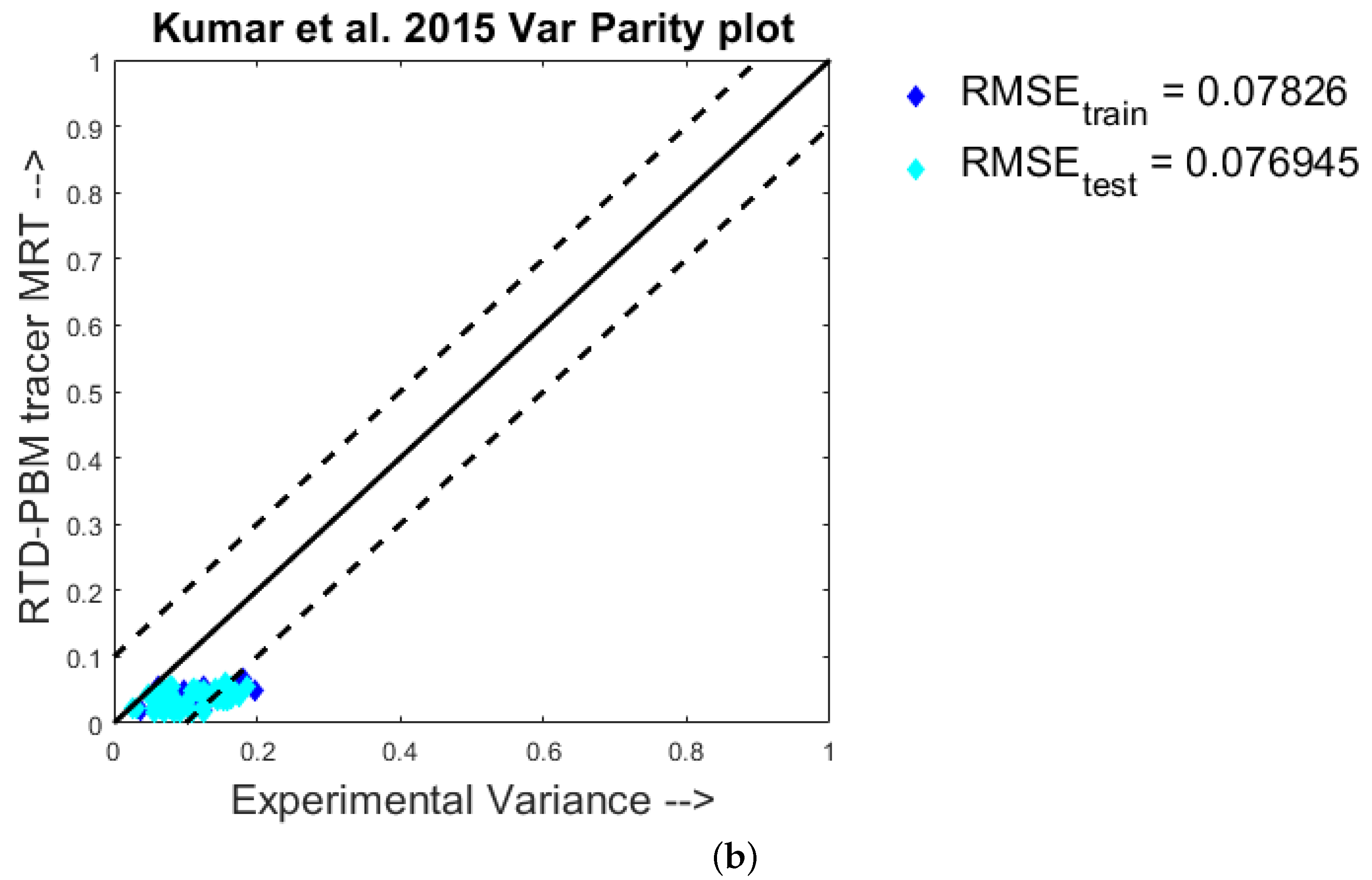
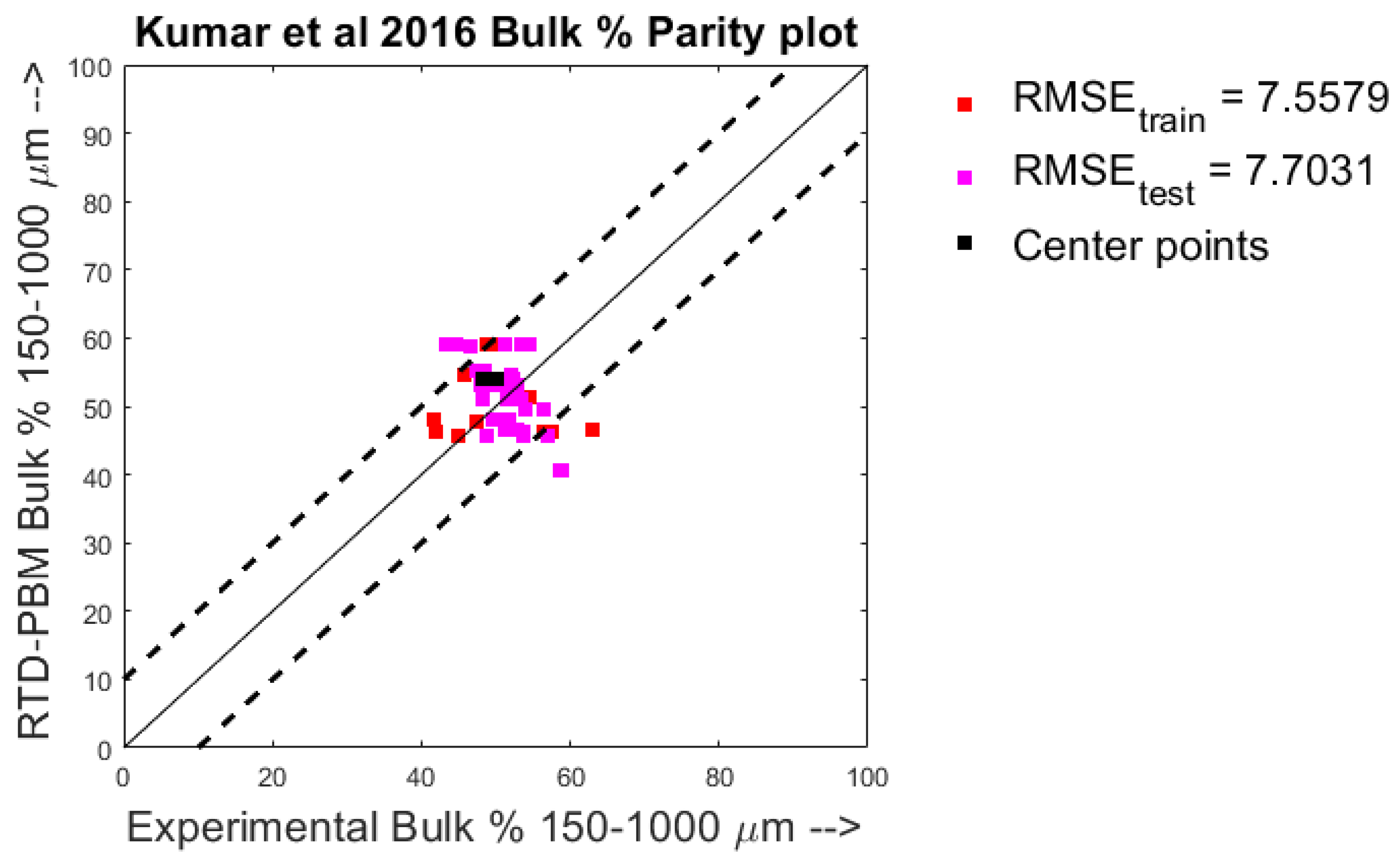
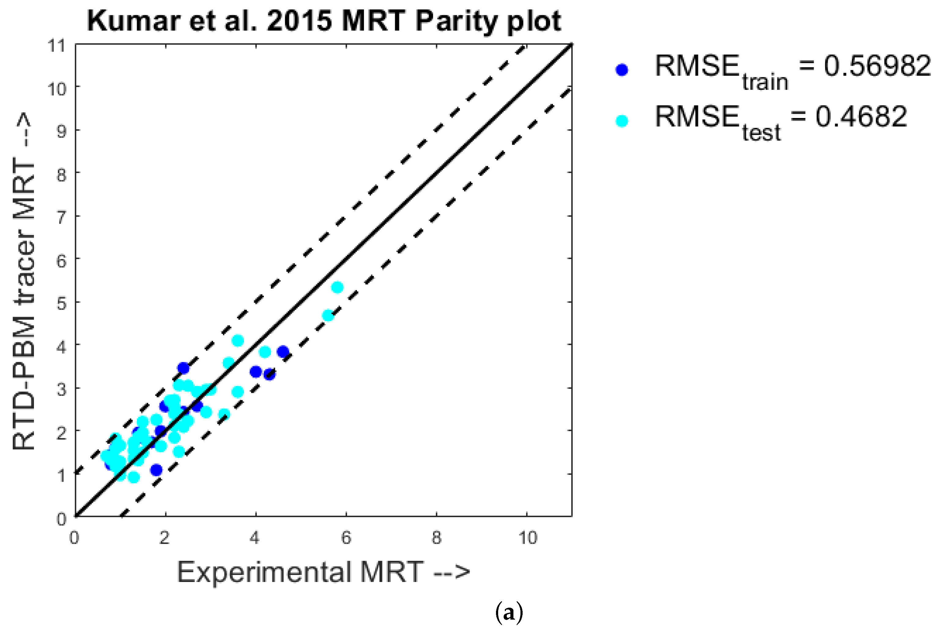
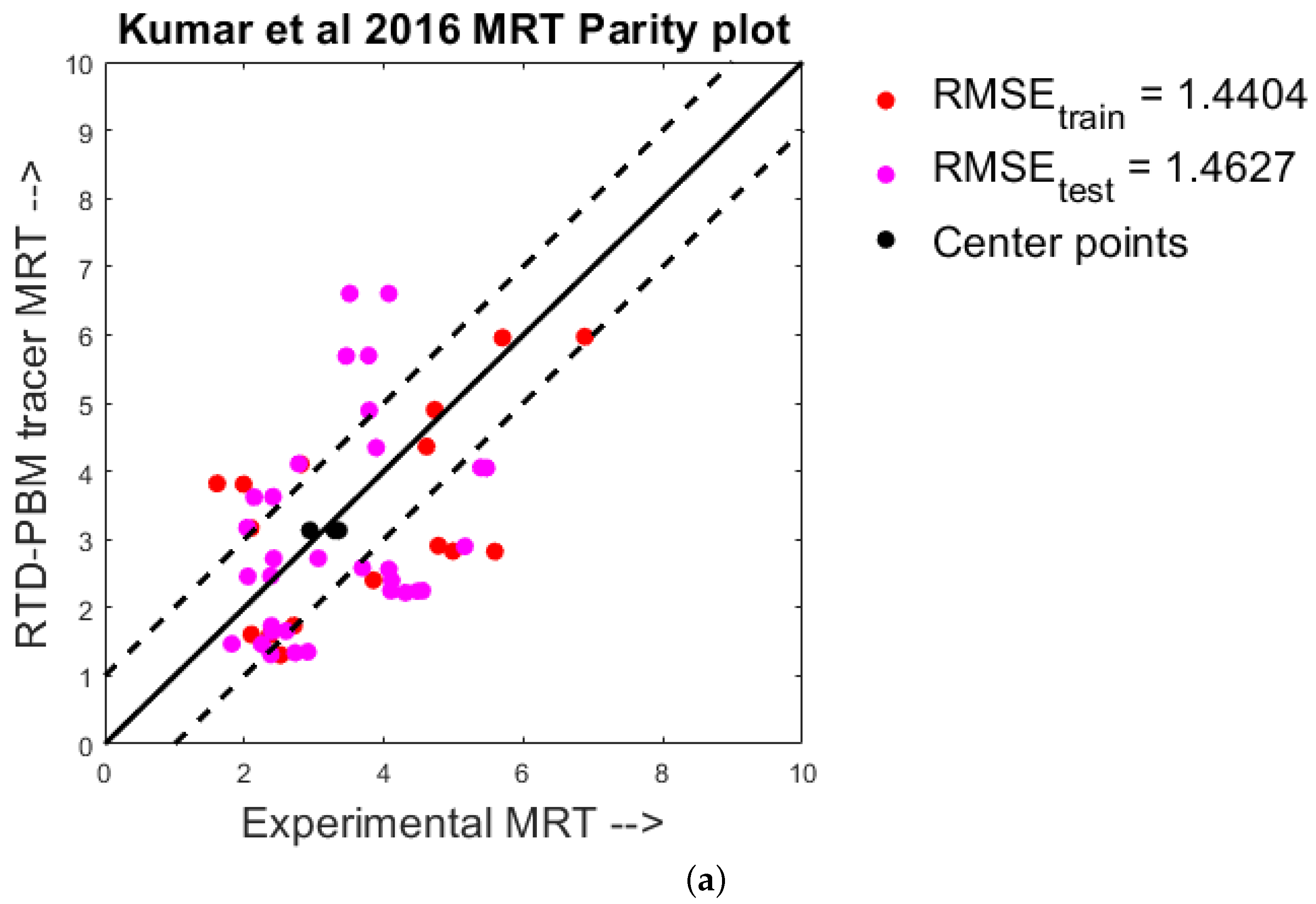
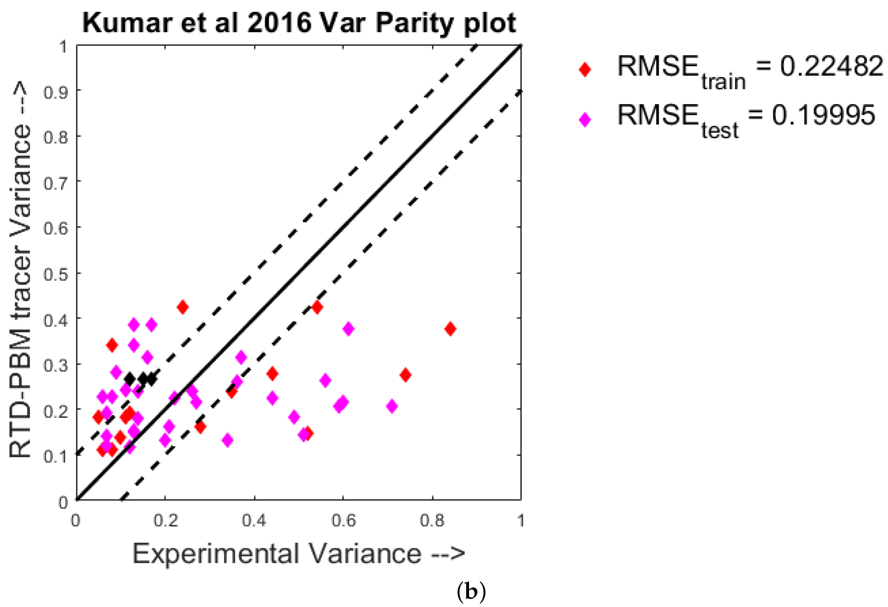
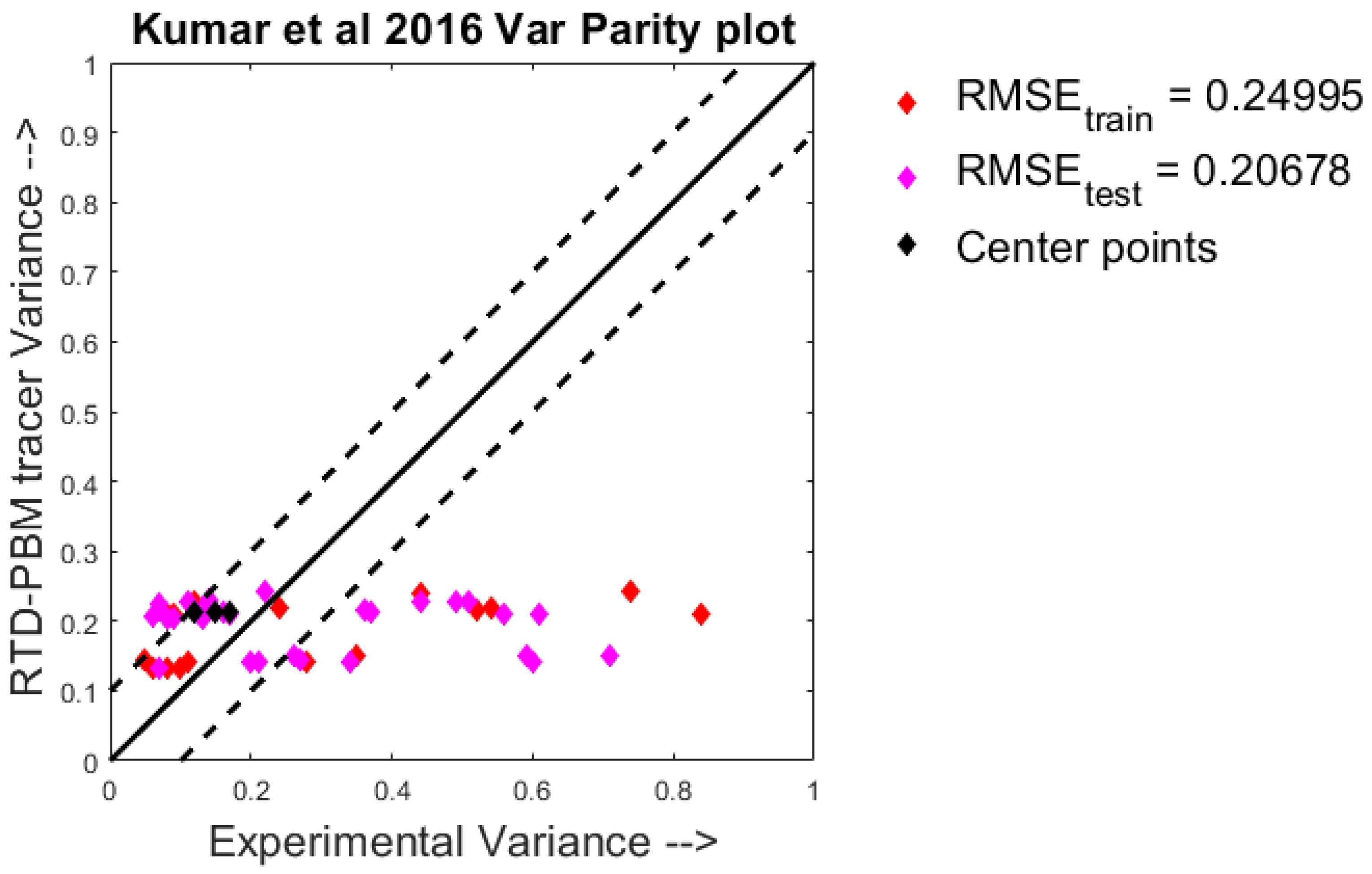
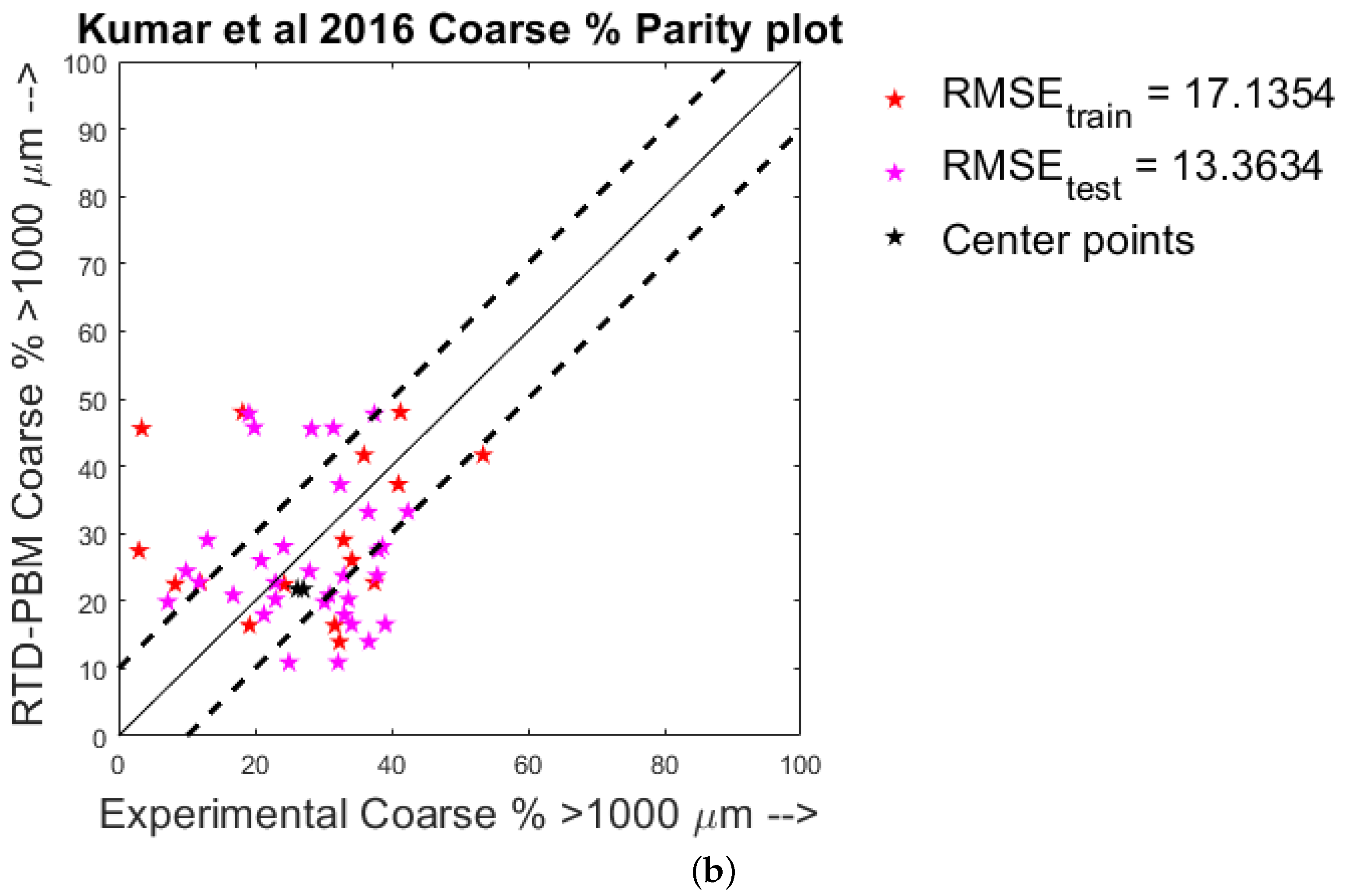
4.1. Quantitative Analysis—Parity Plots

From Figure 3a, it is seen that the model predictions center on either side the $Y=X$ line, with good prediction. All the points lie within the chosen +/−1 confidence interval. From Figure 3b, the model predictions for the normalized variance can be seen where most of the points are scattered between the $Y=X$ and $Y=X-0.1$ line. It can be seen that the predicted variance lies in a range of 0–0.05.

From Figure 4a, it is seen that the model predictions center on either side of side of the $Y=X$ line, although with low precision. However, it is a better prediction than deploying just the residence time model which under-predicted the MRT values as shown in our previous work. From Figure 4b, the model predictions for the normalized variance can be seen, where most of the points are scattered far away either side of the $Y=X$ line. It can be seen that the variance can be predicted in a range of 0.1–0.45, thereby showing limited predictive capability of the variance.

From Figure 5, the model predictions for the normalized variance for a model framework without having any axial dispersion incorporated can be seen. It can be seen that the variance can be predicted in a very narrow range of 0.1–0.2, thereby showing a worse prediction for the variance and thus the necessity of having localised variance dependent dispersion flow.

From Figure 6, it is seen that the model size predictions for the fine granules center lie on the $Y=X$ line, thereby giving a reasonably good prediction.

From Figure 7a, it is seen that the model size predictions for the fine granules center on either side of the $Y=X$ line, with several points lying within the chosen confidence interval of $+/-$10%. From Figure 7b, the model predictions for the coarse granule sizes can be seen, where most of the points are scattered close to the $Y=X$ line, with several scattered within the chosen confidence interval. It can be seen there that a few points have been over-predicted.

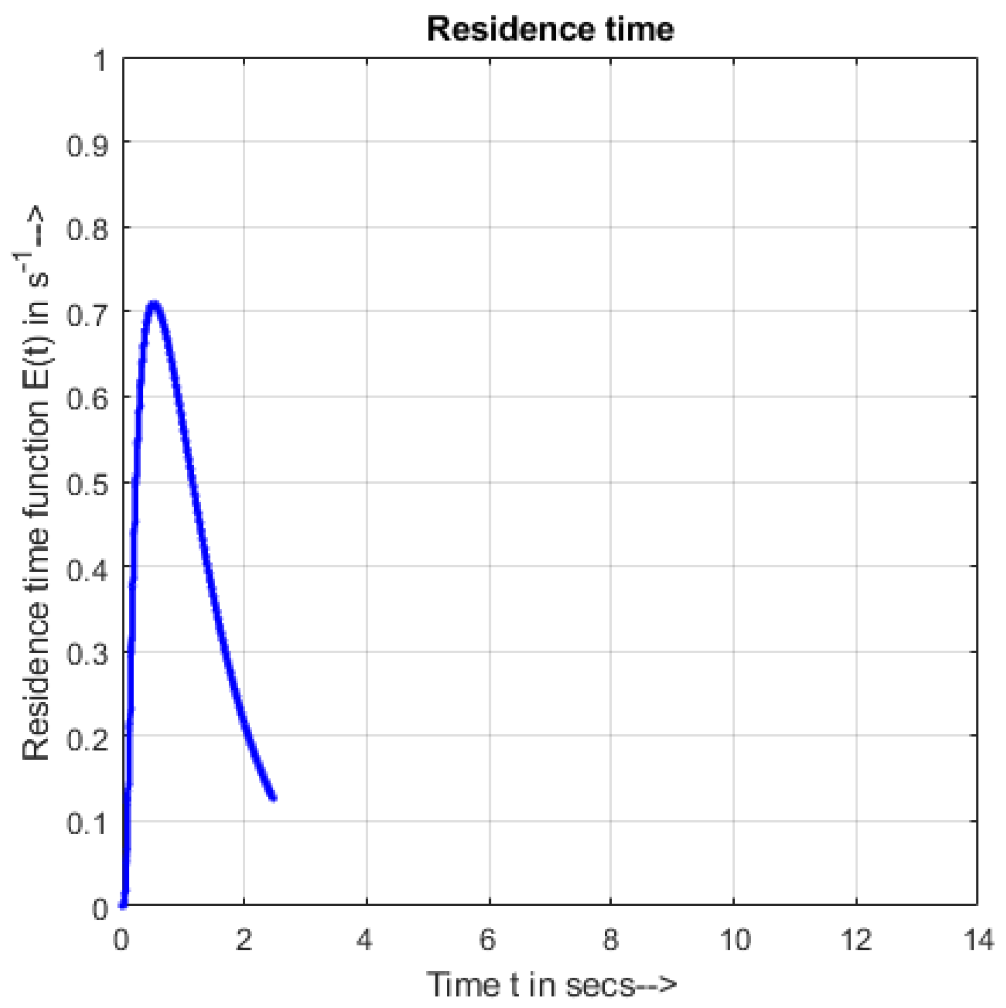
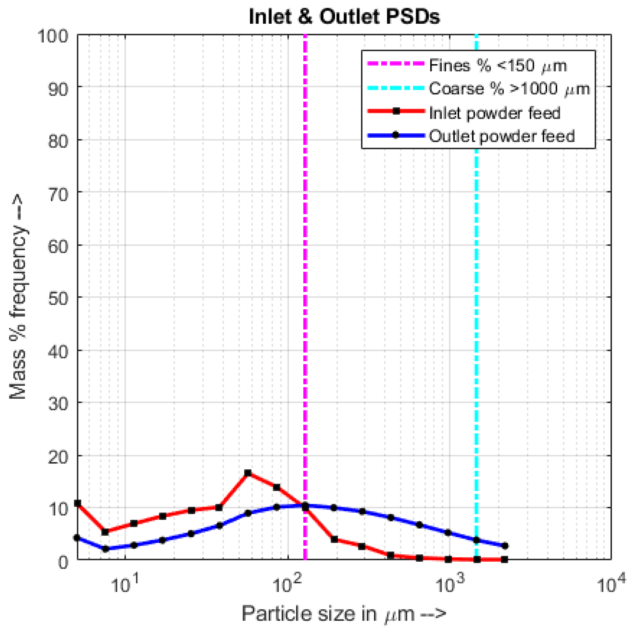
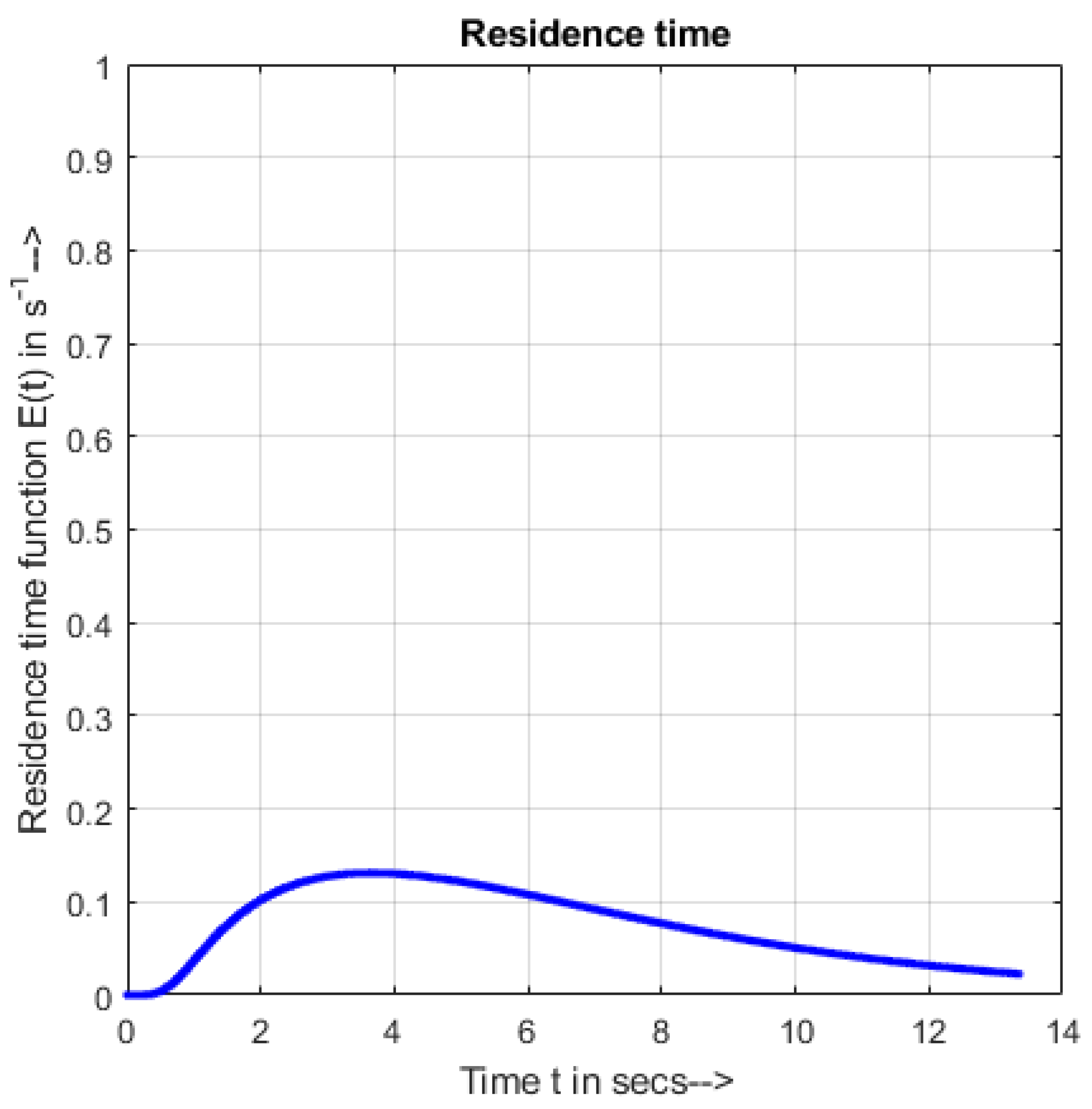
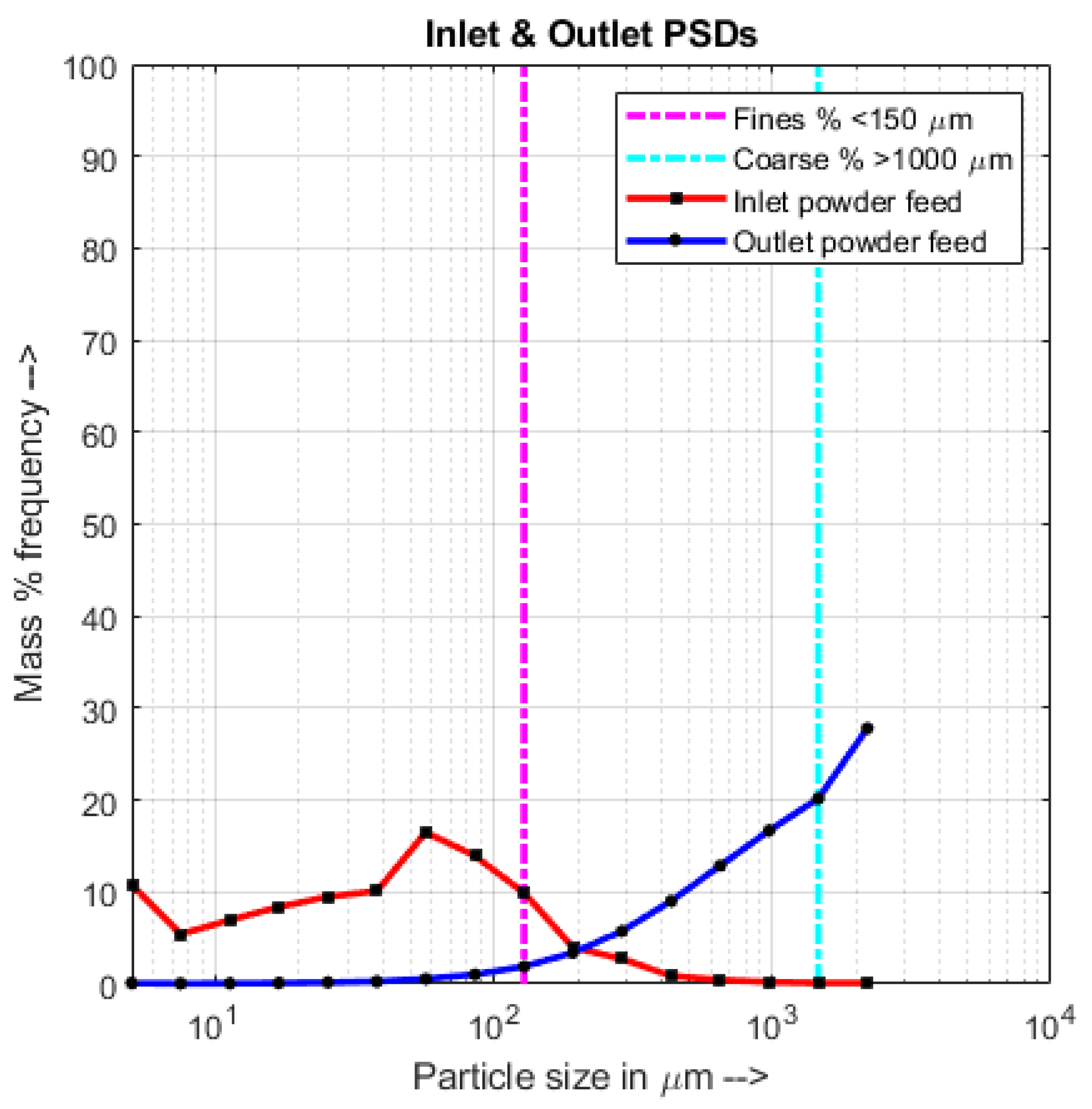
4.2. Qualitative Analysis—Correlation between RTD and PSD

Apart from validating the experimental results by way of parity plots, a combined RTD-PBE framework would also aid in correlating effects of RTD to desirable or undesirable PSD trends in the final granule products.

From Figure 8, it is seen that short residence time was observed for low FR 10 kg/h, low NK $1 \times 4$, low SA ${30}^{\circ }$, and high RPM of 900.

From Figure 9, it is seen that a PSD with the mode of the particle sizes centering at around 100 $\mathsf{\mu }$m was observed for the same run which had a short residence time (low FR 10 kg/h, low NK$1 \times 4$, low SA ${30}^{\circ }$, and high RPM of 900).

From Figure 10, it is seen that a long residence time was observed for high FR 25 kg/h, high NK $2 \times 6$, high SA ${90}^{\circ }$, and low RPM of 900.

From Figure 11, it is seen that a PSD with the the particles rich in larger size fractions for the same run had a long residence time (high FR 25 kg/h, high NK $2 \times 6$, high SA ${60}^{\circ }$, and low RPM of 500).

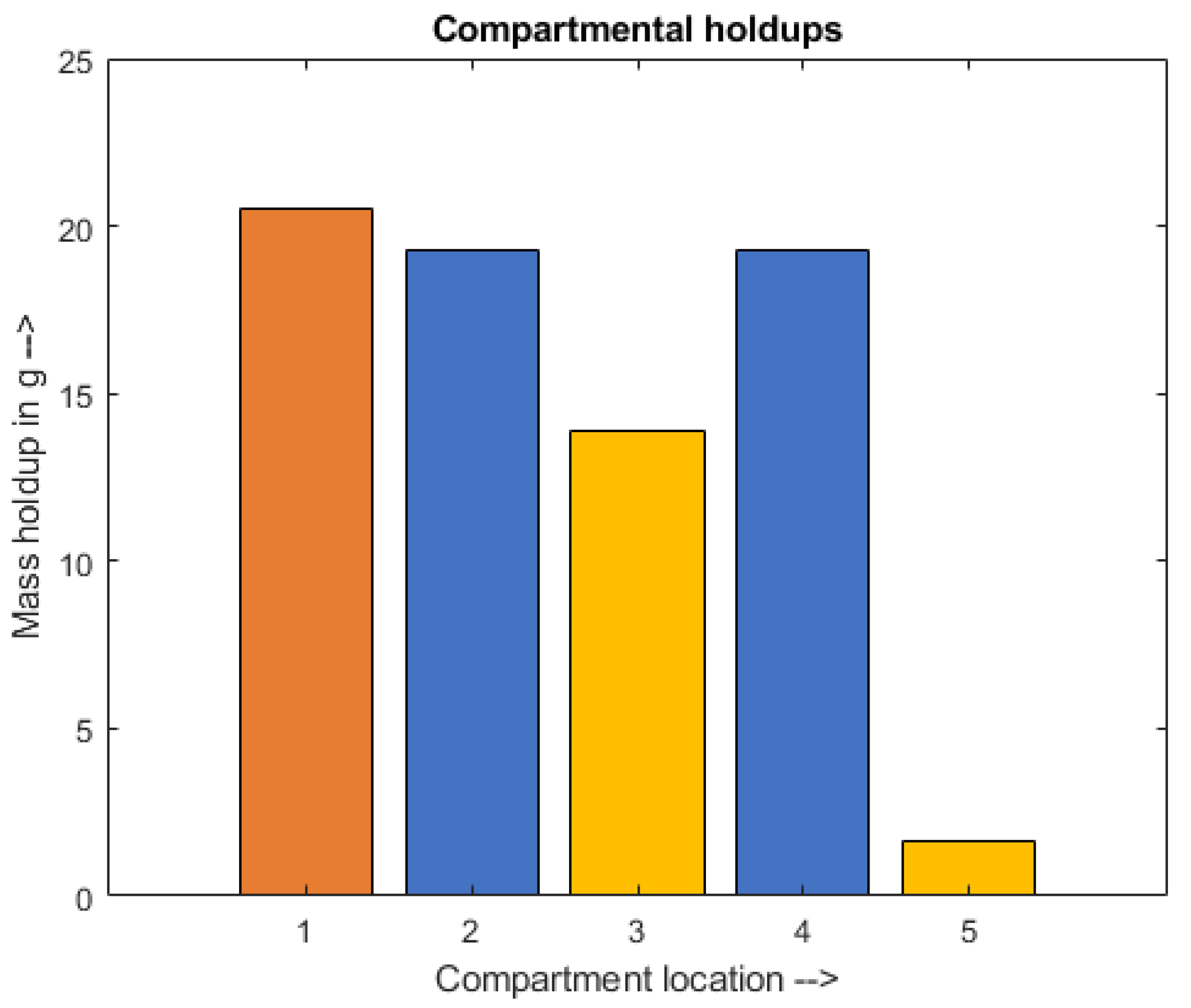
4.3. Qualitative Analysis—Compartmental Holdup

In addition to correlating the RTD of the system to the PSD of the obtained granules, the integrated RTD-PBE framework also gave insights about the compartmental holdup inside the TSG equipment in general.

From Figure 12, it is seen that, in general, the mass holdup in kneading sections (blue bars) is higher than that in the wet conveying screw sections (wet bars). However, in the conveying sections preceding the kneading sections (1—orange bar and 3—1st yellow bar), the compartmental holdups are high due to the backward dispersion flow of granules from the succeeding kneading zones.

5. Conclusions

From the parity plots in Section 4, it is seen that the model performance varies with the distribution of the experimental data-points’ range. The model predicted the experimental MRT and variance fairly well for the Kumar et al., 2015 dataset; however, for several cases in the Kumar et al., 2016, there is either over- or under-prediction. A plausible explanation is that the prediction capability depends on the bounds of the changing process and equipment parameters for different experimental dataset combinations. One plausible reason for the poor prediction for the Kumar et al., 2016 dataset is that the additional process parameter of changing liquid-to-solid percentage is playing a large role in the inherent granulation mechanisms, the incorporation of which would require further study into the granulation kinetics of the specific combination of materials (lactose $\alpha$-monohydrate and theophylline anhydrous). However, incorporating material specific granulation mechanisms to fit the residence times and particle sizes would go against the principle of building generalizable models for twin screw granulation. Moreover, this study focuses more on the incorporation of the previously omitted dispersion flow rates to predict the variances. The presented approach aims to serve as a guiding tool for building population balance models for multi-component twin screw granulation systems which would be useful for predicting the performance in continuous manufacturing lines.

Therefore, in summary, this research paper presents (i) a continuous population balance equation methodology incorporating the axial velocities and dispersion rates separately for each component; (ii) incorporation of previously developed semi-mechanistic expressions for residence time metrics to calculate the axial velocities and dispersion rates; (iii) and lastly validation of the said equations on two different datasets.

References

1. Chaudhury, A.; Kapadia, A.; Prakash, A.V.; Barrasso, D.; Ramachandran, R. An extended cell-average technique for a multi-dimensional population balance of granulation describing aggregation and breakage. Adv. Powder Technol. 2013, 24, 962–971. [Google Scholar] [CrossRef]
2. Chaudhury, A.; Ramachandran, R. Integrated population balance model development and validation of a granulation process. Part. Sci. Technol. 2013, 31, 407–418. [Google Scholar] [CrossRef]
3. Ramachandran, R.; Chaudhury, A. Model-based design and control of a continuous drum granulation process. Chem. Eng. Res. Des. 2012, 90, 1063–1073. [Google Scholar] [CrossRef]
4. Barrasso, D.; Walia, S.; Ramachandran, R. Multi-component population balance modeling of continuous granulation processes: A parametric study and comparison with experimental trends. Powder Technol. 2013, 241, 85–97. [Google Scholar] [CrossRef]
5. Barrasso, D.; El Hagrasy, A.; Litster, J.D.; Ramachandran, R. Multi-dimensional population balance model development and validation for a twin screw granulation process. Powder Technol. 2015, 270, 612–621. [Google Scholar] [CrossRef]
6. Kumar, A.; Vercruysse, J.; Mortier, S.T.; Vervaet, C.; Remon, J.P.; Gernaey, K.V.; De Beer, T.; Nopens, I. Model-based analysis of a twin-screw wet granulation system for continuous solid dosage manufacturing. Comput. Chem. Eng. 2016, 89, 62–70. [Google Scholar] [CrossRef]
7. Shirazian, S.; Darwish, S.; Kuhs, M.; Croker, D.M.; Walker, G.M. Regime-separated approach for population balance modeling of continuous wet granulation of pharmaceutical formulations. Powder Technol. 2018, 325, 420–428. [Google Scholar] [CrossRef]
8. McGuire, A.D.; Mosbach, S.; Lee, K.F.; Reynolds, G.; Kraft, M. A high-dimensional, stochastic model for twin-screw granulation—Part 1: Model description. Chem. Eng. Sci. 2018, 188, 221–237. [Google Scholar] [CrossRef] [Green Version]
9. McGuire, A.D.; Mosbach, S.; Lee, K.F.; Reynolds, G.; Kraft, M. A high-dimensional, stochastic model for twin-screw granulation Part 2: Numerical methodology. Chem. Eng. Sci. 2018, 188, 18–33. [Google Scholar] [CrossRef] [Green Version]
10. Van Hauwermeiren, D.; Verstraeten, M.; Doshi, P.; am Ende, M.T.; Turnbull, N.; Lee, K.; De Beer, T.; Nopens, I. On the modeling of granule size distributions in twin-screw wet granulation: Calibration of a novel compartmental population balance model. Powder Technol. 2019, 341, 116–125. [Google Scholar] [CrossRef]
11. Wang, L.G.; Pradhan, S.U.; Wassgren, C.; Barrasso, D.; Slade, D.; Litster, J.D. A breakage kernel for use in population balance modeling of twin screw granulation. Powder Technol. 2020, 363, 525–540. [Google Scholar] [CrossRef]
12. Lee, K.T.; Ingram, A.; Rowson, N.A. Twin screw wet granulation: The study of a continuous twin screw granulator using Positron Emission Particle Tracking (PEPT) technique. Eur. J. Pharm. Biopharm. 2012, 81, 666–673. [Google Scholar] [CrossRef]
13. Zheng, C.; Zhang, L.; Govender, N.; Wu, C.Y. DEM analysis of residence time distribution during twin screw granulation. Powder Technol. 2020, 377, 924–938. [Google Scholar] [CrossRef]
14. Fogler, H.S. Elements of Chemical Reaction Engineering, 5th ed.; Pearson International Edition; Chapter Models for Nonideal Reactors; Prentice Hall: Hoboken, NJ, USA, 2006; p. 38. [Google Scholar]
15. Barrasso, D.; Ramachandran, R. Qualitative assessment of a multi-scale, compartmental PBM-DEM model of a continuous twin-screw wet granulation process. J. Pharm. Innov. 2016, 11, 231–249. [Google Scholar] [CrossRef]
16. Ge Wang, L.; Morrissey, J.P.; Barrasso, D.; Slade, D.; Clifford, S.; Reynolds, G.; Ooi, J.Y.; Litster, J.D. Model Driven Design for Twin Screw Granulation using Mechanistic-based Population Balance Model. Int. J. Pharm. 2021, 607, 120939. [Google Scholar] [CrossRef]
17. Muddu, S.V.; Kotamarthy, L.; Ramachandran, R. A Semi-Mechanistic Prediction of Residence Time Metrics in Twin Screw Granulation. Pharmaceutics 2021, 13, 393. [Google Scholar] [CrossRef] [PubMed]
18. Kumar, A.; Vercruysse, J.; Vanhoorne, V.; Toiviainen, M.; Panouillot, P.E.; Juuti, M.; Vervaet, C.; Remon, J.P.; Gernaey, K.V.; De Beer, T.; et al. Conceptual framework for model-based analysis of residence time distribution in twin-screw granulation. Eur. J. Pharm. Sci. 2015, 71, 25–34. [Google Scholar] [CrossRef]
19. Kumar, A.; Alakarjula, M.; Vanhoorne, V.; Toiviainen, M.; De Leersnyder, F.; Vercruysse, J.; Juuti, M.; Ketolainen, J.; Vervaet, C.; Remon, J.P.; et al. Linking granulation performance with residence time and granulation liquid distributions in twin-screw granulation: An experimental investigation. Eur. J. Pharm. Sci. 2016, 90, 25–37. [Google Scholar] [CrossRef]
20. Madec, L.; Falk, L.; Plasari, E. modeling of the agglomeration in suspension process with multidimensional kernels. Powder Technol. 2003, 130, 147–153. [Google Scholar] [CrossRef]
21. Pandya, J.; Spielman, L. Floc breakage in agitated suspensions: Effect of agitation rate. Chem. Eng. Sci. 1983, 38, 1983–1992. [Google Scholar] [CrossRef]
22. Portillo, P.M.; Muzzio, F.J.; Ierapetritou, M.G. Using compartment modeling to investigate mixing behavior of a continuous mixer. J. Pharm. Innov. 2008, 3, 161–174. [Google Scholar] [CrossRef]
23. Sen, M.; Singh, R.; Vanarase, A.; John, J.; Ramachandran, R. Multi-dimensional population balance modeling and experimental validation of continuous powder mixing processes. Chem. Eng. Sci. 2012, 80, 349–360. [Google Scholar] [CrossRef]
Figure 1. Schematic showing (a) 7 compartment modeling of equipment for 12 KE configurations; and (b) 4 compartment modeling of equipment for 2, 4, and 6 KE configurations.
Processes 10 00292 g001
Figure 2. Schematic showing the convective and dispersive fluxes entering and leaving a compartment with index ‘i’.
Processes 10 00292 g002
Figure 3. Experimental observations (X) vs. predicted model responses (Y) for RT metrics when model is trained on the Kumar et al., 2015 [18] dataset. (a) MRT; (b) variance.
Processes 10 00292 g003aProcesses 10 00292 g003b
Figure 4. Experimental observations (X) vs. predicted model responses (Y) for RT metrics when the model is trained trained Kumar et al., 2016 [19] dataset. (a) MRT; (b) variance.
Processes 10 00292 g004aProcesses 10 00292 g004b
Figure 5. Experimental observations (X) vs. predicted model responses (Y) for the Variance when the model is trained on the Kumar et al., 2016 [19] dataset without including the dispersion flow rates.
Processes 10 00292 g005
Figure 6. Experimental observations (X) vs. predicted model responses (Y) for outlet bulk granule sizes when the model is trained on the Kumar et al., 2016 [19] dataset.
Processes 10 00292 g006
Figure 7. Experimental observations (X) vs. predicted model responses (Y) for outlet fine and coarse granule sizes when the model is trained on the Kumar et al., 2016 [19] dataset. (a) fines; (b) coarse.
Processes 10 00292 g007aProcesses 10 00292 g007b
Figure 8. RTD trend obtained from a PBM pulse tracer study for an unfavorable granulation case from the experimental DOE of Kumar et al., 2016 [19].
Processes 10 00292 g008
Figure 9. PSD trend obtained from a PBM pulse tracer study for unfavorable granulation case from the DOE of Kumar et al., 2016 [19].
Processes 10 00292 g009
Figure 10. RTD trend obtained from a PBM pulse tracer study for a favorable granulation case from the experimental DOE of Kumar et al., 2016 [19].
Processes 10 00292 g010
Figure 11. Kumar et al., 2016 [19] PSD trend obtained from a PBM pulse tracer study for favorable granulation case.
Processes 10 00292 g011
Figure 12. Compartmental holdup obtained obtained from the PBE model when trained on the system as used by Kumar et al., 2016 dataset [19].
Processes 10 00292 g012