Article

Integral Resonant Controller to Suppress the Nonlinear Oscillations of a Two-Degree-of-Freedom Rotor Active Magnetic Bearing System

1
Department of Physics and Engineering Mathematics, Faculty of Electronic Engineering, Menoufia University, Menouf 32952, Egypt
2
Department of Mathematics and Statistics, College of Science, Taif University, P.O. Box 11099, Taif 21944, Saudi Arabia
3
Department of Automation, Biomechanics and Mechatronics, Faculty of Mechanical Engineering, Lodz University of Technology, 90924 Lodz, Poland
*
Author to whom correspondence should be addressed.
Processes 2022, 10(2), 271; https://doi.org/10.3390/pr10020271
Submission received: 22 December 2021 / Revised: 21 January 2022 / Accepted: 22 January 2022 / Published: 29 January 2022
(This article belongs to the Special Issue Numerical Simulation of Nonlinear Dynamical Systems)

Abstract

:
Within this article, the nonlinear vibration control of the rotor active magnetic bearings system is tackled utilizing the integral resonant controller for the first time. Two integral resonant controllers are proposed to mitigate the system lateral oscillations in the horizontal and vertical directions. Based on the suggested control technique, the whole system dynamical model is derived as a two-degree-of-freedom nonlinear system (i.e., rotor system) coupled linearly to two first-order filters (i.e., the integral resonant controllers). The nonlinear autonomous system that governs the oscillation amplitudes of the controlled system as a function of the control parameters is extracted by applying perturbation analysis. The obtained autonomous system showed that the linear damping coefficients of the rotor system are functions of the control gains, feedback gains, and internal loop feedback gains of the coupled controller. Accordingly, the sensitivity of the rotor oscillation amplitudes to the different control parameters is explored. The stability margins and the optimal control gains are reported via plotting the different stability charts in two-dimensional space. The main acquired results demonstrated that the vibration suppression efficiency of the proposed controller is proportional to the product of both the control and feedback signal gains, and inversely proportional to the square of the internal loop feedback gains. In addition, the analytical investigations confirmed that the proposed integral resonant control method can force the rotor system to respond as a linear one with a single periodic attractor when the control parameters are designed properly. Finally, numerical simulations are performed that have illustrated the excellent correspondence with the obtained analytical results.

1. Introduction

The nonlinear vibration control of the Active Magnetic Bearings System (AMBS) is the main subject of researchers and engineers worldwide due to its huge advantages over the conventional bearings system. The working principle of the magnetic bearings system relies on generating controllable magnetic forces to suspend the rotating shaft in its hovering position without physical contact with the stator. This working mechanism has earned the active magnetic bearings system many benefits over the conventional one such as (1) frictionless operation, (2) no necessity for lubrication, (3) less maintenance, (4) high-speed operation, (5) long working time, (6) clean environment, etc. Therefore, many researchers have investigated the dynamical behaviors of this system, as well as proposed different control strategies to enhance its dynamical stability. Ji et al. [1] studied the nonlinear behaviors of the 4-pole AMBS utilizing the conventional position-velocity feedback control technique. The author investigated the system dynamics in two oscillation modes. Firstly, he explored the system as an autonomous one via neglection of the rotor eccentricity, where the obtained results showed that the AMBS can exhibit saddle-node, saddle-connection, and Hopf bifurcations. Secondly, the author included the effect of the rotor eccentricity in the studied model, where the analysis illustrated that the nonautonomous system may have homoclinic orbit and transversal intersection. Saeed et al. [2,3] investigated the 6-pole AMBS with two different control methods, where they explored the vibration suppression efficiency of a proportional-derivative controller designed based on the Cartesian displacements and Cartesian velocities of the rotor system in [2]. In addition, the performance of a proportional-derivative controller implemented based on the radial displacements and radial velocities has been investigated in [3]. Based on the analysis introduced, they reported that the Cartesian control method has vibration suppression efficiency higher than the radial one. On the other hand, the radial control technique exhibited more stability features than the Cartesian method. The vibration control of the 8-pole AMBS with constant stiffness is investigated in [4,5,6,7,8]. Ji et al. [4,5] studied the position-velocity controller efficiency in suppressing the oscillatory behaviors of an 8-pole system at both the primary and superharmonic resonances. Yang et al. [6] discussed the oscillation modes of the 8-pole AMBS using the energy and phase-difference technique, where the obtained analysis demonstrated that the rotor system can perform either elliptic or quasiperiodic oscillations. Saeed et al. [7] introduced a combination of both the linear and nonlinear position-velocity controllers to enhance the dynamical behaviors of the 8-pole AMBS. They concluded that the integration of a cubic position controller can modify the system oscillatory behavior to respond as a hardening or softening spring oscillator. Saeed et al. [8] investigated the effect of rub-impact force on motion bifurcation of the 8-pole AMBS. The authors explored the nature of system motion utilizing both the impact stiffness and the dynamic friction coefficients as the bifurcation parameters. They reported that the system can oscillate with one of three vibration modes, which are (a) full annular rub, (b) period-n rub-impact, and (c) and quasiperiodic rub-impact. The efficiency of a time-varying proportional-derivative controller in mitigating the nonlinear vibrations of the 8-pole AMBS is introduced by Zhang et al. [9,10,11,12,13,14]. Based on the investigations introduced, they reported that the system exhibits Shilnikov multipulse chaotic motion. Furthermore, the system can oscillate with periodic-n, quasiperiodic, and chaotic motion. El-Shourbagy et al. [15] explored the oscillatory motion of the 12-pole AMBS for the first time utilizing the conventional PD-controller, where the authors reported that the proportional gain can play an important role in reshaping the system dynamics. Different control methodologies to control the 16-pole AMBS have been introduced [16,17,18,19,20,21]. Saeed and Kandil [16] utilized the PD-controller with two configuration methods to suppress the nonlinear vibrations of the 16-pole AMBS. The authors implemented the proposed control based on both the Cartesian and radial displacements and velocities of the rotor system. They found that the Cartesian control can suppress vibrations better than the radial control technique, while the radial control has higher stability characteristics than the Cartesian one. Zhang et al. [17,18,19,20,21] investigated the bifurcation behaviors of the 16-pole system utilizing time time-varying PD-controller. The reliability and durability features of the active magnetic bearing system made many of the researchers use it not only as a replacement for the conventional bearings system but also as an active actuator with advanced control algorithms to control the lateral vibrations in different rotating machinery [22,23,24,25,26,27].
The Integral Resonant Controller (IRC) proved its capability in suppressing the nonlinear oscillations and eliminating the catastrophic bifurcation behaviors for different categories of the dynamical systems [28,29,30,31,32,33,34]. Diaz et al. [28] control the vibrations of a lightweight structure utilizing IRC. Al-Mamun et al. [29] investigated the resonant vibrations control of a piezoelectric micro-actuator utilized the integral resonant controller. The authors concluded that the IRC is the best compared to the conventional control method and the use of a notch filter. Omidi and Mahmoodi [30], and MacLean and Sumeet [31] introduced modified versions of the IRC to control the transversal oscillation of a smart structure, where the obtained results demonstrated the efficiency of the applied controller. Omidi and Mahmoodi [32,33] integrated the IRC along with the Positive Position Feedback Controller (PPFC) to mitigate the primary resonance of a nonlinear flexible structure. The authors concluded that the IRC has high efficiency in suppressing the response peaks due to the PPFC. Recently, Saeed et al. [34] employed the nonlinear integral resonant controller with time delays to eliminate the principal parametric oscillation of a vertically suspended cantilever beam system. The authors showed that the introduced control method can mitigate the system oscillation amplitude to zero. Despite the high efficiency of the IRC in suppressing the nonlinear oscillations of different dynamical systems [28,29,30,31,32,33,34], it is not applied before to control the lateral vibrations of the magnetic bearing system [1,2,3,4,5,6,7,8,9,10,11,12,13,14,15,16,17,18,19,20,21,22,23,24,25,26,27].
Within this work, the integral resonant controller has been introduced within this article as a new control strategy to mitigate the nonlinear oscillations of the 8-pole rotor active magnetic bearings system for the first time. Two integral resonant controllers are coupled to the 8-pole rotor system to suppress its horizontal and vertical oscillations. According to the proposed control method, the system equations of motion are derived relying on the principle of classical mechanics. The perturbation analysis is utilized to extract the controlled system amplitude-phase modulating equations. Then, the different response curves and stability charts are plotted. The influence of the different control gains on the system lateral vibrations is explored, and the system stability margins are reported. The main obtained results demonstrated that the linear damping coefficients of the rotor system are proportional to the product of both the control and feedback signal gains (i.e., η 1   η 3 and η 2   η 4 ), and inversely proportional to the square of the internal loop feedback gains (i.e., λ 1 2 and λ 2 2 ) of the coupled IRC controllers. In addition, it is reported that the IRC can force the rotor system to vibrate as a linear one with negligible oscillation amplitudes if the control parameters have been tuned properly.

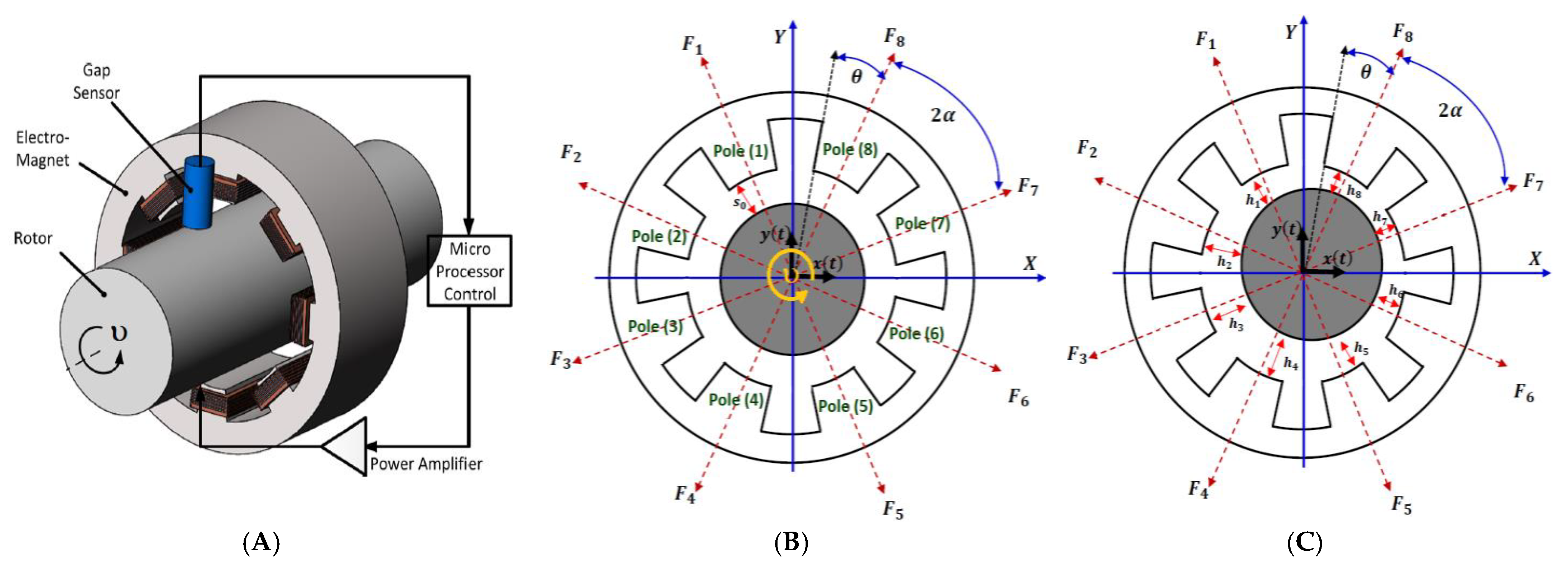
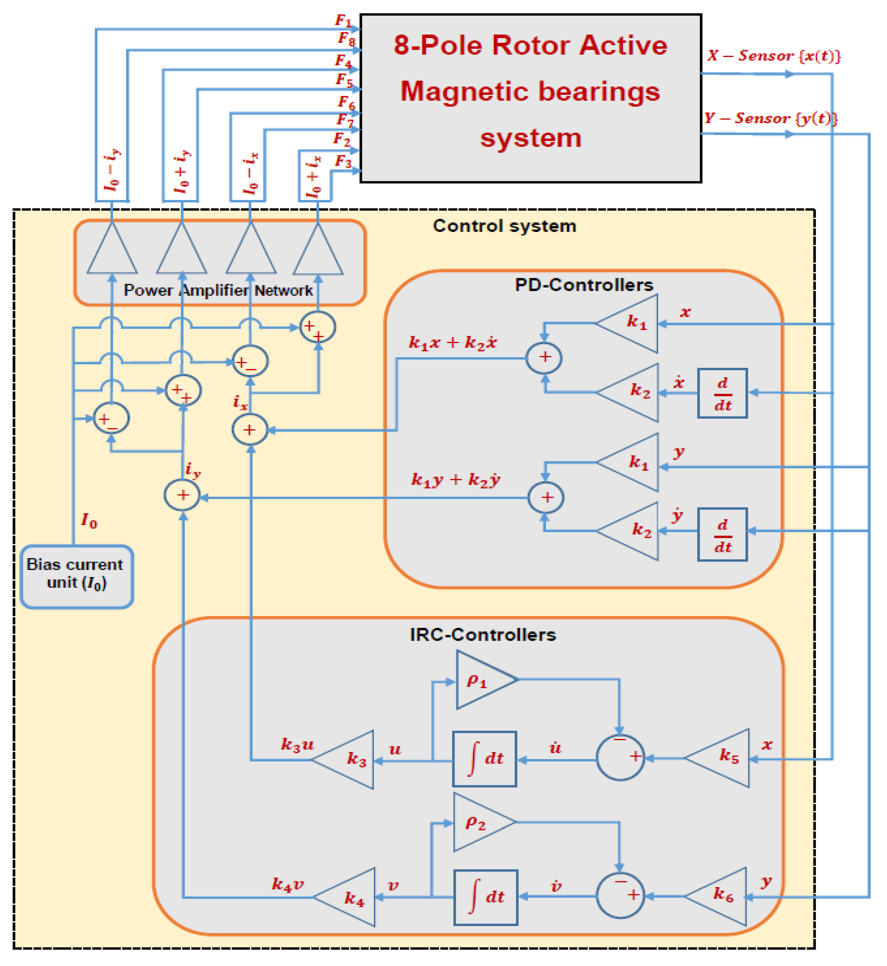
2. Mathematical Modelling

This section is dedicated to obtaining the mathematical model of the eight-pole system that is controlled by both proportional-derivative and integral resonant controllers. The rotor system is modeled as shown in Figure 1 as a two-degree-of-freedom system that performs instantaneous displacements x ( t ) and y ( t ) in X and Y directions when spinning with angular speed υ about its axes. In addition, eight identical electromagnetic poles are utilized as an actuator to control the system oscillations via producing control force based on a predefined control law. Accordingly, the system equations of motions can be written as follows [35,36]:
m x ¨ ( t ) = m e υ 2 cos ( υ t ) + F X C
m y ¨ ( t ) = m e υ 2 sin ( υ t ) + F Y C
where m is the system mass, x ( t ) and y ( t ) are the temporal oscillations of the system in X and Y directions, υ denotes the system angular speed, e is the eccentricity of the rotor, F X C , F Y C represent the net control forces that are generated via the eight electromagnetic poles to mitigate the rotor oscillations in X and Y directions. According to the electromagnetic theory [36], the electromagnetic attractive forces F j ,   ( j = 1 , 2 , 3 , , 8 ) of the eight poles shown in Figure 1B can be expressed as follows:
F j = Δ I j 2 h j 2 , j = 1 , 2 , , 8
where Δ is constant such that Δ = 1 4 µ 0 N 2 A   cos ( θ ) ( µ 0 denotes the air-gap permeability, N is the coil turn number of each pole, A   cos ( θ ) is the effective cross-sectional area), I j denotes the electrical current in ampere of the j th pole, h j represent the instantaneous air gap size as shown in Figure 1B. Let s 0 be the nominal air gap of the rotor system, and 2 α be the angle between every two consecutive poles as shown in Figure 1B. So, for the small deviations x ( t ) and y ( t ) of the rotor, the instantaneous air gap size h j can be expressed as follows:
h j = s 0 ± x sin ( α ) y cos ( α ) , j = 1 , 5 h j = s 0 ± x sin ( α ) ± y cos ( α ) , j = 4 , 8 h j = s 0 ± x cos ( α ) y sin ( α ) , j = 2 , 6 h j = s 0 ± x cos ( α ) ± y sin ( α ) , j = 3 , 7 }
According to the schematic diagram shown in Figure 1C, the eight poles current ( I 1 ,   I 2 ,   ,   I 8 ) can be proposed such that:
I 1 ( t ) = I 8 ( t ) = I 0 i y ( t ) , I 2 ( t ) = I 3 ( t ) = I 0 + i x ( t ) , I 4 ( t ) = I 5 ( t ) = I 0 + i y ( t ) , I 6 ( t ) = I 7 ( t ) = I 0 i x ( t ) . }
where I 0 is constant current, and i x ( t ) and i y ( t ) are the control currents that depend on the proposed control law. Within this work, a combination of both the linear proportional-derivative controller and the integral resonant controller (i.e., PD + IRC controllers) are suggested to control the nonlinear vibrations of the rotor AMB system for the first time. Therefore, the currents i x ( t ) and i y ( t ) are designed such that:
i x ( t ) = k 1 x ( t ) + k 2 x ˙ ( t ) + k 3 u ( t ) , i y ( t ) = k 1 y ( t ) + k 2 y ˙ ( t ) + k 4 v ( t )
where k 1 is the linear proportional gain, k 2 denotes the linear derivative gain, k 3 represents the control gain of the integral resonant controller that is coupled to the horizontal vibration mode x ( t ) , and k 4 is the control gain of the integral resonant controller that is coupled to the vertical vibration mode y ( t ) .
Accordingly, the proposed integral resonant controllers are modeled as linear first-order filters as follows [28,29,30,31,32,33,34]:
u ˙ ( t ) + ρ 1 u ( t ) = k 5 x ( t )
v ˙ ( t ) + ρ 2 v ( t ) = k 6 y ( t )
where u ( t ) and u ˙ ( t ) denote the displacement and velocity of the IRC that is connected to the horizontal vibration mode. v ( t ) and v ˙ ( t ) denote the displacement and velocity of the IRC that connected to the vertical vibration mode. ρ 1 ,   ρ 2 are constants, k 5 ,   k 6 are the feedback control gains. Figure 2 shows the engineering implementation of the proposed control strategy in more detail.
Now, by substituting Equations (4)–(6) into Equation (3), we have
F 1 = Δ ( I 0 k 1 y k 2 y ˙ k 4 v s 0 + x sin ( α ) y cos ( α ) ) 2 , F 2 = Δ ( I 0 + k 1 x + k 2 x ˙ + k 3 u s 0 + x cos ( α ) y sin ( α ) ) 2 , F 3 = Δ ( I 0 + k 1 x + k 2 x ˙ + k 3 u s 0 + x cos ( α ) + y sin ( α ) ) 2 , F 4 = Δ ( I 0 + k 1 y + k 2 y ˙ + k 4 v s 0 + x sin ( α ) + y cos ( α ) ) 2 , F 5 = Δ ( I 0 + k 1 y + k 2 y ˙ + k 4 v s 0 x sin ( α ) + y cos ( α ) ) 2 , F 6 = Δ ( I 0 k 1 x k 2 x ˙ k 3 u s 0 x cos ( α ) + y sin ( α ) ) 2 , F 7 = Δ ( I 0 k 1 x k 2 x ˙ k 3 u s 0 x cos ( α ) y sin ( α ) ) 2 , F 8 = Δ ( I 0 k 1 y k 2 y ˙ k 4 v s 0 x sin ( α ) y cos ( α ) ) 2 }
Based on the system geometry shown in Figure 1B, the net control forces F X C and F Y C in X and Y directions, can be expressed such that:
F X C = ( F 6 + F 7 F 2 F 3 ) cos ( α ) + ( F 5 + F 8 F 1 F 4 ) sin ( α )
F Y C = ( F 1 + F 8 F 4 F 5 ) cos ( α ) + ( F 2 + F 7 F 3 F 6 ) sin ( α )
Expanding Equations (10) and (11) using Taylor series up to third-order approximation as given in Appendix A, and then substituting the resulting equations into Equations (1) and (2) with introducing the dimensionless variables and parameter   t * = ω n t ,   x * = x s 0 ,   y * = y s 0 ,   u * = u s 0 ,   v * = v s 0 ,   p = s 0 I 0 k 1 ,   d = s 0 ω n I 0 k 2 ,   η 1 = 8 cos ( α ) s 0 I 0 k 3 ,   η 2 = 8 cos ( α ) s 0 I 0 k 4 ,   η 3 = k 5 ω n ,   η 4 = k 6 ω n ,   λ 1 = ρ 1 ω n ,   λ 2 = ρ 2 ω n ,   f = e s 0 ,   Ω = υ ω n ,   ω n = Δ / m s 0 3 , we get the equations of motion (after neglecting the asterisks for brevity) as follows:
x ¨ + 2 μ x ˙ + ω 2 x ( α 1 x 3 + α 2 x y 2 + α 3 x 2 x ˙ + α 4 x ˙ y 2 + α 5 x y ˙ 2 + α 6 x x ˙ 2 + α 7 x y y ˙ + β 1 x 2 u + β 2 x x ˙ u + β 3 x u 2 + β 4 x y v + β 5 x v 2 + β 6 x y ˙ v + β 7 u y 2 ) = Ω 2 f cos ( Ω t ) + η 1 u
y ¨ + 2 μ y ˙ + ω 2 y - ( α 1 y 3 + α 2 y x 2 + α 3 y 2 y ˙ + α 4 y ˙ x 2 + α 5 y x ˙ 2 + α 6 y y ˙ 2 + α 7 y x x ˙ + γ 1 y 2 v + γ 2 y y ˙ v + γ 3 y v 2 + γ 4 y x u + γ 5 y u 2 + γ 6 y x ˙ u + γ 7 v x 2 ) = Ω 2 f sin ( Ω t ) + η 2 v
u ˙ + λ 1 u = η 3 x
v ˙ + λ 2 v = η 4 y
where the coefficients μ ,   ω ,   α j ,   β j ,   γ j ,   j = 1 , 2 , , 7 are given in Appendix B. Equations (12)–(15) represent the whole governing equations of motion of the controlled rotor system, where Equations (12) and (13) represent the equations of motion of the controlled rotor system, and Equations (14) and (15) are the equations of motion of the connected integral resonant controllers.

3. Analytical Investigations

To investigate the performance of the proposed control law (i.e., IRC controllers), the multiple scales perturbation method is applied within this section to obtain the periodic solutions of the nonlinear dynamical system given by Equations (12)–(15). Accordingly, the first-order approximate solution to Equations (12)–(15) is proposed as follows [37,38]:
x ( t , ε ) = x 0 ( T 0 , T 1 ) + ε x 1 ( T 0 , T 1 )
y ( t , ε ) = y 0 ( T 0 , T 1 ) + ε y 1 ( T 0 , T 1 )
u ( t , ε ) = ε u 0 ( T 0 , T 1 ) + ε 2 u 1 ( T 0 , T 1 )
v ( t , ε ) = ε v 0 ( T 0 , T 1 ) + ε 2 v 1 ( T 0 , T 1 )
where ε is an artificial parameter used as a book-keeping only [38], T 0 = t , and T 1 = ε t . Accordingly, the derivatives d d t and d 2 d t 2 can be expressed in terms of T 0 and T 1 as follows:
d d t = D 0 + ε D 1 ,   d 2 d t 2 = D 0 2 + 2 ε D 0 D 1 , D j = T j , j = 0 , 1  
To obtain the system solution using the multiple scales method, the system parameters should be scaled such that:
μ = ε μ ^ , f = ε f ^ , α j = ε α ^ j , η 3 = ε η ^ 3 , η 4 = ε η ^ 4 , j = 1 , , 7
Substituting Equations (16)–(21) into Equations (12) and (15) with equating the coefficients that have the same power of ε , we get
O ( ε 0 ):
( D 0 2 + ω 2 ) x 0 = 0
( D 0 2 + ω 2 ) y 0 = 0
O ( ε ):
( D 0 + λ 1 ) u 0 = η ^ 3 x 0
( D 0 + λ 2 ) v 0 = η ^ 4 y 0
( D 0 2 + ω 2 ) x 1 = 2 D 0 D 1 x 0 2 μ ^ D 0 x 0 + α ^ 1 u 0 3 + α ^ 2 x 0 y 0 2 + α ^ 3 x 0 2 D 0 x 0 + α ^ 4 y 0 2 D 0 x 0 + α ^ 5 x 0 ( D 0 y 0 ) 2 + α ^ 6 x 0 ( D 0 x 0 ) 2 + α ^ 7 x 0 y 0 D 0 y 0 + β 1 x 0 2 u 0 + β 2 x 0 D 0 x 0 u 0 + β 3 x 0 u 0 2 + β 4 x 0 y 0 v 0 + β 5 x 0 v 0 2 + β 6 x 0 D 0 y 0 v 0 + β 7 y 0 2 u 0 + Ω 2 f ^ cos ( Ω t ) + η 1 u 0
( D 0 2 + ω 2 ) y 1 = 2 D 0 D 1 y 0 2 μ ^ D 0 y 0 + α ^ 1 y 0 3 + α ^ 2 y 0 x 0 2 + α ^ 3 y 0 2 D 0 y 0 + α ^ 4 x 0 2 D 0 y 0 + α ^ 5 y 0 ( D 0 x 0 ) 2 + α ^ 6 y 0 ( D 0 y 0 ) 2 + α ^ 7 y 0 x 0 D 0 x 0 + γ 1 y 0 2 v 0 + γ 2 y 0 D 0 y 0 v 0 + γ 3 y 0 v 0 2 + γ 4 y 0 x 0 u 0 + γ 5 y 0 u 0 2 + γ 6 y 0 D 0 x 0 u 0 + γ 7 x 0 2 v 0 + Ω 2 f ^ sin ( Ω t ) + η 2 v 0
The steady-state solution of Equations (22)–(25) can be expressed as follows:
x 0 ( T 0 , T 1 ) = A ( T 1 ) e i ω T 0 + A ¯ ( T 1 ) e i ω T 0
y 0 ( T 0 , T 1 ) = B ( T 1 ) e i ω T 0 + B ¯ ( T 1 ) e i ω T 0
u 0 ( T 0 , T 1 ) = δ 1 A ( T 1 ) e i ω T 0 + δ ¯ 1 A ¯ ( T 1 ) e i ω T 0
v 0 ( T 0 , T 1 ) = δ 2 B ( T 1 ) e i ω T 0 + δ ¯ 2 B ¯ ( T 1 ) e i ω T 0
where i = 1 ,   δ 1 = λ 1 i ω λ 1 2 + ω 2 η ^ 3 ,   δ 2 = λ 2 i ω λ 2 2 + ω 2 η ^ 4 , and A ( T 1 ) , B ( T 1 ) are unknown functions that will be determined later. By substituting Equations (28)–(31) into Equations (26) and (27), we have
( D 0 2 + ω 2 ) x 1 = [ 2 i ω ( D 1 A ) 2 i μ ^ ω A + 3 α ^ 1 A 2 A ¯ + 2 α ^ 2 A B B ¯ + α ^ 2 A ¯ B 2 + i α ^ 3 ω A 2 A ¯ + 2 i α ^ 4 ω A B B ¯ i α ^ 4 ω A ¯ B 2 + 2 α ^ 5 ω 2 A B B ¯ α ^ 5 ω 2 A ¯ B 2 + α ^ 6 ω 2 A 2 A ¯ + i α ^ 7 ω A ¯ B 2 + 2 β 1 δ 1 A 2 A ¯ + β 3 δ 1 2 A 2 A ¯ + β 4 ( δ 2 A B B ¯ + δ 2 A ¯ B 2 ) + β 5 δ 2 2 A ¯ B 2 + β 6 ( i ω δ 2 A B B ¯ + i ω δ 2 A ¯ B 2 ) + 2 β 7 δ 1 A B B ¯ + η 1 δ 1 A ] e i ω T 0 + [ α ^ 1 A 3 + α ^ 2 A B 2 + i α ^ 3 ω A 3 + i α ^ 4 ω A B 2 α ^ 5 ω 2 A B 2 α ^ 6 ω 2 A 3 + i α ^ 7 ω A B 2 + β 1 δ 1 A 3 + i β 2 ω δ 1 A 3 e 3 i ω T 0 + β 3 δ 1 2 A 3 e 3 i ω T 0 + β 4 δ 2 A B 2 + β 5 δ 2 2 A B 2 + i β 6 ω δ 2 A B 2 + β 7 δ 1 A B 2 ] e 3 i ω T 0 + 1 2 Ω 2 f ^ e i Ω T 0 + c c
( D 0 2 + ω 2 ) y 1 = [ 2 i ω ( D 1 B ) 2 i μ ^ ω B + 3 α ^ 1 B 2 B ¯ + 2 α ^ 2 B A A ¯ + α ^ 2 B ¯ A 2 + i α ^ 3 ω B 2 B ¯ + 2 i α ^ 4 ω B A A ¯ i α ^ 4 ω B ¯ A 2 + 2 α ^ 5 ω 2 B A A ¯ α ^ 5 ω 2 B ¯ A 2 + α ^ 6 ω 2 B 2 B ¯ + i α ^ 7 ω B ¯ A 2 + 2 γ 1 δ 1 B 2 B ¯ + γ 3 δ 2 2 B 2 B ¯ + γ 4 ( δ 1 B A A ¯ + δ 1 B ¯ A 2 ) + γ 5 δ 1 2 B ¯ A 2 + γ 6 ( i ω δ 1 B A A ¯ + i ω δ 1 B ¯ A 2 ) + 2 γ 7 δ 1 B A A ¯ + η 2 δ 1 B ] e i ω T 0 + [ α ^ 1 B 3 + α ^ 2 B A 2 + i α ^ 3 ω B 3 + i α ^ 4 ω B A 2 α ^ 5 ω 2 B A 2 α ^ 6 ω 2 B 3 + i α ^ 7 ω B A 2 + γ 1 δ 1 B 3 + i γ 2 ω N B 3 e 3 i ω T 0 + γ 3 δ 2 2 B 3 + γ 4 δ 1 B A 2 e 3 i ω T 0 + γ 5 δ 1 2 B A 2 + i γ 6 ω δ 1 B A 2 + γ 7 δ 1 B A 2 ] e 3 i ω T 0 1 2 i Ω 2 f ^ e i Ω T 0 + c c
where c c denotes the complex conjugate term. To obtain the solvability conditions of Equations (32) and (33), the closeness of the rotor spinning speed ( Ω ) to the system natural frequency ( ω ) is described via introducing the detuning parameter σ as follows:
Ω = ω + σ = ω + ε σ ^
Substituting Equation (34) into Equations (32) and (33), one can obtain the following solvability conditions:
2 i ω ( D 1 A ) 2 i μ ^ ω A + 3 α ^ 1 A 2 A ¯ + 2 α ^ 2 A B B ¯ + α ^ 2 A ¯ B 2 + i ω α ^ 3 A 2 A ¯ + 2 i ω α ^ 4 A B B ¯ i ω α ^ 4 A ¯ B 2 + 2 ω 2 α ^ 5 A B B ¯ ω 2 α ^ 5 A ¯ B 2 + ω 2 α ^ 6 A 2 A ¯ + i ω α ^ 7 A ¯ B 2 + 2 β 1 δ 1 A 2 A ¯ + β 3 δ 1 2 A 2 A ¯ + β 4 δ 2 A B B ¯ + β 4 δ 2 A ¯ B 2 + β 5 δ 2 2 N 2 A ¯ B 2 i ω β 6 δ 2 A B B ¯ + i ω β 6 δ 2 A ¯ B 2 + 2 β 7 δ 1 A B B ¯ + η 1 δ 1 A + 1 2 ( ω + σ ) 2 f ^ e i ε σ ^ T 0 = 0
2 i ω ( D 1 B ) 2 i μ ^ ω B + 3 α ^ 1 B 2 B ¯ + 2 α ^ 2 B A A ¯ + α ^ 2 B ¯ A 2 + i ω α ^ 3 B 2 B ¯ + 2 i ω α ^ 4 B A A ¯ i ω α ^ 4 B ¯ A 2 + 2 ω 2 α ^ 5 B A A ¯ ω 2 α ^ 5 B ¯ A 2 + ω 2 α ^ 6 B 2 B ¯ + i ω α ^ 7 B ¯ A 2 + 2 γ 1 δ 2 B 2 B ¯ + γ 3 δ 2 2 B 2 B ¯ + γ 4 δ 1 B A A ¯ + γ 4 δ 1 B ¯ A 2 + γ 5 δ 1 2 B ¯ A 2 i ω γ 6 δ 1 B A A ¯ + i ω γ 6 δ 1 B ¯ A 2 + 2 γ 7 δ 2 B A A ¯ + η 2 δ 2 B 1 2 i ( ω + σ ) 2 f ^ e i ε σ ^ T 0 = 0
To obtain the amplitude-phase equations of the controlled system, the functions A ( T 1 ) and B ( T 1 ) can be expressed in the polar form as follows:
A ( T 1 ) = 1 2 a ( T 1 ) e i θ 1 ( T 1 ) , B ( T 1 ) = 1 2 b ( T 1 ) e i θ 2 ( T 1 )
Substituting Equation (37) into Equations (35) and (36), and then separating the real and imaginary parts, we have the following amplitude-phase modulating equations:
a ˙ = G 1 ( a , b , φ 1 , φ 2 ) = ( μ + η 3 η 1 2 ( λ 1 2 + ω 2 ) ) a + 1 8 ( α 3 2 β 1 η 3 λ 1 2 + ω 2 2 β 3 λ 1 η 3 2 ( λ 1 2 + ω 2 ) 2 ) a 3 + 1 8 ( 2 α 4 β 4 η 4 λ 2 2 + ω 2 β 6 λ 2 η 4 λ 2 2 + ω 2 2 β 7 η 3 λ 1 2 + ω 2 ) a b 2 + 1 8 ( α 4 + α 7 β 4 η 4 λ 2 2 + ω 2 + 2 β 5 λ 2 η 4 2 ( λ 2 2 + ω 2 ) 2 + β 6 λ 2 η 4 λ 2 2 + ω 2 ) a b 2 cos ( 2 φ 2 2 φ 1 ) 1 8 ( α 2 ω α 5 ω + β 4 η 4 λ 2 ω ( λ 2 2 + ω 2 ) + β 5 η 4 2 ( λ 2 2 ω 2 ) ω ( λ 2 2 + ω 2 ) 2 β 6 η 4 ω λ 2 2 + ω 2 ) a b 2 sin ( 2 φ 2 2 φ 1 ) + f 2 ω ( ω + σ ) 2 sin ( φ 1 )
b ˙ = G 2 ( a , b , φ 1 , φ 2 ) = ( μ + η 2 η 4 2 ( λ 2 2 + ω 2 ) ) b + 1 8 ( α 3 2 γ 1 η 4 λ 2 2 + ω 2 2 γ 3 λ 2 η 4 2 ( λ 2 2 + ω 2 ) 2 ) b 3 + 1 8 ( 2 α 4 γ 4 η 3 λ 1 2 + ω 2 γ 6 λ 1 η 3 λ 1 2 + ω 2 2 γ 7 η 4 λ 2 2 + ω 2 ) a 2 b + 1 8 ( α 4 + α 7 γ 4 η 3 λ 1 2 + ω 2 2 γ 5 λ 1 η 3 2 ( λ 1 2 + ω 2 ) 2 + γ 6 λ 1 η 3 λ 1 2 + ω 2 ) a 2 b cos ( 2 φ 2 2 φ 1 ) + 1 8 ( α 2 ω α 5 ω + γ 4 λ 1 η 3 ω ( λ 1 2 + ω 2 ) + γ 5 η 3 2 ( λ 1 2 ω 2 ) ω ( λ 1 2 + ω 2 ) 2 + γ 6 η 3 ω λ 1 2 + ω 2 ) a 2 b sin ( 2 φ 2 2 φ 1 ) f 2 ω ( ω + σ ) 2 cos ( φ 2 )
φ ˙ 1 = G 3 ( a , b , φ 1 , φ 2 ) = ( σ + λ 1 η 3 η 1 2 ω ( λ 1 2 + ω 2 ) ) + 1 8 ω ( 3 α 1 + α 6 ω 2 + 2 β 1 λ 1 η 3 λ 1 2 + ω 2 + β 3 η 3 2 ( λ 1 2 ω 2 ) ( λ 1 2 + ω 2 ) 2 ) a 2 + 1 8 ω ( 2 α 2 + 2 α 5 ω 2 + β 4 λ 2 η 4 λ 2 2 + ω 2 β 6 η 4 ω 2 λ 2 2 + ω 2 + 2 β 7 λ 1 η 3 λ 1 2 + ω 2 ) b 2 + 1 8 ω ( α 2 α 5 ω 2 + β 4 λ 2 η 4 λ 2 2 + ω 2 + β 5 η 4 2 ( λ 2 2 ω 2 ) ( λ 2 2 + ω 2 ) 2 + β 6 η 4 ω 2 λ 2 2 + ω 2 ) b 2 cos ( 2 φ 2 2 φ 1 ) + 1 8 ( α 4 + α 7 β 4 η 4 λ 2 2 + ω 2 2 β 5 λ 2 η 4 2 ( λ 2 2 + ω 2 ) 2 + β 6 λ 2 η 4 λ 2 2 + ω 2 ) b 2 sin ( 2 φ 2 2 φ 1 ) + f 2 a ω ( ω + σ ) 2 cos ( φ 1 )
φ ˙ 2 = G 4 ( a , b , φ 1 , φ 2 ) = ( σ + λ 2 η 2 η 4 2 ω ( λ 2 2 + ω 2 ) ) + 1 8 ω ( 3 α 1 + α 6 ω 2 + 2 γ 1 λ 2 η 4 λ 2 2 + ω 2 + γ 3 η 4 2 ( λ 2 2 ω 2 ) ( λ 2 2 + ω 2 ) 2 ) b 2 + 1 8 ω ( 2 α 2 + 2 α 5 ω 2 + γ 4 λ 1 η 3 λ 1 2 + ω 2 γ 6 η 3 ω 2 λ 1 2 + ω 2 + 2 γ 7 λ 2 η 4 λ 2 2 + ω 2 ) a 2 + 1 8 ω ( α 2 α 5 ω 2 + γ 4 λ 1 η 3 λ 1 2 + ω 2 + γ 5 η 3 2 ( λ 1 2 ω 2 ) ( λ 1 2 + ω 2 ) 2 + γ 6 η 3 ω 2 λ 1 2 + ω 2 ) a 2 cos ( 2 φ 2 2 φ 1 ) 1 8 ( α 4 + α 7 + γ 4 η 3 λ 1 2 + ω 2 2 γ 5 λ 1 η 3 2 ( λ 1 2 + ω 2 ) 2 γ 6 λ 1 η 3 λ 1 2 + ω 2 ) a 2 sin ( 2 φ 2 2 φ 1 ) + f 2 b ω ( ω + σ ) 2 sin ( φ 2 )
Inserting Equations (28)–(31) and (37) into Equations (16)–(19) with considering Equation (37), one can obtain the analytical solution of the coupled system given by Equations (12)–(15) as follows:
x ( t ) = a ( t ) cos ( Ω t φ 1 ( t ) )
y ( t ) = b ( t ) cos ( Ω t φ 2 ( t ) )
u ( t ) = η 3 ( λ 1 2 + ω 2 ) a ( t ) [ λ 1 cos ( Ω t φ 1 ( t ) ) + ω sin ( Ω t φ 1 ( t ) ) ]
v ( t ) = η 4 ( λ 2 2 + ω 2 ) b ( t ) [ λ 2 cos ( Ω t φ 2 ( t ) ) + ω sin ( Ω t φ 2 ( t ) ) ]
where a ( t ) and b ( t ) are the system oscillation amplitudes in X and Y directions, respectively, and φ 1 ( t ) = σ t θ 1 ,   φ 2 ( t ) = σ t θ 2 are the corresponding phase angles. At steady-state oscillations, we have a ˙ = b ˙ = φ ˙ 1 = φ ˙ 2 = 0 . Substituting a ˙ = b ˙ = φ ˙ 1 = φ ˙ 2 = 0 into Equations (38)–(41), we get
f 1 ( a , b , φ 1 , φ 2 ) = ( μ + η 3 η 1 2 ( λ 1 2 + ω 2 ) ) a + 1 8 ( α 3 2 β 1 η 3 λ 1 2 + ω 2 2 β 3 λ 1 η 3 2 ( λ 1 2 + ω 2 ) 2 ) a 3 + 1 8 ( 2 α 4 β 4 η 4 λ 2 2 + ω 2 β 6 λ 2 η 4 λ 2 2 + ω 2 2 β 7 η 3 λ 1 2 + ω 2 ) a b 2 + 1 8 ( α 4 + α 7 β 4 η 4 λ 2 2 + ω 2 + 2 β 5 λ 2 η 4 2 ( λ 2 2 + ω 2 ) 2 + β 6 λ 2 η 4 λ 2 2 + ω 2 ) a b 2 cos ( 2 φ 2 2 φ 1 ) 1 8 ( α 2 ω α 5 ω + β 4 η 4 λ 2 ω ( λ 2 2 + ω 2 ) + β 5 η 4 2 ( λ 2 2 ω 2 ) ω ( λ 2 2 + ω 2 ) 2 β 6 η 4 ω λ 2 2 + ω 2 ) a b 2 sin ( 2 φ 2 2 φ 1 ) + f 2 ω ( ω + σ ) 2 sin ( φ 1 ) = 0
f 2 ( a , b , φ 1 , φ 2 ) = ( μ + η 2 η 4 2 ( λ 2 2 + ω 2 ) ) b + 1 8 ( α 3 2 γ 1 η 4 λ 2 2 + ω 2 2 γ 3 λ 2 η 4 2 ( λ 2 2 + ω 2 ) 2 ) b 3 + 1 8 ( 2 α 4 γ 4 η 3 λ 1 2 + ω 2 γ 6 λ 1 η 3 λ 1 2 + ω 2 2 γ 7 η 4 λ 2 2 + ω 2 ) a 2 b + 1 8 ( α 4 + α 7 γ 4 η 3 λ 1 2 + ω 2 2 γ 5 λ 1 η 3 2 ( λ 1 2 + ω 2 ) 2 + γ 6 λ 1 η 3 λ 1 2 + ω 2 ) a 2 b cos ( 2 φ 2 2 φ 1 ) + 1 8 ( α 2 ω α 5 ω + γ 4 λ 1 η 3 ω ( λ 1 2 + ω 2 ) + γ 5 η 3 2 ( λ 1 2 ω 2 ) ω ( λ 1 2 + ω 2 ) 2 + γ 6 η 3 ω λ 1 2 + ω 2 ) a 2 b sin ( 2 φ 2 2 φ 1 ) f 2 ω ( ω + σ ) 2 cos ( φ 2 ) = 0
f 3 ( a , b , φ 1 , φ 2 ) = ( σ + λ 1 η 3 η 1 2 ω ( λ 1 2 + ω 2 ) ) + 1 8 ω ( 3 α 1 + α 6 ω 2 + 2 β 1 λ 1 η 3 λ 1 2 + ω 2 + β 3 η 3 2 ( λ 1 2 ω 2 ) ( λ 1 2 + ω 2 ) 2 ) a 2 + 1 8 ω ( 2 α 2 + 2 α 5 ω 2 + β 4 λ 2 η 4 λ 2 2 + ω 2 β 6 η 4 ω 2 λ 2 2 + ω 2 + 2 β 7 λ 1 η 3 λ 1 2 + ω 2 ) b 2 + 1 8 ω ( α 2 α 5 ω 2 + β 4 λ 2 η 4 λ 2 2 + ω 2 + β 5 η 4 2 ( λ 2 2 ω 2 ) ( λ 2 2 + ω 2 ) 2 + β 6 η 4 ω 2 λ 2 2 + ω 2 ) b 2 cos ( 2 φ 2 2 φ 1 ) + 1 8 ( α 4 + α 7 β 4 η 4 λ 2 2 + ω 2 2 β 5 λ 2 η 4 2 ( λ 2 2 + ω 2 ) 2 + β 6 λ 2 η 4 λ 2 2 + ω 2 ) b 2 sin ( 2 φ 2 2 φ 1 ) + f 2 a ω ( ω + σ ) 2 cos ( φ 1 ) = 0
f 4 ( a , b , φ 1 , φ 2 ) = ( σ + λ 2 η 2 η 4 2 ω ( λ 2 2 + ω 2 ) ) + 1 8 ω ( 3 α 1 + α 6 ω 2 + 2 γ 1 λ 2 η 4 λ 2 2 + ω 2 + γ 3 η 4 2 ( λ 2 2 ω 2 ) ( λ 2 2 + ω 2 ) 2 ) b 2 + 1 8 ω ( 2 α 2 + 2 α 5 ω 2 + γ 4 λ 1 η 3 λ 1 2 + ω 2 γ 6 η 3 ω 2 λ 1 2 + ω 2 + 2 γ 7 λ 2 η 4 λ 2 2 + ω 2 ) a 2 + 1 8 ω ( α 2 α 5 ω 2 + γ 4 λ 1 η 3 λ 1 2 + ω 2 + γ 5 η 3 2 ( λ 1 2 ω 2 ) ( λ 1 2 + ω 2 ) 2 + γ 6 η 3 ω 2 λ 1 2 + ω 2 ) a 2 cos ( 2 φ 2 2 φ 1 ) 1 8 ( α 4 + α 7 + γ 4 η 3 λ 1 2 + ω 2 2 γ 5 λ 1 η 3 2 ( λ 1 2 + ω 2 ) 2 γ 6 λ 1 η 3 λ 1 2 + ω 2 ) a 2 sin ( 2 φ 2 2 φ 1 ) + f 2 b ω ( ω + σ ) 2 sin ( φ 2 ) = 0
The nonlinear algebraic system f j ( a , b , φ 1 , φ 2 ) = 0 ,   j = 1 , 2 , 3 , 4 given by Equations (46)–(49) governs the steady-state oscillation amplitudes ( a and b ) and phase angles ( φ 1 and φ 2 ) of the controlled rotor system as a function of IRC control parameters ( η 1 ,   η 2 ,   η 3 ,   η 4 ,   λ 1 ,   λ 2 ). Therefore, one can investigate the performance of the applied IRC in suppressing the steady-state oscillation amplitudes of the controlled system via solving the nonlinear system f j ( a , b , φ 1 , φ 2 ) = 0 ,   j = 1 , 2 , 3 , 4 utilizing f or σ as a bifurcation parameter as illustrated in Section 4. In addition, the solution stability of Equations (46)–(49) can be explored via linearizing the nonlinear system given by Equations (38)–(41). Therefore, if we assume ( a 0 ,   b 0 , φ 10 , φ 20 ) is the solution of f j ( a , b , φ 1 , φ 2 ) = 0 ,   j = 1 , 2 , 3 , 4 , and ( a 1 ,   b 1 , φ 11 , φ 21 ) is small deviations about that solution [39]. Accordingly, we have
a = a 0 + a 1 , b = b 0 + b 1 , φ 1 = φ 10 + φ 11 , φ 2 = φ 20 + φ 21 , a ˙ = a ˙ 1 , b ˙ = b ˙ 1 , φ ˙ 1 = φ ˙ 11 , φ ˙ 2 = φ ˙ 21 }
Substituting Equation (50) into Equations (38)–(41), one can obtain the following linear autonomous system:
( a ˙ 1 b ˙ 1 φ ˙ 11 φ ˙ 21 ) = ( G 1 a 1 G 1 b 1 G 1 φ 11 G 1 φ 21 G 2 a 1 G 2 b 1 G 2 φ 11 G 2 φ 21 G 3 a 1 G 3 b 1 G 3 φ 11 G 3 φ 21 G 4 a 1 G 4 b 1 G 4 φ 11 G 4 φ 21 ) ( a 1 b 1 φ 11 φ 21 )
where the coefficient of the above square Jacobian matrix is given in Appendix C. The linear dynamical system given by Equation (51) is topologically equivalent to the nonlinear system given by Equations (38)–(41). Accordingly, one can check the solution stability of Equations (46)–(49) via exploring the eigenvalues of Equation (51). In the following section, the performance of the IRC is explored via solving Equations (46)–(49) at different values of the control parameters ( η 1 ,   η 2 ,   η 3 ,   η 4 ,   λ 1 ,   λ 2 ) utilizing f or σ as the bifurcation parameters. In addition, the stability of the obtained solution (i.e., solution of Equations (46)–(49)) is investigated via checking the eigenvalues of Equation (51).

4. Bifurcation Analysis and Control Performance

The sensitivity analysis and control performance of the applied integral resonant controller in suppressing the nonlinear oscillations of the rotor system are investigated within this section. The different bifurcation diagrams are obtained via solving the nonlinear system f j ( a , b , φ 1 , φ 2 ) = 0 ,   j = 1 , 2 , 3 , 4 utilizing one of the system or controller parameters ( σ ,   f ,   η 1 ,   η 2 , η 3 ,   η 4 ) [40]. In addition, the solution stability of Equations (46)–(49) has been studied via checking the eigenvalues of the linearized model given by Equation (51). During plotting the different bifurcation diagrams via solving f j ( a , b , φ 1 , φ 2 ) = 0 ,   j = 1 , 2 , 3 , 4 , the proposed MATLAB code is designed to plot the stable solution as a solid line and the unstable solution as a dotted line. Moreover, to guarantee the accuracy of the obtained bifurcation diagrams, numerical validations are performed via solving numerically Equations (12)–(15) using ODE45 (MATLAB function). The numerical solution is plotted as a circle when sweeping the bifurcation parameter forward and as a big dot when sweeping the bifurcation parameter backward. The system and controllers parameters are selected such that: f = 0.015 ,   p = 1.22 ,   d = 0.005 ,   α = 22.5 ° ,   λ 1 = λ 2 = 1.0 , η 1 = η 2 = η 3 = η 4 = 0.0 , and Ω = ω + σ [7,8]. Before proceeding further, it is important to remember that the dimensionless control parameters η 1 ,   η 2 ,   η 3 ,   η 4 ,   λ 1 , and λ 2 are defined before Equation (12) such that η 1 = 8 s 0 cos ( α ) I 0 k 3 ,   η 2 = 8 cos ( α ) s 0 I 0 k 4 , η 3 = k 5 ω n ,   η 4 = k 6 ω n ,   λ 1 = ρ 1 ω n , and λ 2 = ρ 2 ω n . Therefore, one can easily deduce that η 1 and η 2 represent the dimensionless control signal gains of the IRCs, η 3 and η 4 denote the dimensionless feedback signal gains of the IRCs, and λ 1 and λ 2 are the internal feedback gains of the IRCs (i.e., see Figure 2). Accordingly, the influence of the IRCs parameters ( η 1 ,   η 2 ,   η 3 ,   η 4 ,   λ 1 , and λ 2 ) on the dynamical behaviors of the rotor system is investigated within the following subsections considering the proportional and derivative control gain are fixed constant (i.e., p = 1.22 ,   d = 0.005 ).

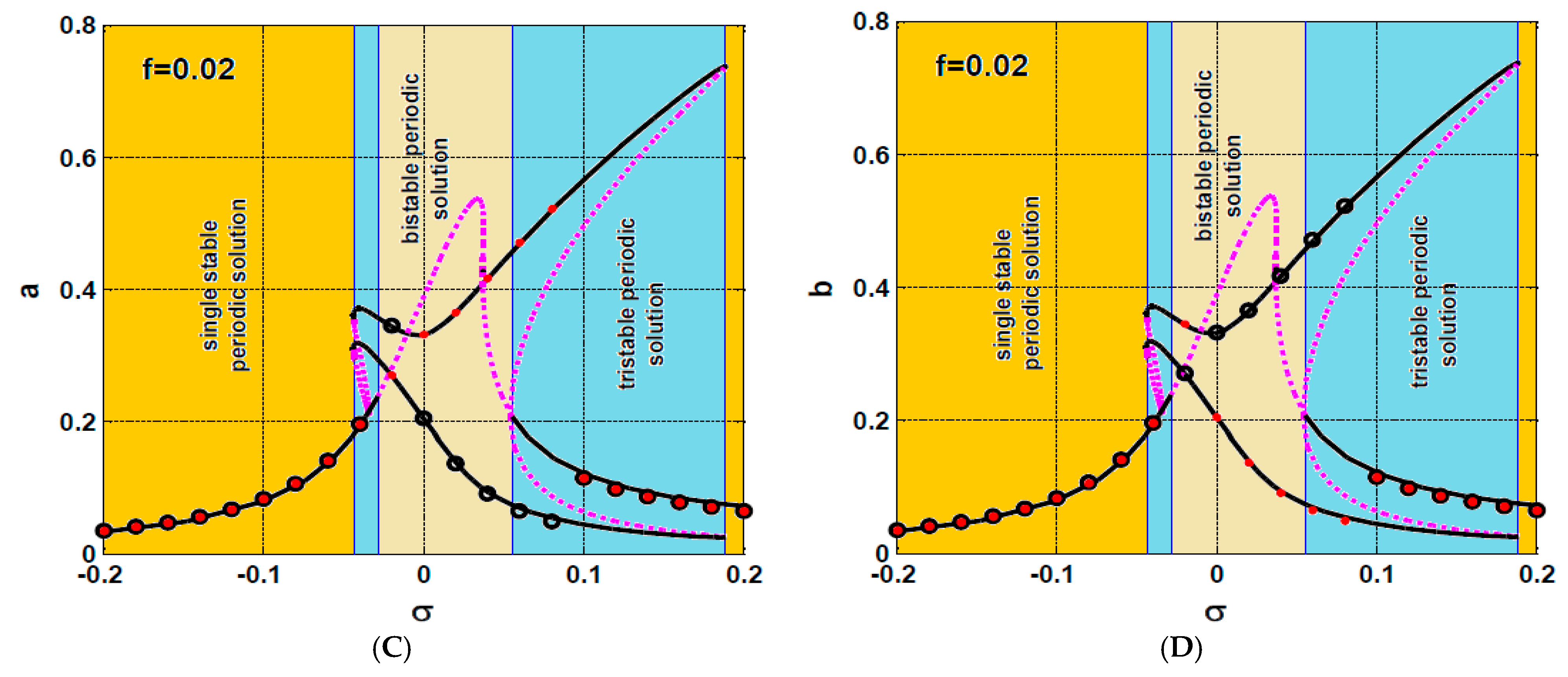
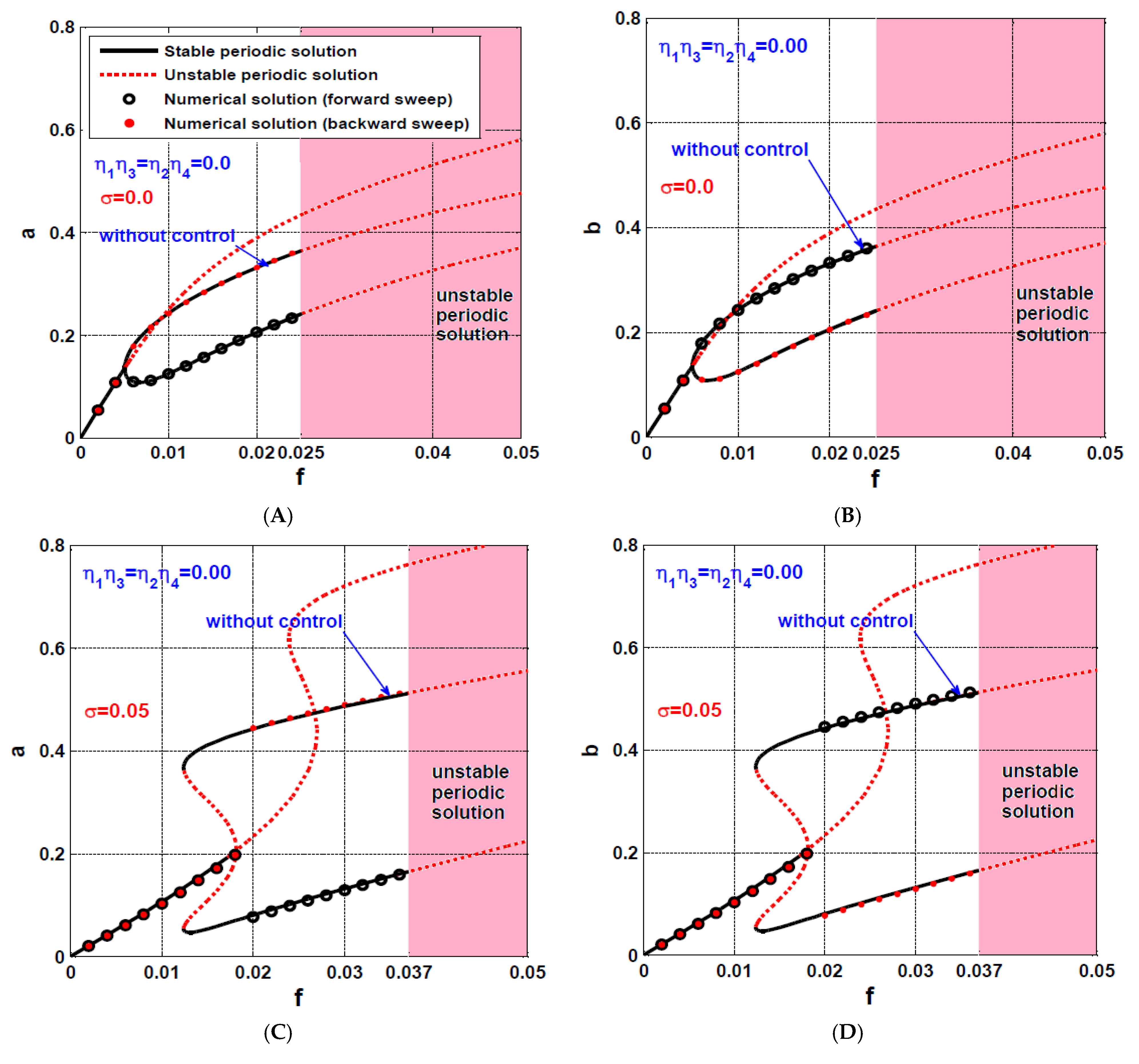
4.1. The Rotor System Dynamics without IRC

The steady-state nonlinear vibration of the rotor system is explored within this section when turning the integral resonant controller off (i.e., when η 1 = η 2 = η 3 = η 4 = λ 1 = λ 2 = 0.0 ), while the proportional gain p = 1.22 and the derivative gain d = 0.005 . Remember from Equation (34) that σ represents the closeness of the rotor angular speed Ω to its natural frequency ω . Accordingly, σ is utilized within this article to describe the system oscillatory behaviors close to the resonance conditions (i.e., when Ω ω ). In Figure 3, the rotor system steady-state vibration amplitudes ( a and b ) are plotted versus σ at two different values of the rotor eccentricity f = 0.01 and 0.02 . Figure 3A,B show that the rotor system exhibits a bistable periodic attractor if 0.018 < σ < 0.033 , otherwise, the rotor responds as a linear system with a single periodic attractor when f = 0.01 . In addition, Figure 3C,D illustrate that the rotor system has a complex σ response curve when increasing the eccentricity to f = 0.02 . Figure 3C,D illustrates that the rotor system can oscillate with one of three oscillations modes, which are: single periodic solutions, bistable periodic solutions, and tri-stable periodic solutions.
To visualize the bifurcation behaviors of the rotor system for a wide range of the eccentricity, f is utilized as the main bifurcation parameter as shown in Figure 4 at two different values of the rotor spinning speed Ω = ω + σ ,   σ = 0.0 ,   0.05 . It is clear from the figure that the rotor system may lose its stability at strong eccentricity beside the three oscillations modes reported in Figure 3. Due to the complex dynamical behaviors of the considered system that are reported in Figure 3 and Figure 4, the integral resonant controller is introduced as a novel control technique to mitigate the nonlinear oscillation and to suppress the motion bifurcations of such system as discussed in Section 4.2.

4.2. The Rotor System Dynamics with IRC

This section is dedicated to exploring the influence of one of the connected integral resonant controllers on the oscillatory behaviors of the rotor system when the other one is turned off. Before investigating the effects of the IRC using the different bifurcation diagrams, let us first examine the derived amplitude-phase equations (i.e., Equations (38)–(41)). It is clear from Equations (38)–(41) that the coupling of the IRC to the rotor system has modified the rotor linear damping coefficient ( μ ) to the equivalent damping coefficients μ x = μ + η 1 η 3 2 ( λ 1 2 + ω 2 ) for the horizontal oscillation mode, and μ y = μ + η 2 η 4 2 ( λ 2 2 + ω 2 ) for the vertical oscillation mode. In addition, the detuning parameter ( σ ) has been modified to σ x = σ + λ 1 η 1 η 3 2 ω ( λ 1 2 + ω 2 ) for the horizontal oscillation mode, and σ y = σ + λ 2 η 2 η 4 2 ω ( λ 2 2 + ω 2 ) for the vertical oscillation mode. Accordingly, the IRC adds the linear damping magnitude η 1 η 3 2 ( λ 1 2 + ω 2 ) to the horizontal oscillation mode and the linear damping magnitude η 2 η 4 2 ( λ 2 2 + ω 2 ) to the vertical oscillation mode. It is worthy to note that μ x is proportional to the product of both the control signal gain ( η 1 ) and feedback signal gain ( η 3 ), and inversely proportional to the square of the internal loop feedback gain ( λ 1 ) of the IRC that is connected to the horizontal oscillation mode. In addition, μ y is proportional to the product of both the control signal gain ( η 2 ) and feedback signal gain ( η 4 ), and inversely proportional to the square of the internal loop feedback gain ( λ 2 ) of the IRC that is connected to the vertical oscillation mode. Moreover, it should be noted that η 1 ,   η 2 ,   η 3 ,   η 4 ,   λ 1 , and λ 2 are the dimensionless forms of the original parameters k 3 ,   k 4 ,   k 5 ,   k 6 ,   ρ 1 , and ρ 2 , respectively. Therefore, we can deduce that the IRC that connected to the horizontal oscillation mode adds linear damping magnitude proportional to the product of the actual feedback and control signal gains ( k 3 k 5 ), while the IRC that is connected to the vertical oscillation mode adds linear damping magnitude proportional to the product of the actual feedback and control signal gains ( k 4 k 6 ) as shown in Figure 2.
For simplicity, let us denote the IRC that is connected to the horizontal oscillation mode as U-IRC and the IRC that is connected to the vertical oscillation mode as V-IRC. Based on the previous discussion, setting η 1 or η 3 or both to be equal to zero means the U-IRC is turned off. Also, setting η 2 or η 4 or both to be equal to zero means the V-IRC is turned off. Accordingly, the influence of the proposed IRC on the response curves of the rotor system has been investigated in two stages of analysis. Firstly, it is considered that the U-IRC is in action, while the V-IRC is deactivated via setting η 2 = 0 or η 4 = 0 or η 2 = η 4 = 0 . Secondly, the effect of both U-IRC and V-IRC on the rotor system is investigated simultaneously as one symmetric IRC.
  • The influence of asymmetric IRC on the rotor system dynamics
The effect of the U-IRC on the rotor system dynamics has been explored within this section considering the V-IRC controller is turned off via setting η 2 = 0 or η 4 = 0 or η 2 = η 4 = 0 . Figure 5 shows the controlled rotor system σ response curve at three different values of the control signal gain η 1 (i.e., η 1 = 0.05 ,   0.2 , and 0.4 ) when η 2 = 0 ,   η 3 = η 4 = 0.2 . It is clear from the figure that the increase of the control signal gain η 1 , decreases the system oscillations in the horizontal direction only, and eliminates the complex bifurcation behaviors of the whole system close to the resonance condition (i.e., when σ close to or equal to zero). The obtained results in Figure 5 can be explained based on the modified linear damping coefficients μ x = μ + η 1 η 3 2 ( λ 1 2 + ω 2 ) and μ y = μ + η 2 η 4 2 ( λ 2 2 + ω 2 ) , where increasing η 1 with letting η 2 = 0 ,   η 3 = η 4 = 0.2 means increasing μ x with fixing μ y = μ . Therefore, the system oscillation at the horizontal direction decreases monotonically with increasing η 1 .
Numerical simulation for the controlled system according to Figure 5 when σ = 0.0 is illustrated in Figure 6 and Figure 7 via solving Equations (12)–(15) using ODE45 at the two different initial conditions x ( 0 ) = x ˙ ( 0 ) = y ( 0 ) = y ˙ ( 0 ) = u ( 0 ) = v ( 0 ) = 0 and x ( 0 ) = 0.2 ,   x ˙ ( 0 ) = y ( 0 ) = y ˙ ( 0 ) = u ( 0 ) = v ( 0 ) = 0 . Figure 6 shows the steady-state time-response and the corresponding orbital motions of the rotor system and the connected IRCs when σ = 0.0 ,   η 1 = 0.05 ,   η 2 = 0 ,   η 3 = η 4 = 0.2 . It is clear from the figure that the rotor system is sensitive to the initial conditions, where the system has two bistable periodic solutions as reported in Figure 5A,B. Moreover, the rotor whirling motion may be forward or backward depending on the initial conditions.
Figure 7 illustrates the time-response and corresponding periodic orbits of the rotor system and IRCs according to Figure 5E,F when σ = 0.0 ,   η 1 = 0.4 ,   η 2 = 0 ,   η 3 = η 4 = 0.2 using the same initial conditions that were used to obtain Figure 6. The figure confirms that the rotor system became insensitive to the initial condition when increasing the control signal gain η 1 to 0.4 , where the rotor exhibits backward whirling motion only regardless of the initial conditions. It is clear from Figure 7 that the system oscillation amplitude at the X direction is about half of the system oscillation amplitude in Y direction that agrees with the system response curve given in Figure 5E,F.
According to Equations (38) and (41), the equivalent linear damping coefficient μ x = μ + η 1 η 3 2 ( λ 1 2 + ω 2 ) is proportional to the product of the control signal gain η 1 and the feedback signal gain η 3 regardless of the magnitude of each one individually. Also, the equivalent linear damping coefficient μ y = μ + η 2 η 4 2 ( λ 2 2 + ω 2 ) is proportional to the product of the control gain η 2 and the feedback signal gain η 4 regardless of the magnitude of each one individually. The influence of product of the control and feedback signal gains of the U-IRC (i.e., η 1 η 3 ) on the rotor system σ response curve when η 2 η 4 = 0.0 is illustrated in Figure 8. The figure shows the system response curves at η 1 η 3 = 0.01 ,   0.04 , and 0.08 . Comparing Figure 8A,B with Figure 5A,B, we can note that the two figures are the same, where the product of η 1 η 3 = 0.01 and η 2 η 4 = 0.0 . Also, Figure 5C,D and Figure 8C,D are identical, where η 1 η 3 = 0.04 and η 2 η 4 = 0.0 . In addition, Figure 5E,F and Figure 8E,F are the same because η 1 η 3 = 0.08 and η 2 η 4 = 0.0 . According to Figure 5 and Figure 8, we can confirm that the coupling of an IRC to any dynamical system can mitigate the system’s nonlinear oscillations via adding a linear damping coefficient that is proportional to the product of the feedback and control signal gains of the coupled controller.
The influence of increasing the eccentricity ( f ) on the rotor system oscillation amplitude when activating the U-IRC such that η 1 η 3 = 0.04 with turning off the V-IRC (i.e., η 2 η 4 = 0.0 ) is illustrated in Figure 9. The figure shows the system f —response curve at two different values of the rotor spinning speed ( Ω = ω + σ ,   σ = 0.0 ,   0.05 ). It is clear from the figure that the rotor system responds as a linear system with a single periodic attractor at the small eccentricity magnitudes ( f ). However, the nonlinear behaviors may dominate the system response when f is increased beyond a critical value. Figure 9A,B show that the system may respond with a single periodic solution as long as f < 0.01199 , but the rotor may respond with one of two stable periodic solutions depending on the initial conditions if 0.01199 < f < 0.02779 . The figure also illustrates that the rotor system can exhibit either a periodic or aperiodic solution depending on the initial conditions if 0.02779 < f < 0.0366 , but the system performs aperiodic oscillations if the eccentricity is increased beyond 0.0366 . Figure 9C,D illustrate the rotor system f response curve when σ = 0.05 . It is clear from the figure the complex dynamics of the rotor system when increasing f from z e r o to 0.05 , where the system responds with a single periodic solution as long as f [ 0 , 0.01245 [ ] 0.01652 ,   0.02058 ] , but the system has bistable periodic solutions as long as f [ 0.01245 ,   0.01652 [ ]   0.02058 ,   0.044 ] . In addition, the rotor system exhibits periodic or aperiodic solution depending on the initial conditions if f > 0.044 .
The stability charts of the 8-pole rotor system are plotted in f η 1 η 3 plane to show the stable and unstable solution regions when σ = 0.0 ,   0.05 as illustrated in Figure 10. It is clear from the figure that the increase of η 1 η 3 , increases the stable solution region which guarantees the stable oscillations of the system at the large magnitude of the rotor eccentricity. Also, the figure confirms that the rotor system has three oscillation modes when activating the U-IRC controller only. These three modes are (1) stable periodic solution only regardless of the initial conditions, (2) stable or unstable periodic solution depending on the initial conditions, and (3) unstable periodic solution only regardless of the initial conditions. To validate the accuracy of the obtained stability chart in Figure 10, numerical simulations for the system equations of motion (i.e., Equations (12)–(15)) are performed as shown in Figure 11, Figure 12 and Figure 13 according to the three points ( p 1 ,   p 2 ,   p 3 ) that marked in Figure 10B. Figure 11 shows the steady-state temporal oscillations of the rotor system and the connected IRCs according to the point p 1 that marked in Figure 10B (i.e., when f = 0.075 , η 1 η 3 = 0.05 ,   η 2 = 0.0 ,   η 4 = 1 ). The figure shows the temporal oscillations and the corresponding Poincaré-map at the initial conditions x ( 0 ) = x ˙ ( 0 ) = y ( 0 ) = y ˙ ( 0 ) = u ( 0 ) = v ( 0 ) = 0 and x ( 0 ) = 0.3 ,   x ˙ ( 0 ) = y ( 0 ) = y ˙ ( 0 ) = u ( 0 ) = v ( 0 ) = 0 . It is clear from Figure 11 that both the system and the controllers oscillate with aperiodic motion regardless of the initial conditions that agree with the point p 1 that marked in Figure 10B. Figure 12 illustrates the temporal oscillations and the corresponding Poincaré-map of both the rotor system and the IRCs according to the point p 2 that showed in Figure 10B (i.e., when f = 0.075 , η 1 η 3 = 0.15 ,   η 2 = 0.0 ,   η 4 = 1 ). It is clear from the figure that the rotor system vibrates with aperiodic motion at zero initial conditions (i.e., x ( 0 ) = x ˙ ( 0 ) = y ( 0 ) = y ˙ ( 0 ) = u ( 0 ) = v ( 0 ) = 0 ), but modifying the initial conditions so that x ( 0 ) = 0.3 ,   x ˙ ( 0 ) = y ( 0 ) = y ˙ ( 0 ) = u ( 0 ) = v ( 0 ) = 0 , has forced the rotor system to oscillate periodically. Accordingly, Figure 12 confirms that the rotor system may respond with a periodic or aperiodic motion depending on the initial conditions that agree with the point p 2 that marked in Figure 10B. The nonlinear oscillations of the rotor system and the connected controller are simulated as shown in Figure 13 according to the point p 3 that illustrated in Figure 10B (i.e., when f = 0.075 , η 1 η 3 = 0.25 ,   η 2 = 0.0 ,   η 4 = 1 ). The figure is obtained using the two different initial conditions that are used to obtain Figure 11 and Figure 12. It is clear from Figure 13 that the system is insensitive to the initial conditions, where the system responds periodically with the same oscillation amplitude regardless of the initial conditions that agree with the point p 3 that is marked in Figure 10B.
b.
The influence of symmetric IRC on the rotor system dynamics
The dynamical behavior of the rotor system when activating both the U-IRC and V-IRC controllers simultaneously is discussed in this section. Figure 14 shows the steady-state oscillation amplitudes of the rotor system ( a   &   b ) versus the parameter σ at three different values of the product of the control and feedback gains (i.e., when η 1 η 3 = η 2 η 4 = 0.01 ,   0.04 ,   0.08 ). It is clear from the figure that the increase of η 1 η 3 = η 2 η 4 , increases the system equivalent linear damping coefficients μ x and μ y as discussed before, which ultimately decreases the system oscillation amplitudes and eliminates the motion bifurcations as illustrated in Figure 14E,F. Comparing Figure 14 with Figure 8, it is clear from Figure 8E,F that the rotor system responds as a nonlinear system with a bistable periodic attractor at a specific range of the rotor spinning speed when η 1 η 3 = 0.08   &   η 2 η 4 = 0.0 , while Figure 14E,F show that the system responds as a linear one with a single periodic attractor regardless of the rotor spinning speed when η 1 η 3 = η 2 η 4 = 0.08 . Accordingly, we can deduce that the dynamical behavior of the rotor system when activating one of the IRCs is completely different than the system dynamic when both the U-IRC and V-IRC are activated simultaneously. It is clear from Figure 14 that the worst resonance occurs at σ = 0.0 , therefore η 1 η 3 = η 2 η 4 are used as a bifurcation parameter to explore the influence of increasing η 1 η 3 = η 2 η 4 on the system oscillation amplitudes when σ = 0.0 as illustrated in Figure 15. It is clear from the figure that the system oscillations amplitudes are a monotonic decreasing function of η 1 η 3 = η 2 η 4 . In addition, the figure confirms the system bistable oscillation amplitudes have been merged into a single periodic attractor when η 1 η 3 = η 2 η 4 exceeded a specific value.
It has been concluded before that the coupling of the IRCs to the rotor system modified the rotor linear damping coefficient ( μ ) to the equivalent damping coefficients μ x = μ + η 1 η 3 2 ( λ 1 2 + ω 2 ) and μ y = μ + η 2 η 4 2 ( λ 2 2 + ω 2 ) . In addition, the detuning parameter ( σ ) has been modified to σ x = σ + λ 1 η 1 η 3 2 ω ( λ 1 2 + ω 2 ) and σ y = σ + λ 2 η 2 η 4 2 ω ( λ 2 2 + ω 2 ) . Accordingly, the influence of internal loop feedback gains ( λ 1 and λ 2 ) of the IRCs on the oscillation amplitudes ( a   &   b ) is illustrated in Figure 16, where Figure 16A,B show the rotor system oscillation amplitudes at λ 1 = λ 2 = 0.1 ,   1.0 when η 1 η 3 = η 2 η 4 = 0.08 . It is clear from Figure 16A,B that the rotor system vibration amplitudes ( a and b ) when λ 1 = λ 2 = 0.1 is smaller than its oscillation amplitudes when λ 1 = λ 2 = 1.0 . It is worthy to mention that the obtained results in Figure 16A,B agree with the derived equations of the equivalent linear damping coefficients μ x and μ y , where μ x and μ y inversely proportional to 2 λ 1 2 and to 2 λ 2 2 , respectively. Moreover, Figure 16A,B indicate that internal loop feedback gains ( λ 1 and λ 2 ) play an important role in shifting the system σ response curve to the right or the left via modifying the detuning parameter σ to σ x = σ + λ 1 η 1 η 3 2 ω ( λ 1 2 + ω 2 ) and σ y = σ + λ 2 η 2 η 4 2 ω ( λ 2 2 + ω 2 ) . Figure 16C,D shows the rotor system oscillation amplitude at η 1 η 3 = η 2 η 4 = 0.08 when the internal loop feedback gains are increased to λ 1 = λ 2 = 2.0 . Comparing Figure 16C,D with Figure 16A,B, we can confirm that the increase of the internal loop feedback gains from λ 1 = λ 2 = 1.0 to λ 1 = λ 2 = 2.0 , has decreased equivalent damping coefficients μ x and μ y , which ultimately forced the rotor system to respond as a nonlinear one with high vibration amplitudes.
The f response curve of the rotor system when η 1 η 3 = η 2 η 4 = 0.08 are illustrated in Figure 17 at two different values of the rotor spinning speed Ω = ω + σ ,   σ = 0.0 ,   0.05 . It is clear from Figure 17 that the controlled rotor system will respond with periodic motion as long as 0.0 f 0.05 . However, the system may respond as a linear system with a single periodic attractor or as a nonlinear one with a bistable periodic attractor depending on the eccentricity magnitude. Comparing Figure 17 with Figure 4, we can confirm that the activation of both the U-IRC and V-IRC simultaneously has eliminated the unstable oscillation of the uncontrolled rotor system that showed in Figure 4. In addition, the four oscillation modes that are noticed in Figure 9 when activating the U-IRC only, have been reduced to two desirable oscillation modes only as illustrated in Figure 17, which are single and bistable periodic motion.
A full picture for the stability boundary in f η 1 η 3 = η 2 η 4 is visualized as shown in Figure 18 when σ = 0.0 and 0.05 . It is clear from the figure the increase of the controller gain ( η 1 η 3 = η 2 η 4 ), stabilizes the system motion for a wide range of the rotor eccentricity, where the width of the stable solution regions along the f axis is increased exponentially as a function of the control gain η 1 η 3 = η 2 η 4 . Comparing Figure 18 with Figure 10, one can deduce that the controlled system has simple bifurcation behaviors when activating both the U-IRC and V-IRC simultaneously. In addition, the system can oscillate periodically without losing its stability for a wide range of the excitation force f .
To validate the accuracy of the obtained stability charts in Figure 18, numerical simulations for the system temporal equations (i.e., Equations (12)–(15)) are illustrated in Figure 19 and Figure 20 according to the points p 1 and p 2 that illustrated in Figure 18A, respectively. The temporal oscillation, frequency spectrum, and the corresponding Poincaré-map of the controlled rotor system are illustrated in Figure 19 according to the points p 1 ( f ,   η 1 η 3 = η 2 η 4 ) = ( 0.15 ,   0.1 ) that is marked in Figure 18A within the unstable solution region. It is clear from Figure 19 that the rotor system exhibits chaotic oscillations (i.e., aperiodic motion) as predicted in the stability chart given in Figure 18A. In addition, Figure 20 simulates the temporal oscillations, frequency spectrum, and the corresponding Poincaré-map of the rotor system according to the points p 2 ( f ,   η 1 η 3 = η 2 η 4 ) = ( 0.15 ,   0.25 ) illustrated in Figure 18A within the stable solution region. By examining Figure 20, one can conclude that the rotor system performs a stable periodic motion that agrees with the stability chart given in Figure 18A with excellent accuracy.
Finally, the controlled system stability chart in σ η 1 η 3 = η 2 η 4 has been established as shown in Figure 21 at three different magnitudes of the eccentricity f (i.e., f = 0.05 ,   0.1 , and 0.15 ). It is clear from the figure that the unstable solutions area lies close to the primary resonance (i.e., close to σ = 0.0 ). In addition. The figure shows that the increase of the excitation force f , increases the unstable solution region. However, one can avoid the instability of the rotor system even at the large eccentricity (i.e., f = 0.15 ) if the control gains are adjusted so that η 1 η 3 = η 2 η 4 0.15 regardless of the rotor spinning speed Ω = ω + σ (See Figure 21C). Numerical validations for the accuracy of the obtained stability charts that are given in Figure 21 have been illustrated in Figure 22 and Figure 23. The nonlinear vibrations of the rotor system according to the point p 1 ( σ ,   η 1 η 3 = η 2 η 4 ) = p 1 ( 0 ,   0.1 ) that lies within the unstable solution region in Figure 21B, have been simulated numerically as shown in Figure 22 via solving Equations (14)–(17) using ODE45. By exploring Figure 22, we can find that the rotor system performs an unstable quasiperiodic motion that agrees with the point p 1 . On the other hand, the temporal oscillations of the considered system according to the point p 2 ( σ ,   η 1 η 3 = η 2 η 4 ) = p 2 ( 0 ,   0.15 ) that lies within the stable solution region in Figure 21B, have been illustrated in Figure 23, where the system has responded with periodic oscillation as expected from Figure 21B.

5. Case Study

Within this section, a practical case study for the 8-pole rotor system with the proposed control method (i.e., PD+IRC controller) has been investigated to show how to simulate the dynamics of a physical system based on the obtained dimensionless results given in Section 4. Consider the dimensionless system parameters that are used to obtain Figure 23 and corresponding physical parameters of the eight-pole system given in Table 1 [41,42]. The actual temporal oscillations (i.e., x ( t ) = s 0 x * ( t ) & y ( t ) = s 0 y * ( t ) ) and the corresponding actual control currents ( i x ( t ) = k 1 x ( t ) + k 2 x ˙ ( t ) + k 3 u ( t )   &   i y ( t ) = k 1 y ( t ) + k 2 y ˙ ( t ) + k 4 v ( t ) of the rotor system are simulated in Figure 24, where the actual control current can be obtained based on Equation (6) as follows: i x ( t ) = k 1 s 0 x * ( t ) + k 2 s 0 ω n x ˙ * ( t ) + k 3 s 0 u * ( t ) and i y ( t ) = k 1 s 0 y * ( t ) + k 2 s 0 ω n y ˙ * ( t ) + k 4 s 0 v ( t ) .
Figure 24 shows the actual temporal oscillations of the 8-pole rotor system in meter at X and Y directions, and the corresponding actual control currents in ampere in each electromagnetic pole according to the system physical parameters given in Table 1. It is clear from Figure 24A,B that the rotor lateral oscillations are always smaller than the air gap along the time axis, which confirm the rotational motions of the shaft without any contact with the legs of the electromagnetic poles. Also, Figure 24C,D show that the maximum instantaneous control currents in each pole do not exceed two amperes, which confirm the feasibility of the applied control algorithm in mitigating the rotor lateral oscillation with small control currents.

6. Conclusions

The nonlinear vibrations control of the 8-pole rotor system has been tackled within this article. The integral resonant controller (IRC) has been proposed to control the system lateral vibrations for the first time. The U-IRC and V-IRC controllers have been coupled to the horizontal and vertical oscillation modes of the considered system, respectively. The whole system equations of motion are derived as two second-order nonlinear differential equations (i.e., rotor system) coupled to two first-order linear differential equations (i.e., IRC controllers). Then, the asymptotic analysis is applied to obtain an approximate solution for the derived nonlinear mathematical model. The different bifurcation diagrams have been plotted and the sensitivity analysis for all controller parameters has been explored. In addition, many stability charts in the two-dimensional space have been established to investigate the stability margins of the different control parameters. Moreover, numerical validations for the different response curves have been performed. According to the above discussions, the following important remarks can be summarized:
  • The coupling of the U-IRC to the horizontal oscillation mode of the rotor system has modified the system linear damping coefficient μ to μ x = μ + η 1   η 3 2 ( λ 1 2 + ω 2 ) .
  • The coupling of the V-IRC to the vertical oscillation mode of the rotor system has modified the system linear damping coefficient μ to μ y = μ + η 2   η 4 2 ( λ 2 2 + ω 2 ) .
  • According to the concluded points (1) and (2), the vibration suppression efficiency of the IRC relies on adjusting the linear damping coefficient for the targeted system via designing the optimum values of the control gains ( η 1 ,   η 2 ), feedback gains ( η 3 ,   η 4 ), and internal feedback gains ( λ 1 ,   λ 2 ).
  • The coupling of an IRC to a nonlinear oscillatory system is resulting in modifying its linear damping coefficient, where the equivalent linear damping of the controlled system is proportional to the product of the control and feedback gains of the IRC, and inversely proportional to the square of internal loop feedback gain.
  • The optimum vibration suppression efficiency of the IRC controller could be achieved via designing its control and feedback gains so that their product is at the maximum possible value, as well as its internal feedback gain should be at the smallest possible value.
  • The proper selection of the IRC control parameters can eliminate the catastrophic static bifurcation behaviors of the rotor system and force it to oscillate with negligible vibration amplitudes.

Author Contributions

Conceptualization, N.A.S. and J.A.; Formal analysis, N.A.S.; Funding acquisition, M.S.M. and J.A.; Investigation, N.A.S., S.K.E. and J.A.; Methodology, N.A.S. and J.A.; Project administration, N.A.S., M.S.M. and J.A.; Resources, N.A.S., M.S.M. and S.K.E.; Software, N.A.S. and S.K.E.; Supervision, J.A.; Validation, N.A.S., S.K.E. and J.A.; Visualization, N.A.S. and S.K.E.; Writing—original draft, N.A.S.; Writing—review & editing, N.A.S., M.S.M., S.K.E. and J.A. All authors have read and agreed to the published version of the manuscript.

Funding

This research was funded by Researchers Supporting Project, Taif University, Taif, Saudi Arabia under grant number TURSP-2020/160. This work was also supported by the National Science Centre, Poland under grant number OPUS 14 No. 2017/27/B/ST8/01330.

Institutional Review Board Statement

Not applicable.

Informed Consent Statement

Not applicable.

Data Availability Statement

Not applicable.

Acknowledgments

The authors would like to thank Taif University, where this work was supported by the Taif University Researchers Supporting Project number (TURSP-2020/160), Taif, Saudi Arabia.

Conflicts of Interest

The authors declared no potential conflicts of interest with respect to the research, authorships, and/or publication of this article.

Abbreviations

x , x ˙ , x ¨ Displacement, velocity, and acceleration of the rotor system in X direction
y , y ˙ , y ¨ Displacement, velocity, and acceleration of the rotor system in Y direction
u , u   ˙ Displacement and velocity of the integral resonant controller that connected to the horizontal oscillation mode of the rotor system
v , v ˙ Displacement and velocity of the integral resonant controller that connected to the vertical oscillation mode of the rotor system
μ Linear damping coefficient of the rotor system
ω Linear natural frequency of the rotor system
Ω Spinning speed of the rotor system
f Rotor system eccentricity
η 1 , η 2 Control gains of the integral resonant controllers
η 3 , η 4 Feedback gains of the integral resonant controllers
λ 1 , λ 2 Internal loop feedback gains of the integral resonant controllers
p Proportional control gain
d Derivative control gain
α j , j = 1 , , 7 Cubic nonlinearity coupling coefficients due to the proportional-derivative controller
β j , j = 1 , , 7 Cubic nonlinearity coupling coefficients due to the integral resonant controller in X direction
γ j , j = 1 , , 7 Cubic nonlinearity coupling coefficients due to the integral resonant controller in Y direction
σ The   main   bifurcation   parameter ,   where   σ = Ω ω
a , b Steady-state oscillation amplitudes of the rotor system in X and Y directions
φ 1 , φ 2 Steady-state phase angles of the rotor system in X and Y directions

Appendix A

F X C = Δ s 0 3 [ ( 8 I 0 2 8 I 0 s 0 k 1 cos ( α ) ) x + ( 8 I 0 s 0 k 2 cos ( α ) ) x ˙ + ( 16 I 0 2 cos 4 ( α ) + 16 I 0 2 sin 4 ( α ) + 8 s 0 2 k 1 2 cos 2 ( α ) 24 I 0 s 0 k 1 cos 3 ( α ) ) x 3 + ( 8 s 0 2 k 1 2 sin 2 ( α ) + 96 I 0 2 cos 2 ( α ) sin 2 ( α ) 72 I 0 s 0 k 1 cos ( α ) sin 2 ( α ) ) x y 2 + ( 16 k 1 k 2 s 0 2 cos 2 ( α ) 24 I 0 k 2 s 0 cos 3 ( α ) ) x 2 x ˙ + ( 8 k 2 2 s 0 2 cos 2 ( α ) ) x x ˙ 2 + ( 24 I 0 k 2 s 0 cos ( α ) sin 2 ( α ) ) x ˙ y 2 + ( 8 k 2 2 s 0 2 sin 2 ( α ) ) x y ˙ 2 + ( 16 k 1 k 2 s 0 2 sin 2 ( α ) 48 I 0 k 2 s 0 cos ( α ) sin 2 ( α ) ) x y y ˙ + ( 16 k 1 k 3 s 0 2 cos 2 ( α ) 24 I 0 k 3 s 0 cos 3 ( α ) ) x 2 u + ( 16 k 2 k 3 s 0 2 cos 2 ( α ) ) x x ˙ u + ( 8 k 3 2 s 0 2 cos 2 ( α ) ) x u 2 + ( 16 k 1 k 4 s 0 2 sin 2 ( α ) 48 I 0 k 4 s 0 cos ( α ) sin 2 ( α ) ) x y v + ( 8 k 4 2 s 0 2 sin 2 ( α ) ) x v 2 + ( 16 k 2 k 4 s 0 2 sin 2 ( α ) ) x y ˙ v ( 24 I 0 k 3 s 0 cos ( α ) sin 2 ( α ) ) y 2 u ( 8 I 0 k 3 s 0 cos ( α ) ) u ]
F Y C = Δ s 0 3 [ ( 8 I 0 2 8 I 0 s 0 k 1 cos ( α ) ) y + ( 8 I 0 s 0 k 2 cos ( α ) ) y ˙ + ( 16 I 0 2 cos 4 ( α ) + 16 I 0 2 sin 4 ( α ) + 8 s 0 2 k 1 2 cos 2 ( α ) 24 I 0 s 0 k 1 cos 3 ( α ) ) y 3 + ( 8 s 0 2 k 1 2 sin 2 ( α ) + 96 I 0 2 cos 2 ( α ) sin 2 ( α ) 72 I 0 s 0 k 1 cos ( α ) sin 2 ( α ) ) y x 2 + ( 16 k 1 k 2 s 0 2 cos 2 ( α ) 24 I 0 k 2 s 0 cos 3 ( α ) ) y 2 y ˙ + ( 8 k 2 2 s 0 2 cos 2 ( α ) ) y y ˙ 2 + ( 24 I 0 k 2 s 0 cos ( α ) sin 2 ( α ) ) y ˙ x 2 + ( 8 k 2 2 s 0 2 sin 2 ( α ) ) x y ˙ 2 + ( 16 k 1 k 2 s 0 2 sin 2 ( α ) 48 I 0 k 2 s 0 cos ( α ) sin 2 ( α ) ) y x x ˙ + ( 16 k 1 k 4 s 0 2 cos 2 ( α ) 24 I 0 k 4 s 0 cos 3 ( α ) ) y 2 v + ( 16 k 2 k 4 s 0 2 cos 2 ( α ) ) y y ˙ v + ( 8 k 4 2 s 0 2 cos 2 ( α ) ) y v 2 + ( 16 k 1 k 3 s 0 2 sin 2 ( α ) 48 I 0 k 3 s 0 cos ( α ) sin 2 ( α ) ) y x u + ( 8 k 3 2 s 0 2 sin 2 ( α ) ) y u 2 + ( 16 k 2 k 3 s 0 2 sin 2 ( α ) ) y x ˙ u ( 24 I 0 k 4 s 0 cos ( α ) sin 2 ( α ) ) x 2 v ( 8 I 0 k 4 s 0 cos ( α ) ) v ]

Appendix B

μ = 4 d cos ( α ) , ω = 8 p cos ( α ) 8 ,
α 1 = 16 cos 4 ( α ) + 16 sin 4 ( α ) + 8 p 2 cos 2 ( α ) 24 p cos 3 ( α ) ,
α 2 = 8 p 2 sin 2 ( α ) + 96 cos 2 ( α ) sin 2 ( α ) 72 p cos ( α ) sin 2 ( α ) ,
α 3 = 16 p d cos 2 ( α ) 24 d cos 3 ( α ) , α 4 = 24 d cos ( α ) sin 2 ( α ) ,
α 4 = 24 d cos ( α ) sin 2 ( α ) , α 5 = 8 d 2 sin 2 ( α ) ,
α 6 = 8 d 2 cos 2 ( α ) , α 7 = 16 p d sin 2 ( α ) 48 d cos ( α ) sin 2 ( α ) ,
β 1 = 2 p η 1 cos ( α ) + 3 η 1 cos 2 ( α ) , β 2 = 2 d η 1 cos ( α ) ,
β 3 = 1 8 η 1 2 , β 4 = 2 p η 2 tan ( α ) sin ( α ) + 6 η 2 sin 2 ( α ) ,
β 5 = 1 8 η 2 2 tan 2 ( α ) , β 6 = 2 d η 2 tan ( α ) sin ( α ) ,
β 7 = 3 η 1 sin 2 ( α ) , γ 1 = 2 p η 2 cos ( α ) + 3 η 2 cos 2 ( α ) ,
γ 2 = 2 d η 2 cos ( α ) , γ 3 = 1 8 η 2 2 ,
γ 4 = 2 p η 1 tan ( α ) sin ( α ) + 6 η 1 sin 2 ( α ) , γ 5 = 1 8 η 1 2 tan 2 ( α )
γ 6 = 2 d η 1 tan ( α ) sin ( α ) , γ 7 = 3 η 2 sin 2 ( α ) ,

Appendix C

G 1 a 1 = ( μ + η 3 η 1 2 ( λ 1 2 + ω 2 ) ) + 3 8 ( α 3 2 β 1 η 3 λ 1 2 + ω 2 2 β 3 η 3 2 λ 1 ( λ 1 2 + ω 2 ) 2 ) a 0 2 + 1 8 ( 2 α 4 β 4 η 4 λ 2 2 + ω 2 β 6 η 4 λ 2 λ 2 2 + ω 2 2 β 7 η 3 λ 1 2 + ω 2 ) b 0 2 + 1 8 ( α 4 + α 7 β 4 η 4 λ 2 2 + ω 2 + 2 β 5 η 4 2 λ 2 ( λ 2 2 + ω 2 ) 2 + β 6 η 4 λ 2 λ 2 2 + ω 2 ) b 0 2 cos ( 2 φ 20 2 φ 10 ) 1 8 ( α 2 ω α 5 ω + β 4 η 4 λ 2 ω ( λ 2 2 + ω 2 ) + β 5 η 4 2 ( λ 2 2 ω 2 ) ω ( λ 2 2 + ω 2 ) 2 β 6 η 4 ω λ 2 2 + ω 2 ) b 0 2 sin ( 2 φ 20 2 φ 10 ) ,
G 1 b 1 = 1 4 ( 2 α 4 β 4 η 4 λ 2 2 + ω 2 β 6 η 4 λ 2 λ 2 2 + ω 2 2 β 7 η 3 λ 1 2 + ω 2 ) a 0 b 0 + 1 4 ( α 4 + α 7 β 4 η 4 λ 2 2 + ω 2 + 2 β 5 η 4 2 λ 2 ( λ 2 2 + ω 2 ) 2 + β 6 η 4 λ 2 λ 2 2 + ω 2 ) a 0 b 0 cos ( 2 φ 20 2 φ 10 ) 1 4 ( α 2 ω α 5 ω + β 4 η 4 λ 2 ω ( λ 2 2 + ω 2 ) + β 5 η 4 2 ( λ 2 2 ω 2 ) ω ( λ 2 2 + ω 2 ) 2 β 6 η 4 ω λ 2 2 + ω 2 ) a 0 b 0 sin ( 2 φ 20 2 φ 10 ) ,
G 1 φ 11 = 1 4 ( α 4 + α 7 β 4 η 4 λ 2 2 + ω 2 + 2 β 5 η 4 2 λ 2 ( λ 2 2 + ω 2 ) 2 + β 6 η 4 λ 2 λ 2 2 + ω 2 ) a 0 b 0 2 sin ( 2 φ 20 2 φ 10 ) + 1 4 ( α 2 ω α 5 ω + β 4 η 4 λ 2 ω ( λ 2 2 + ω 2 ) + β 5 η 4 2 ( λ 2 2 ω 2 ) ω ( λ 2 2 + ω 2 ) 2 β 6 η 4 ω λ 2 2 + ω 2 ) a 0 b 0 2 cos ( 2 φ 20 2 φ 10 ) + f 2 ω ( ω + σ ) 2 cos ( φ 10 ) ,
G 1 φ 21 = 1 4 ( α 4 + α 7 β 4 η 4 λ 2 2 + ω 2 + 2 β 5 η 4 2 λ 2 ( λ 2 2 + ω 2 ) 2 + β 6 η 4 λ 2 λ 2 2 + ω 2 ) a 0 b 0 2 sin ( 2 φ 2 2 φ 1 ) 1 4 ( α 2 ω α 5 ω + β 4 η 4 λ 2 ω ( λ 2 2 + ω 2 ) + β 5 η 4 2 ( λ 2 2 ω 2 ) ω ( λ 2 2 + ω 2 ) 2 β 6 η 4 ω λ 2 2 + ω 2 ) a 0 b 0 2 cos ( 2 φ 2 2 φ 1 ) ,
G 2 a 1 = 1 4 ( 2 α 4 γ 4 η 3 λ 1 2 + ω 2 γ 6 η 3 λ 1 λ 1 2 + ω 2 2 γ 7 η 4 λ 2 2 + ω 2 ) a 0 b 0 + 1 4 ( α 4 + α 7 γ 4 η 3 λ 1 2 + ω 2 2 γ 5 η 3 2 λ 1 ( λ 1 2 + ω 2 ) 2 + γ 6 η 3 λ 1 λ 1 2 + ω 2 ) a 0 b 0 cos ( 2 φ 20 2 φ 10 ) + 1 4 ( α 2 ω α 5 ω + γ 4 η 3 λ 1 ω ( λ 1 2 + ω 2 ) + γ 5 η 3 2 ( λ 1 2 ω 2 ) ω ( λ 1 2 + ω 2 ) 2 + γ 6 η 3 ω λ 1 2 + ω 2 ) a 0 b 0 sin ( 2 φ 20 2 φ 10 ) ,
G 2 b 1 = ( μ + η 2 η 4 2 ( λ 2 2 + ω 2 ) ) + 3 8 ( α 3 2 γ 1 η 4 λ 2 2 + ω 2 2 γ 3 η 4 2 λ 2 ( λ 2 2 + ω 2 ) 2 ) b 0 2 + 1 8 ( 2 α 4 γ 4 η 3 λ 1 2 + ω 2 γ 6 η 3 λ 1 λ 1 2 + ω 2 2 γ 7 η 4 λ 2 2 + ω 2 ) a 0 2 + 1 8 ( α 4 + α 7 γ 4 η 3 λ 1 2 + ω 2 2 γ 5 η 3 2 λ 1 ( λ 1 2 + ω 2 ) 2 + γ 6 η 3 λ 1 λ 1 2 + ω 2 ) a 0 2 cos ( 2 φ 20 2 φ 10 ) + 1 8 ( α 2 ω α 5 ω + γ 4 η 3 λ 1 ω ( λ 1 2 + ω 2 ) + γ 5 η 3 2 ( λ 1 2 ω 2 ) ω ( λ 1 2 + ω 2 ) 2 + γ 6 η 3 ω λ 1 2 + ω 2 ) a 0 2 sin ( 2 φ 20 2 φ 10 ) ,
G 2 φ 11 = 1 4 ( α 4 + α 7 γ 4 η 3 λ 1 2 + ω 2 2 γ 5 η 3 2 λ 1 ( λ 1 2 + ω 2 ) 2 + γ 6 η 3 λ 1 λ 1 2 + ω 2 ) a 0 2 b 0 sin ( 2 φ 20 2 φ 10 ) 1 4 ( α 2 ω α 5 ω + γ 4 η 3 λ 1 ω ( λ 1 2 + ω 2 ) + γ 5 η 3 2 ( λ 1 2 ω 2 ) ω ( λ 1 2 + ω 2 ) 2 + γ 6 η 3 ω λ 1 2 + ω 2 ) a 0 2 b 0 cos ( 2 φ 20 2 φ 10 )
G 2 φ 21 = 1 4 ( α 4 + α 7 γ 4 η 3 λ 1 2 + ω 2 2 γ 5 η 3 2 λ 1 ( λ 1 2 + ω 2 ) 2 + γ 6 η 3 λ 1 λ 1 2 + ω 2 ) a 0 2 b 0 sin ( 2 φ 20 2 φ 10 ) + 1 4 ( α 2 ω α 5 ω + γ 4 η 3 λ 1 ω ( λ 1 2 + ω 2 ) + γ 5 η 3 2 ( λ 1 2 ω 2 ) ω ( λ 1 2 + ω 2 ) 2 + γ 6 η 3 ω λ 1 2 + ω 2 ) ) a 0 2 b 0 cos ( 2 φ 20 2 φ 10 ) + f 2 ω ( ω + σ ) 2 sin ( φ 2 ) ,
G 3 a 1 = 1 4 ω ( 3 α 1 + α 6 ω 2 + 2 β 1 η 3 λ 1 λ 1 2 + ω 2 + β 3 η 3 2 ( λ 1 2 ω 2 ) ( λ 1 2 + ω 2 ) 2 ) a 0 f 2 a 0 2 ω ( ω + σ ) 2 cos ( φ 10 ) ,
G 3 b 1 = 1 4 ω ( 2 α 2 + 2 α 5 ω 2 + β 4 η 4 λ 2 λ 2 2 + ω 2 β 6 η 4 ω 2 λ 2 2 + ω 2 + 2 β 7 η 3 λ 1 λ 1 2 + ω 2 ) b 0 + 1 4 ω ( α 2 α 5 ω 2 + β 4 η 4 λ 2 λ 2 2 + ω 2 + β 5 η 4 2 ( λ 2 2 ω 2 ) ( λ 2 2 + ω 2 ) 2 + β 6 η 4 ω 2 λ 2 2 + ω 2 ) b 0 cos ( 2 φ 20 2 φ 10 ) + 1 4 ( α 4 + α 7 β 4 η 4 λ 2 2 + ω 2 2 β 5 η 4 2 λ 2 ( λ 2 2 + ω 2 ) 2 + β 6 η 4 λ 2 λ 2 2 + ω 2 ) b 0 sin ( 2 φ 20 2 φ 10 ) ,
G 3 φ 11 = 1 4 ω ( α 2 α 5 ω 2 + β 4 η 4 λ 2 λ 2 2 + ω 2 + β 5 η 4 2 ( λ 2 2 ω 2 ) ( λ 2 2 + ω 2 ) 2 + β 6 η 4 ω 2 λ 2 2 + ω 2 ) b 0 2 sin ( 2 φ 20 2 φ 10 ) 1 4 ( α 4 + α 7 β 4 η 4 λ 2 2 + ω 2 2 β 5 η 4 2 λ 2 ( λ 2 2 + ω 2 ) 2 + β 6 η 4 λ 2 λ 2 2 + ω 2 ) b 0 2 cos ( 2 φ 20 2 φ 10 ) f 2 a 0 ω ( ω + σ ) 2 sin ( φ 10 ) ,
G 3 φ 21 = 1 4 ω ( α 2 α 5 ω 2 + β 4 η 4 λ 2 λ 2 2 + ω 2 + β 5 η 4 2 ( λ 2 2 ω 2 ) ( λ 2 2 + ω 2 ) 2 + β 6 η 4 ω 2 λ 2 2 + ω 2 ) b 0 2 sin ( 2 φ 20 2 φ 10 ) + 1 4 ( α 4 + α 7 β 4 η 4 λ 2 2 + ω 2 2 β 5 η 4 2 λ 2 ( λ 2 2 + ω 2 ) 2 + β 6 η 4 λ 2 λ 2 2 + ω 2 ) b 0 2 cos ( 2 φ 20 2 φ 10 ) ,
G 4 a 1 = 1 4 ω ( 2 α 2 + 2 α 5 ω 2 + γ 4 η 3 λ 1 λ 1 2 + ω 2 γ 6 η 3 ω 2 λ 1 2 + ω 2 + 2 γ 7 η 4 λ 2 λ 2 2 + ω 2 ) a 0 + 1 4 ω ( α 2 α 5 ω 2 + γ 4 η 3 λ 1 λ 1 2 + ω 2 + γ 5 η 3 2 ( λ 1 2 ω 2 ) ( λ 1 2 + ω 2 ) 2 + γ 6 η 3 ω 2 λ 1 2 + ω 2 ) a 0 cos ( 2 φ 20 2 φ 10 ) 1 4 ( α 4 + α 7 + γ 4 η 3 λ 1 2 + ω 2 2 γ 5 η 3 2 λ 1 ( λ 1 2 + ω 2 ) 2 γ 6 η 3 λ 1 λ 1 2 + ω 2 ) a 0 sin ( 2 φ 20 2 φ 10 ) ,
G 4 b 1 = 1 4 ω ( 3 α 1 + α 6 ω 2 + 2 γ 1 η 4 λ 2 λ 2 2 + ω 2 + γ 3 η 4 2 ( λ 2 2 ω 2 ) ( λ 2 2 + ω 2 ) 2 ) b 0 f 2 b 0 2 ω ( ω + σ ) 2 sin ( φ 20 ) ,
G 4 φ 11 = 1 4 ω ( α 2 α 5 ω 2 + γ 4 η 3 λ 1 λ 1 2 + ω 2 + γ 5 η 3 2 ( λ 1 2 ω 2 ) ( λ 1 2 + ω 2 ) 2 + γ 6 η 3 ω 2 λ 1 2 + ω 2 ) a 0 2 sin ( 2 φ 20 2 φ 10 ) + 1 4 ( α 4 + α 7 + γ 4 η 3 λ 1 2 + ω 2 2 γ 5 η 3 2 λ 1 ( λ 1 2 + ω 2 ) 2 γ 6 η 3 λ 1 λ 1 2 + ω 2 ) a 0 2 cos ( 2 φ 20 2 φ 10 ) ,
G 4 φ 21 = 1 4 ω ( α 2 α 5 ω 2 + γ 4 η 3 λ 1 λ 1 2 + ω 2 + γ 5 η 3 2 ( λ 1 2 ω 2 ) ( λ 1 2 + ω 2 ) 2 + γ 6 η 3 ω 2 λ 1 2 + ω 2 ) a 0 2 sin ( 2 φ 20 2 φ 10 ) 1 4 ( α 4 + α 7 + γ 4 η 3 λ 1 2 + ω 2 2 γ 5 η 3 2 λ 1 ( λ 1 2 + ω 2 ) 2 γ 6 η 3 λ 1 λ 1 2 + ω 2 ) a 0 2 cos ( 2 φ 20 2 φ 10 ) + f 2 b 0 ω ( ω + σ ) 2 cos ( φ 20 ) .

References

  1. Ji, J.C.; Yu, L.; Leung, A.Y.T. Bifurcation behavior of a rotor supported by active magnetic bearings. J. Sound Vib. 2000, 235, 133–151. [Google Scholar] [CrossRef]
  2. Saeed, N.A.; Mahrous, E.; Awrejcewicz, J. Nonlinear dynamics of the six-pole rotor-AMBs under two different control configurations. Nonlinear Dyn. 2020, 101, 2299–2323. [Google Scholar] [CrossRef]
  3. Saeed, N.A.; Awwad, E.M.; El-Meligy, M.A.; Nasr, E.S.A. Radial Versus Cartesian Control Strategies to Stabilize the Nonlinear Whirling Motion of the Six-Pole Rotor-AMBs. IEEE Access 2020, 8, 138859–138883. [Google Scholar] [CrossRef]
  4. Ji, J.C.; Hansen, C.H. Non-linear oscillations of a rotor in active magnetic bearings. J. Sound Vib. 2001, 240, 599–612. [Google Scholar] [CrossRef]
  5. Ji, J.C.; Leung, A.Y.T. Non-linear oscillations of a rotor-magnetic bearing system under superharmonic resonance conditions. Int. J. Nonlinear Mech. 2003, 38, 829–835. [Google Scholar] [CrossRef]
  6. Yang, X.D.; An, H.Z.; Qian, Y.J.; Zhang, W.; Yao, M.H. Elliptic Motions and Control of Rotors Suspending in Active Magnetic Bearings. J. Comput. Nonlinear Dyn. 2016, 11, 054503. [Google Scholar] [CrossRef]
  7. El-Shourbagy, S.M.; Saeed, N.A.; Kamel, M.; Raslan, K.R.; Abouel Nasr, E.; Awrejcewicz, J. On the Performance of a Nonlinear Position-Velocity Controller to Stabilize Rotor-Active Magnetic-Bearings System. Symmetry 2021, 13, 2069. [Google Scholar] [CrossRef]
  8. Saeed, N.A.; Mahrous, E.; Abouel Nasr, E.; Awrejcewicz, J. Nonlinear dynamics and motion bifurcations of the rotor active magnetic bearings system with a new control scheme and rub-impact force. Symmetry 2021, 13, 1502. [Google Scholar] [CrossRef]
  9. Zhang, W.; Zhan, X.P. Periodic and chaotic motions of a rotor-active magnetic bearing with quadratic and cubic terms and time-varying stiffness. Nonlinear Dyn. 2005, 41, 331–359. [Google Scholar] [CrossRef]
  10. Zhang, W.; Yao, M.H.; Zhan, X.P. Multi-pulse chaotic motions of a rotor-active magnetic bearing system with time-varying stiffness. Chaos Solitons Fractals 2006, 27, 175–186. [Google Scholar] [CrossRef]
  11. Zhang, W.; Zu, J.W.; Wang, F.X. Global bifurcations and chaos for a rotor-active magnetic bearing system with time-varying stiffness. Chaos Solitons Fractals 2008, 35, 586–608. [Google Scholar] [CrossRef]
  12. Zhang, W.; Zu, J.W. Transient and steady nonlinear responses for a rotor-active magnetic bearings system with time-varying stiffness. Chaos Solitons Fractals 2008, 38, 1152–1167. [Google Scholar] [CrossRef]
  13. Li, J.; Tian, Y.; Zhang, W.; Miao, S.F. Bifurcation of multiple limit cycles for a rotor-active magnetic bearings system with time-varying stiffness. Int. J. Bifurc. Chaos 2008, 18, 755–778. [Google Scholar] [CrossRef]
  14. Li, J.; Tian, Y.; Zhang, W. Investigation of relation between singular points and number of limit cycles for a rotor–AMBs system. Chaos Solitons Fractals 2009, 39, 1627–1640. [Google Scholar] [CrossRef]
  15. El-Shourbagy, S.M.; Saeed, N.A.; Kamel, M.; Raslan, K.R.; Aboudaif, M.K.; Awrejcewicz, J. Control Performance, Stability Conditions, and Bifurcation Analysis of the Twelve-Pole Active Magnetic Bearings System. Appl. Sci. 2021, 11, 10839. [Google Scholar] [CrossRef]
  16. Saeed, N.A.; Kandil, A. Two different control strategies for 16-pole rotor active magnetic bearings system with constant stiffness coefficients. Appl. Math. Model. 2021, 92, 1–22. [Google Scholar] [CrossRef]
  17. Wu, R.; Zhang, W.; Yao, M.H. Nonlinear vibration of a rotor-active magnetic bearing system with 16-pole legs. In Proceedings of the International Design Engineering Technical Conferences and Computers and Information in Engineering Conference, Cleveland, OH, USA, 6–9 August 2017. [Google Scholar] [CrossRef]
  18. Wu, R.; Zhang, W.; Yao, M.H. Analysis of nonlinear dynamics of a rotor-active magnetic bearing system with 16-pole legs. In Proceedings of the International Design Engineering Technical Conferences and Computers and Information in Engineering Conference, Cleveland, OH, USA, 6–9 August 2017. [Google Scholar] [CrossRef]
  19. Wu, R.Q.; Zhang, W.; Yao, M.H. Nonlinear dynamics near resonances of a rotor-active magnetic bearings system with 16-pole legs and time varying stiffness. Mech. Syst. Signal Process. 2018, 100, 113–134. [Google Scholar] [CrossRef]
  20. Zhang, W.; Wu, R.Q.; Siriguleng, B. Nonlinear Vibrations of a Rotor-Active Magnetic Bearing System with 16-Pole Legs and Two Degrees of Freedom. Shock. Vib. 2020, 2020, 5282904. [Google Scholar] [CrossRef]
  21. Ma, W.S.; Zhang, W.; Zhang, Y.F. Stability and multi-pulse jumping chaotic vibrations of a rotor-active magnetic bearing system with 16-pole legs under mechanical-electric-electromagnetic excitations. Eur. J. Mech. A/Solids 2021, 85, 104120. [Google Scholar] [CrossRef]
  22. Ishida, Y.; Inoue, T. Vibration suppression of nonlinear rotor systems using a dynamic damper. J. Vib. Control. 2007, 13, 1127–1143. [Google Scholar] [CrossRef]
  23. Saeed, N.A. On the steady-state forward and backward whirling motion of asymmetric nonlinear rotor system. Eur. J. Mech. A/Solids 2019, 80, 103878. [Google Scholar] [CrossRef]
  24. Saeed, N.A. On vibration behavior and motion bifurcation of a nonlinear asymmetric rotating shaft. Arch. Appl. Mech. 2019, 89, 1899–1921. [Google Scholar] [CrossRef]
  25. Saeed, N.A.; Eissa, M. Bifurcation analysis of a transversely cracked nonlinear Jeffcott rotor system at different resonance cases. Int. J. Acoust. Vib. 2019, 24, 284–302. [Google Scholar] [CrossRef]
  26. Saeed, N.A.; Awwad, E.M.; El-Meligy, M.A.; Nasr, E.S.A. Sensitivity analysis and vibration control of asymmetric nonlinear rotating shaft system utilizing 4-pole AMBs as an actuator. Eur. J. Mech. A/Solids 2021, 86, 104145. [Google Scholar] [CrossRef]
  27. Saeed, N.A.; El-Bendary, S.I.; Sayed, M.; Mohamed, M.S.; Elagan, S.K. On the oscillatory behaviours and rub-impact forces of a horizontally supported asymmetric rotor system under position-velocity feedback controller. Lat. Am. J. solids struct. 2021, 18, e349. [Google Scholar] [CrossRef]
  28. Diaz, I.M.; Pereira, E.; Reynolds, P. Integral resonant control scheme for cancelling human-induced vibrations in light-weight pedestrian structures. Struct. Control Health Monit. 2012, 19, 55–69. [Google Scholar] [CrossRef]
  29. Al-Mamun, A.; Keikha, E.; Bhatia, C.S.; Lee, T.H. Integral resonant control for suppression of resonance in piezoelectric micro-actuator used in precision servomechanism. Mechatronics 2013, 23, 1–9. [Google Scholar] [CrossRef]
  30. Omidi, E.; Mahmoodi, S.N. Nonlinear integral resonant controller for vibration reduction in nonlinear systems. Acta Mech. Sin. 2016, 32, 925–934. [Google Scholar] [CrossRef]
  31. MacLean, J.D.J.; Sumeet, S.A. A modified linear integral resonant controller for suppressing jump phenomenon and hysteresis in micro-cantilever beam structures. J. Sound Vib. 2020, 480, 115365. [Google Scholar] [CrossRef]
  32. Omidi, E.; Mahmoodi, S.N. Sensitivity analysis of the Nonlinear Integral Positive Position Feedback and Integral Resonant controllers on vibration suppression of nonlinear oscillatory systems. Commun. Nonlinear Sci. Numer. Simul. 2015, 22, 149–166. [Google Scholar] [CrossRef]
  33. Omidi, E.; Mahmoodi, S.N. Nonlinear vibration suppression of flexible structures using nonlinear modified positive position feedback approach. Nonlinear Dyn. 2015, 79, 835–849. [Google Scholar] [CrossRef]
  34. Saeed, N.A.; Moatimid, G.M.; Elsabaa, F.M.; Ellabban, Y.Y.; Elagan, S.K.; Mohamed, M.S. Time-Delayed Nonlinear Integral Resonant Controller to Eliminate the Nonlinear Oscillations of a Parametrically Excited System. IEEE Access 2021, 9, 74836–74854. [Google Scholar] [CrossRef]
  35. Ishida, Y.; Yamamoto, T. Linear and Nonlinear Rotordynamics: A Modern Treatment with Applications, 2nd ed.; Wiley-VCH Verlag GmbH & Co. KGaA: New York, NY, USA, 2012. [Google Scholar] [CrossRef]
  36. Schweitzer, G.; Maslen, E.H. Magnetic Bearings: Theory, Design, and Application to Rotating Machinery; Springer: Berlin/Heidelberg, Germany, 2009. [Google Scholar] [CrossRef]
  37. Nayfeh, A.H.; Mook, D.T. Nonlinear Oscillations; Wiley: New York, NY, USA, 1995. [Google Scholar] [CrossRef]
  38. Nayfeh, A.H. Resolving Controversies in the Application of the Method of Multiple Scales and the Generalized Method of Averaging. Nonlinear Dyn. 2005, 40, 61–102. [Google Scholar] [CrossRef]
  39. Slotine, J.-J.E.; Li, W. Applied Nonlinear Control; Prentice Hall: Englewood Cliffs, NJ, USA, 1991. [Google Scholar]
  40. Yang, W.Y.; Cao, W.; Chung, T.; Morris, J. Applied Numerical Methods Using Matlab; John Wiley & Sons, Inc.: Hoboken, NJ, USA, 2005. [Google Scholar]
  41. Saeed, N.A.; Awwad, E.M.; EL-meligy, M.A.; Abouel Nasr, E. Analysis of the rub-impact forces between a controlled nonlinear rotating shaft system and the electromagnet pole legs. Appl. Math. Model. 2021, 93, 792–810. [Google Scholar] [CrossRef]
  42. Saeed, N.A.; Kamel, M. Active magnetic bearing-based tuned controller to suppress lateral vibrations of a nonlinear Jeffcott rotor system. Nonlinear Dyn. 2017, 90, 457–478. [Google Scholar] [CrossRef]
Figure 1. 8-pole rotor active magnetic bearing system: (A) basic working principle of the active magnetic bearing system, (B) the rotor system in its nominal position with air-gap size s 0 , and (C) the rotor system with small deviation and dynamic air-gap size h j ,   j = 1 , 2 , , 8 .
Processes 10 00271 g001
Figure 2. Block diagram to show the interconnection of both the proportional-derivative and the integral resonant controllers to the rotor system.
Processes 10 00271 g002
Figure 3. The rotor system σ response curve at two different values of eccentricity f when the IRC controllers are turned off: (A,B) the system oscillation amplitudes a and b when f = 0.01 and (C,D) the system oscillation amplitudes a and b when f = 0.05 .
Processes 10 00271 g003aProcesses 10 00271 g003b
Figure 4. The rotor system f response curve at two different values of the rotor spinning speed ( Ω = ω + σ ): (A,B) the system oscillation amplitudes a and b when σ = 0.0 , and (C,D) the system oscillation amplitudes a and b when σ = 0.05 .
Processes 10 00271 g004
Figure 5. The rotor system σ response curve at three different values of the control signal gain η 1 when η 2 = 0 ,   η 3 = η 4 = 0.2 and f = 0.015 : (A,B) the system oscillation amplitudes a and b when η 1 = 0.05 , (C,D) the system oscillation amplitudes a and b when η 1 = 0.2 , and (E,F) the system oscillation amplitudes a and b when η 1 = 0.4 .
Processes 10 00271 g005aProcesses 10 00271 g005b
Figure 6. The rotor system steady-state time-response according to Figure 5A,B when σ = 0 : (A,B) temporal oscillation in X and Y directions, respectively, (D,E) temporal oscillations of the U-IRC and V-IRC, respectively, (C,F) the corresponding periodic orbits.
Processes 10 00271 g006
Figure 7. The rotor system steady-state time-response according to Figure 5E,F when σ = 0 : (A,B) temporal oscillation in X and Y directions, respectively, (D,E) temporal oscillations of the U-IRC and V-IRC, respectively, (C,F) the corresponding periodic orbits.
Processes 10 00271 g007
Figure 8. The rotor system σ response curve at three different values of the product of the control signal gain ( η 1 ) and feedback signal gain ( η 3 ) of the U-IRC (i.e., η 1 η 3 = 0.01 ,   0.04 ,   0.08 ) when turning off the V-IRC (i.e., η 2 η 4 = 0.0 ): (A,B) the system oscillation amplitudes a and b when η 1 η 3 = 0.01 , (C,D) the system oscillation amplitudes a and b when η 1 η 3 = 0.04 , and (E,F) the system oscillation amplitudes a and b when η 1 η 3 = 0.08 .
Processes 10 00271 g008
Figure 9. The rotor system f response curve at two different values of the rotor spinning speed ( Ω = ω + σ , σ = 0.0 ,   0.05 ) when activating the U-IRC (i.e., η 1 η 3 = 0.04 ) and turning off the V-IRC (i.e., η 2 η 4 = 0.0 ): (A,B) the system oscillation amplitudes a and b when σ = 0.0 , and (C,D) the system oscillation amplitudes a and b when σ = 0.05 .
Processes 10 00271 g009
Figure 10. Stability chart of the rotor system in f η 1 η 3 plane at two different values of σ when η 2 η 4 = 0.0 : (A) σ = 0.0 , and (B) σ = 0.05 .
Processes 10 00271 g010
Figure 11. The rotor system steady-state time-response according to the point p 1 shown in Figure 10B (i.e., when f = 0.075 , η 1 η 3 = 0.05 ,   η 2   η 4 = 0 ): (AC) temporal oscillation in X and Y directions and the corresponding Poincaré map, respectively, (DF) temporal oscillations of the U-IRC and V-IRC and the corresponding Poincaré map, respectively.
Processes 10 00271 g011
Figure 12. The rotor system steady-state time-response according to the point p 2 shown in Figure 10B (i.e., when f = 0.075 , η 1 η 3 = 0.15   η 2 = 0.0 , and η 4 = 1 ): (AC) temporal oscillation in X and Y directions and the corresponding Poincaré map, respectively, (DF) temporal oscillations of the U-IRC and V-IRC and the corresponding Poincaré map, respectively.
Processes 10 00271 g012aProcesses 10 00271 g012b
Figure 13. The rotor system steady-state time-response according to the point p 3 shown in Figure 10B (i.e., when f = 0.075 , η 1 η 3 = 0.25   η 2 = 0.0 , and η 4 = 1 ):(AC) temporal oscillation in X and Y directions and the corresponding Poincaré map, respectively, (DF) temporal oscillations of the U-IRC and V-IRC and the corresponding Poincaré map, respectively.
Processes 10 00271 g013
Figure 14. The rotor system σ response curve at three different values of the product of the control signal gain ( η 1 ,   η 2 ) and feedback signal gain ( η 3 , η 4 ) of the IRCs: (A,B) the system oscillation amplitudes a and b when η 1 η 3 = η 2 η 4 = 0.01 , (C,D) the system oscillation amplitudes a and b when η 1 η 3 = η 2 η 4 = 0.04 , and (E,F) the system oscillation amplitudes a and b when η 1 η 3 = η 2 η 4 = 0.08 .
Processes 10 00271 g014aProcesses 10 00271 g014b
Figure 15. The rotor system η 1 η 3 = η 2 η 4 response curve when σ = 0.0 : (A) steady-state oscillation amplitude a in X direction, and (B) steady-state oscillation amplitude b in Y direction.
Processes 10 00271 g015
Figure 16. The rotor system σ response curve at three different values of the internal loops feedback gains λ 1 and λ 2 when η 1 η 3 = η 2 η 4 = 0.08 : (A,B) the system oscillation amplitudes a and b when λ 1 = λ 2 = 0.1 ,   1.0 , and (C,D) the system oscillation amplitudes a and b when λ 1 = λ 2 = 2.0 .
Processes 10 00271 g016
Figure 17. The rotor system f response curve at two different values of the rotor spinning speed ( Ω = ω + σ , σ = 0.0 ,   0.05 ) when activating both the U-IRC and V-IRC ( i . e . ,   η 1 η 3 = η 2 η 4 = 0.08 ): (A,B) the system oscillation amplitudes a and b when σ = 0.0 , and (C,D) the system oscillation amplitudes a and b when σ = 0.05 .
Processes 10 00271 g017
Figure 18. Stability chart of the rotor system in f η 1 η 3 = η 2 η 4 plane at two different values of σ : (A) σ = 0.0 , and (B) σ = 0.05 .
Processes 10 00271 g018
Figure 19. The rotor system steady-state time-response according to the point p 1 shown in Figure 18A (i.e., when f = 0.15 , η 1 η 3 = η 2   η 4 = 0.1 ): (A,B) temporal oscillation in X and Y directions, respectively, (C,D) temporal oscillations of the U-IRC and V-IRC, respectively, (E,F) frequency spectrum, (G,H) the corresponding Poincaré map.
Processes 10 00271 g019aProcesses 10 00271 g019b
Figure 20. The rotor system steady-state time-response according to the point p 1 shown in Figure 18A (i.e., when f = 0.15 , η 1 η 3 = η 2   η 4 = 0.25 ): (A,B) temporal oscillation in X and Y directions, respectively, (C,D) temporal oscillations of the U-IRC and V-IRC, respectively, (E,F) frequency spectrum, (G,H) the corresponding Poincaré map.
Processes 10 00271 g020aProcesses 10 00271 g020b
Figure 21. Stability chart of the rotor system in σ η 1 η 3 = η 2 η 4 plane at three different values of f : (A) f = 0.05 , (B) f = 0.1 , and (C) f = 0.15 .
Processes 10 00271 g021aProcesses 10 00271 g021b
Figure 22. The rotor system steady-state time-response according to the point p 1 shown in Figure 21B (i.e., when σ = 0.0 , η 1 η 3 = η 2   η 4 = 0.1 ): (A,B) temporal oscillation in X and Y directions, respectively, (C,D) temporal oscillations of the U-IRC and V-IRC, respectively, (E,F) frequency spectrum, (G,H) the corresponding Poincaré map.
Processes 10 00271 g022aProcesses 10 00271 g022b
Figure 23. The rotor system steady-state time-response according to the point p 1 shown in Figure 21B (i.e., when σ = 0.0 , η 1 η 3 = η 2   η 4 = 0.15 ): (A,B) temporal oscillation in X and Y directions, respectively, (C,D) temporal oscillations of the U-IRC and V-IRC, respectively, (E,F) frequency spectrum, (G,H) the corresponding Poincaré map.
Processes 10 00271 g023
Figure 24. The actual lateral oscillations of 8-pole rotor system in X and Y directions in meter, and the corresponding control currents in ampers according to the physical system parameters given in Table 1: (A,B) the instantaneous oscillations of the rotor system in X and Y directions, and (C,D) the instantaneous control currents of the controllers.
Processes 10 00271 g024
Table 1. Actual system parameters and the corresponding dimensionless parameters.
Dimensionless System
Parameters for Figure 23
The Corresponding Physical System Parameters That Used to Obtain Figure 24
f = e s 0 0.1 Disk radius R = 0.15   m
p = s 0 I 0 k 1 1.22 Disk thickness D = 0.015   m
d = s 0 ω n I 0 k 2 0.005 Disk-mass m = 8   kg
η 1 = 8 cos ( α ) s 0 I 0 k 3 0.15 Disk eccentricity e = 5 × 10 4   m
η 2 = 8 cos ( α ) s 0 I 0 k 4 0.15 The angle between each two poles α = 22.5 °
η 3 = k 5 ω n 0.15 Air-gap size s 0 = 5 × 10 3   m
η 4 = k 6 ω n 0.15 The magnetic-pole cross-sectional area A cos ( θ ) = 7.44 × 10 4   m 2
λ 1 = ρ 1 ω n 1.0 Coil turn-numbers N = 1000
λ 2 = ρ 2 ω n 1.0 Bias current I 0 = 2   A
μ = 4 d cos ( α )   0.0185 Magnetic permeability μ 0 = 4 π × 10 7   H / m
ω = 8 p cos ( α ) 8 1.008 Magnetic force constant Δ = 1 4 μ 0 N 2 A cos ( θ ) = 2.34 × 10 4   Hm
σ 0 Normalized natural frequency ω n = Δ / m s 0 3 = 15.3     s 1
Ω ω + σ Proportional control gain k 1 = 488     A / m
Derivative control gain K 2 = 0.1307     A . s / m
IRC control gains K 3 = K 4 = 20.96   A / m
IRC feedback gains K 5 = K 6 = 5.92   s 1
IRC internal feedback gains ρ 1 = ρ 2 = 15.3   s 1
Publisher’s Note: MDPI stays neutral with regard to jurisdictional claims in published maps and institutional affiliations.

