Abstract
The air temperature variation of a closed room, well insulated, during the initial time of operation of air-conditioning systems up to temperature stabilization, is simulated by a two-dimensional integral model as a quasi-steady-state phenomenon. The model equipped with a conservation equation for tracer concentration or relative temperature, including the stratification parameter, is well qualified. The flow leaving the air conditioning device forms an inclined buoyant jet which bends over and meets the room floor, where it spreads sideways forming a layer with jet temperature. A sequence of layers, which affect the jet temperature through entrainment, are produced by a novel bottom-up technique. The layer air temperatures are calculated through the bulk dilution of a near bottom jet cross-section, which feeds each new layer. The model simulated a real case and predicted the transient variation of room air and buoyant jet temperatures up to stabilisation. It also predicted the time needed for stabilisation, the cooling rates of the room and jet air temperatures, the Brunt-Väisälä frequency occurring during the temperature transitions, and more. The results are promising as they agree with observations. Thus, the model could be used to evaluate the effectiveness of relevant HVAC systems operating in such rooms.
1. Introduction
Buoyancy-driven flows are very common in everyday life. These flows are produced by the discharge of wastewater, thermal effluent, or desalination brine into the sea, by emission of air pollutants from chimneys or car exhausts in the atmosphere, and from air emission by heating, ventilation, or air-conditioning systems (HVAC) into rooms. If the density of the discharging fluid is less than that of the receiving fluid, and the initial momentum is zero, or the jet discharges with purely horizontal momentum, the buoyant jet has positive buoyancy; while if the density of the discharging fluid is greater than that of the receiving fluid, the buoyant jet has negative buoyancy. If the vertical component of the initial momentum is non-zero and the resulting buoyancy force acts in the direction of the initial velocity of the buoyant jet, then the buoyant jet has positive buoyancy; otherwise, if the resulting buoyancy force is opposed to the initial motion of the buoyant jet, it has negative buoyancy. A typical example of negatively buoyant flows is brine discharges that emitted usually positively inclined so that the jets rise to a maximum height and then fall downwards, finally reaching the seabed. A similar phenomenon occurs in rooms when cold air is supplied from ceiling air condition systems. If the receiving ambient is confined, then the buoyant flow interacts with the solid boundaries. Baines & Turner [1,2] are the pioneers in investigating buoyant flows in confined regions introducing the “filling box” concept. They investigated the effect of continuous convection from small sources of buoyancy on the properties of the environment in a confined area. They developed a simple mathematical model named the ‘filling-box’ model [2], for either point or line sources of buoyancy considering that when the plume reaches the top or bottom boundary, it spreads out instantly into a thin horizontal layer; finally, it turns down and becomes part of the non-turbulent environment at the same level that is entrained in the upward (or downward) plume region at a rate proportional to the local mean upward (or downward) velocity. Also, they investigated experimentally the phenomenon by discharging concentrated salty effluent at a steady rate below the free surface of a confined tank of fresh water and allowing the resulting turbulent plume to run for a very long time. Baines & Turner [1] did not consider any exit inclination of the plume source, initial momentum, or mass addition in the confined space.
Germeles [3] derived a mathematical model that computes the tank stratification of two liquids mixing when a liquid of slightly different density of the tank’s liquid is injected into a partially filled tank. The model predicts the stratification profiles at various time steps. Besides Baines & Turner [1], the model is developed for initial inclination injection angle and considers the initial momentum and mass addition in the confined space. Germeles [3] validated the model results by studying experimentally two cases of mixing: The first, when heavier liquid was injected vertically downwards in a tank by the free surface far from the walls; and the second when lighter liquid was injected horizontally from the bottom of the tank. Worster & Huppert [4] derived an approximate analytical expression estimating the time-dependent density profile in a filling box, assuming that the time rate of change of density of the fluid in the stratified layer is virtually independent of position. Barnett [5] investigated the effect of the aspect ratio (height H/radius R) on the filling box model. A threshold exists at H/R = 5.8, where above this value the plume does not reach the ceiling of the cylinder, but it is destroyed due to shear-induced turbulence between the rising plume and the down-flowing ambient.
The comfort of an indoor environment depends on ventilation. The “filling box” concept is also valid at the flow generated by a heat source inside a closed room while a cooled-ceiling system operates at a constant temperature. Thomas et al. [6] investigated experimentally the transient and steady regimes that are developed. The interaction between the human body and room airflow is critical for a successive ventilation system. The human body represents a heat source at the floor level, while airflow is provided at occupants’ head level [7] or at the bottom level [8]. Cheng & Lin [7] experimentally recorded the velocity and temperature flow field. Yang et al. [8], using Direct Numerical Simulation (DNS) for various air supply rates, concluded that, for low air supply rate, the height of the lower cooler zone follows the 3/5 law, while for high ventilation rates, this height becomes insensitive to airflow supply.
Hunt et al. [9] investigated experimentally the dependence of the ‘front’ formation and stratification on the source momentum and buoyancy fluxes of a single buoyant source of non-zero source momentum flux located at the floor level in a closed room of aspect ratio (height/width) less than unity. They concluded that in the case of no source momentum flux, a stably stratified region of warm air is formed at the ceiling separated by a horizontal interface from the cooler air below. The descent of the interface is initially rapid, and the rate of descent decreases as the enclosure fills. The increase of the source momentum flux leads to an increased mixing and overturning motion, and as a result, the warm air layer descends more rapidly than for the zero-momentum flux case and it is, on average, cooler. The degree of overturning decreases as the aspect ratio decreases. Hunt et al. [9] discussed that the increase of the initial momentum increased the scale of overturning motion; this is equivalent to the increase of the aspect ratio of the space, as it has been observed by Baines & Turner [1]. In addition, they examined the case when buoyancy and momentum fluxes are input from separate sources, noticing that the developing thermal stratification is different from that established by an equivalent single source.
Kaye & Hunt [10] studied both theoretically and experimentally the phenomenon of overturning in a cylindrical filling box. They modelled the phenomenon by separating the flow of the pure plume into three regions: the plume flow, the outflow, and the flow on the sidewall (upwards for their case). Their experiments verified their theoretical results, proposing a full expression for the rise height as a function of the aspect ratio of cylinder radius R to cylinder height H. The rise height is proportional to (R/H)−1/3 when R/H < 0.66 and constant when R/H ≥ 0.66. Kaye & Hunt [11] considered the filling of a room with smoke from a small, centrally located floor fire. They noticed that initially, the rate at which the smoke layer deepens is shown to be more rapid for rooms with a large aspect ratio (wide rooms), while at large times, rooms having a small aspect ratio (tall rooms) fill more rapidly due to large scale overturning and engulfing of ambient fluid. Van Sommeren et al. [12] studied experimentally the mixing of denser fluid injecting downwards into a long narrow rectangular tank. They proved that the height of the initial mixing region varies to t1/2 where the estimated arrival time according to their model of the “first front” is quite less than the corresponding experimental time.
The case of mixing in a confined space by line plumes has been also investigated. Akhter & Kaye [13] examined experimentally the flow field by a horizontal line plume in a confined uniform environment. They concluded that, for the cases of the symmetric and wall-bounded configuration, the front movement is well estimated by the classic “filling box” approach, while for the non-symmetric case a significant declination exists. The mixing field by a vertically linear source away or along a wall has been also investigated [14,15,16,17].
Wong & Griffiths [18] studied numerically and experimentally the convection in a closed box where two or more buoyancy sources produce well-separated, turbulent plumes. For large times, they proposed analytical approximations. They predicted and verified by experimental results that the spreading depth of a weaker plume is dependent on the 2/3 power of the ratio of its buoyancy flux over the flux of the strongest plume. Yin et al. [19,20,21] investigated experimentally, through Particle Image Velocimetry (PIV) technique, the velocity flow field of three interacting buoyant plumes in an indoor environment.
The flow behaviour of the accidental release of hydrogen, or generally buoyant gases, in enclosed spaces has been examined experimentally for various ventilation cases [22,23], concluding that the geometry of the vent is critical for the vertical dispersion of the gas; for cases without ventilation [24,25,26,27], the source position is very important for the developed gas flow field.
In a closed and initially stratified region, the plume might not rise to the top of the region, but it may come to a height where its density equals the ambient fluid density, and then it will intrude sideways. The filling-box process, as it is established for uniform density closed spaces, occurs on a different length and time scale from that in a uniform environment. The case of mixing produced by a turbulent buoyant plume in a stratified confined space has been investigated, among others, by Cardoso & Woods [28], Bloomfield & Ker [29], and Mott & Woods [30]. Computational Fluid Dynamics (CFD) techniques have been used to simulate either point sources into confined spaces, ventilated or not [31,32,33], or line sources under similar conditions to point sources [34,35,36] or even interacting flows [37].
Cao et al. [38] developed a one-equation model to simulate the mean flow field of a buoyant attached plane jet in a room. The air source was at the ceiling and the initial air velocity was vertically downwards. They concluded that different flow regions are identified downwards the jet exit and the distance of each region depends on the initial conditions. Cao et al. [39] investigated through PIV measurements the attached plane jet velocity field in a full-scale ventilated chamber. They obtained data for either low or high Reynolds numbers stating that for low Reynolds numbers the growth rate of the jet’s half-width decreases dramatically.
Recently, the Active Chilled Beam (ACB) systems are introduced as energy-efficient technology for space cooling [40,41]. The air jet is attached to the ceiling due to the Coanda effect, after being discharged from the outlet of an ACB system. Wu et al. [42] studied experimentally the air jet discharged from an ACB system for isothermal and non-isothermal conditions. They recorded the velocity profiles along the streamwise direction, noticing that these are critical data to analyse the detachment of the air jet from the ceiling. The peak velocities were measured near the ceiling, as it was also observed experimentally by Cao et al. [43] regarding a vertical downward air jet along a wall, as well as by Nielsen et al. [44], who modelled a room with various ventilation arrangements.
The main objective of the present study is the development of the two-dimensional (2D) stratification mode of the escaping mass approach (EMA) integral model [45], and its qualification and implementation for simulating the progressive temperatures of an air-conditioned environment of a closed and well-insulated room. The results are compared with observations available in the literature and useful conclusions are deduced. The model proposed herein may be used to assess the effectiveness of relevant HVAC systems operating in such rooms.
2. Materials and Methods
As stated above, the present study deals with the flow and mixing of the air in a closed and well-insulated room, which is cooled by an air-conditioning device. The device is fixed on the wall at the level h at the centre of the smaller side of the room of width B. The room air inlet is on the top side of the device and the outlet of the cooled air is in the front panel with the ability to change exit inclinations. At the initial stages of the device operation, as the cold air is heavier than the room air, it flows ahead and downward and is mixed with the room air up to the trapping level, and then it flows horizontally very slowly without mixing [46]. A general configuration sketch of the flow in the room space under study is shown in Figure 1.
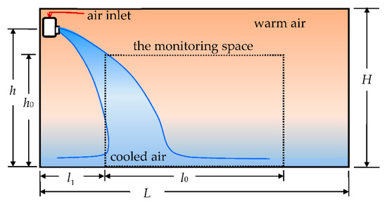
Figure 1.
Configuration of the room air-conditioning system at the early stages of operation and the flow formed by an inclined buoyant jet from the cold air leaving the device exit. The blue colour corresponds to cold air and orange to warm air. The dotted line shows the space where the air temperature has been monitored.
The above description of the phenomenon shows that the cold airflow originating from the air-conditioning device forms an inclined buoyant jet in an initially density and temperature uniform ambient, which progressively becomes stratified tending to obtain again uniform conditions with temperature equal to that of the exit air from the device. Therefore, this is a well-known filling box operation in conjunction with the inclined positively buoyant jet. For simplicity reasons, an inclined plane buoyant jet is considered, which has been mathematically described and tested [45,47,48]. This model constitutes the 2D mode of the EMA integral model, which in the context of the present study is supplemented with the additional ability to treat flow and mixing in stratified environments.
2.1. Mathematical Description
2.1.1. General Description, Assumptions, and Approximations
The 2D source of cooled air is considered to have a slot with D, air exit velocity w0 and temperature T0. The initial room air temperature before the air-conditioning operation is Ta0 > T0. The corresponding air densities are ρ0 and ρa0, where ρ0 > ρa0. The momentum due to exit velocity drives the cooled air in the direction of the outlet inclination with respect to the horizontal plane, while the buoyant forces due to density differences move the heavier cooled air downward. The combined result of these motions is a curvilinear air motion, the well-known flow of inclined plane turbulent buoyant jet in a stratified environment shown in Figure 2. The buoyant jet starts with the kinematic fluxes of volume μ0 = D w0, momentum m0 = D w02, and buoyancy β0 = g0′μ0, where g0′ = g(ρ0 − ρa0)/ρ0 is the effective acceleration of gravity. Along with the buoyant jet travel, the volume flux is increased due to entrained flow from the environment, momentum flux changes due to the combined competition among inertial, buoyancy, and turbulent viscosity forces, while the buoyancy flux may usually decrease or conserved, depending on the environmental conditions (uniform or density stratified). If the air conveyed by the buoyant jet reaches the bottom boundary or it is intermediately trapped due to stratification, it moves slowly horizontally on the denser layer without any mixing. The latter effect is termed the entrainment blocking effect [49]. For enabling velocity, density, and temperature monitoring at any point of the 2D flow field, two orthogonal coordinate systems are defined; a main Cartesian system O(y, z) and a local curvilinear one Ol(ψ, ξ), as shown in Figure 2. In this figure, the flow and mixing field configuration is also shown. Basics of orthogonal curvilinear coordinate systems are provided by Batchelor [50]. The case of buoyant jet trapping presented in Figure 2 occurs when the jet density ρ becomes equal to the ambient density ρa. At this level (equilibrium level in Figure 2), the local effective acceleration of gravity g′ = g(ρ − ρa)/ρ0 becomes zero, but the buoyant jet continues moving due to its inertia up to the maximum height , where opposite buoyant force occurs (ρ < ρa) and its motion is reversed. Thus, the buoyant jet oscillates around with Brunt–Väisälä frequency, while it is spreading horizontally sideways at this level [46].
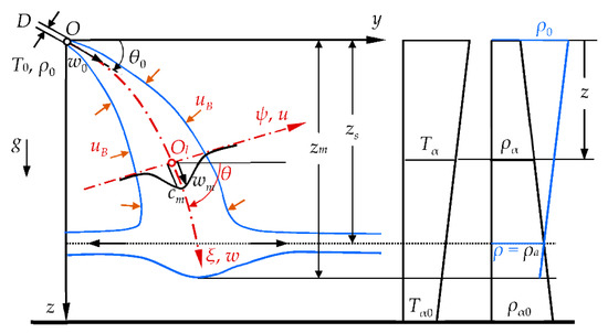
Figure 2.
Configuration of the flow and mixing field of an inclined buoyant jet in a stratified environment.
The most significant parameters that describe the behaviour of an inclined buoyant jet into a linearly stratified ambient are:
- The densimetric Froude number, defined as . In general, high values of Froude number indicate that the flow is governed by inertial forces (jet-like behaviour), while low enough values indicate that buoyant forces dominate the flow (plume-like behaviour).
- The stratification parameter, defined as . This is directly related to the Brunt–Väisälä frequency , giving the frequency of oscillations of the trapped buoyant jet at the equilibrium level [46]. The parameter shows the stratification strength, where is the thermocline layer height. Stratification is strong if , moderate if and weak if [49].
- The characteristic length scale defined by [51]. It is herein used to normalise the geometric distances. The independent variables ψ, ξ and z are normalised to the dynamic distances , and . For either plane or round buoyant jets, experimental evidence has shown that a jet-like behaviour of flow occurs when , while a plume-like behaviour is obtained when .
- For the dependent variables of velocity, relative concentration and relative temperature, the scale is used, where stands for the corresponding value of variable at the exit.
The derivation of the conservation equations governing the flow and mixing of inclined buoyant jets is based on the usual assumptions and approximations described by Yannopoulos & Noutsopoulos [52,53] and Bloutsos & Yannopoulos [54] along with the addition of the second-order terms of the turbulence contribution to momentum and buoyancy fluxes [51,55]. More details are given by Yannopoulos & Bloutsos [45] and Bloutsos & Yannopoulos [47] concerning such flows within uniform environments. The derivation regarding stratified environments obeys the same rules with the difference in the definition of the above local parameter g′ and its value at the exit, . This new definition is more general and affects the definitions of the dimensionless relative concentration and relative temperature. Thus, the relative concentration definition is . Assuming that the density differences are small enough for the Boussinesq approximation to be valid and applying the ideal gas law for constant pressure, the following equalities are obtained: , where temperatures are in K. Thus, , and , correspondingly. In this manner, for practical purposes, the tracer concentration based on densities is about equal to the concentration based on temperatures, . The temperature may be any value of the space of calculation. For the present study, the most appropriate value is the mean temperature corresponding to the buoyant jet transverse cross-section. Thus, is computed using the bulk concentration, which is defined as the inverse of the bulk dilution, i.e., , where . This is necessary for feeding air of mean temperature in the spreading layer. It is noticed that and vary in the range from 0 up to 1. The temperatures for the case studied must satisfy the expression . For simplicity reasons, the inclined buoyant jet is assumed to be symmetrical with respect to the curvilinear axis .
2.1.2. Governing Equations of Flow and Temperature Field
The partial differential equations (PDE) of continuity, momentum in ψ and ξ direction, as well as the tracer conservation, regarding a 2D inclined turbulent buoyant jet flowing on the plane yz, are:
where u and w are the mean velocity components in the directions ψ and ξ of the curvilinear coordinate system; is the scale factor of the coordinate system; is the local inclination of the axis; is the relative concentration as defined previously; the , , are the mean values of the local fluxes due to turbulence fluctuations of , and ; is the mean turbulent shear stress; is the dynamic pressure; the last term on the right of Equation (4) is the new term mentioned previously, which is incorporated in EMA and describes the state of the fluid environment, being initially uniform and becoming gradually stratified. It is noted that the system of Equations (1)–(4) describes the phenomenon at steady-state, but in the present study the solution of the unsteady phenomenon is performed as a problem of quasi-steady state. It must be also noted that the coordinate systems are clockwise, but equations are written for normal counterclockwise systems to avoid confusion. Therefore, the reader should treat independent variables of equations and definitions, z, ψ, ξ, θ, as being negative.
2.1.3. Integration of PDE on the Buoyant Jet Cross-Section
The integration of Equations (1)–(4) is based on the definition of the boundary conditions and the transverse profile functions for velocities and concentration. The following boundary conditions should be satisfied by the Equations (1)–(4):
where is the physical half width of the plane buoyant jet, which is about equal to ; is the spreading nominal width of the inclined plane buoyant jet, defined as the transverse distance from the jet centreline where ; is the spreading rate coefficient, which is constant and equal to 0.132; is the entrainment velocity given by Yannopoulos [51]:
where .
To enable integration and concise formulation of the ordinary differential equations (ODE), the following local kinematic fluxes of volume, momentum, weight deficit and buoyancy are used: ; ; ; and , correspondingly. Factors and introduce the turbulence contributions to the momentum and buoyancy fluxes; factors ,, , are the corresponding shape factors used to correct the calculation of the fluxes at the core region, where the Gaussian profiles are not valid. More details are given by Yannopoulos and Bloutsos [45]. These fluxes are the integrals from to of the transverse variations (Gaussian profiles) of the variables included in the relevant local fluxes. These profiles are and for the transverse variation of axial velocities and concentrations, correspondingly. They are used to integrate the PDE (1)–(4) along with the boundary conditions (5) and entrainment expression (6).
The final forms of ODE obtained after integration of the above PDE are:
2.1.4. Application to a Room Air-Conditioning
The experimental room, where temperature measurements have been made by He et al. [56], is used for the present model application. A sketch of the room is shown in Figure 1. The room has a length L = 5.20 m, width B = 3.50 m, and height H = 2.67 m. An air-conditioning device is fixed at the smaller sidewall of the room and at the height of m. The distance of the device outlet from this wall is not given; it is taken equal to 0.25 m. Thus, the available room length is m. At the central area of the room, the measurement sensors had been located covering an area of 3.00 m long, 1.50 m wide, with height m. The distance of this area from the smaller sidewalls is m and 1.00 m from the longer ones. The volume of the room is 48.6 m3. The room is an inner chamber, thermally well insulated, located within a laboratory. Initially, before the air conditioning device operation, the air temperature of the room was uniform at 35 °C.
The air-conditioning device provides an airflow rate of 0.215 m3/s with exit velocity 3 m/s and temperature 27 °C, which recirculated the room air, sinking it from the ceiling region at 35 °C and injecting it cooler to the room at the level m above floor. The retention time or the time to pass all the air volume from the air-conditioning device is s. The researchers He et al. [56] have found a time of about 31 min for temperature stabilisation and they calculated a cooling rate of 0.269 °C/min.
In Appendix A, the 2D mode of the integral model EMA equipped with Equation (10) is qualified by comparing its predictions for vertical and inclined plane buoyant jets in linearly stratified environments with experimental measurements available in the literature. Therefore, it can be successfully applied to predict plane buoyant jets of positive or negative buoyancy [47]. In general, the results agree well with available experimental data. In the context of the present study, this mode of EMA is implemented to predict the air temperature transition during air-conditioning of the room environment. Thus, the considered exit area of the device has a length equal to the sidewall (3.50 m); the slot exit is D = 0.0204 m to keep the same area, exit velocity and thermal load. Consequently, the flowrate per length is m2/s. The strength of stratification is moderate, as . Five inclination angles of the exit velocity, shown in Figure 2, are examined: 15, 30, 45, 60, and 75°.
The solution is schematically configured in Figure 3 and proceeds as follows:
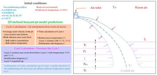
Figure 3.
Configuration sketch of the bottom-up approach used to solve the quasi-steady phenomenon of a room air conditioning. The colours show the cooling transition from warm air (red) to cool air (blue).
- Step 1. For a uniform room-air temperature of °C, the model runs for the above-prescribed exit and room conditions and predicts the trajectory of the buoyant jet. When the buoyant jet meets the room floor, is deflected and spreads horizontally sideways for 2 s up to fill a layer of height m. The layer temperature is , because the buoyant jet during its passage entrains warmer air from the room and mixes it with the produced cool air. Since , for the layer density is and, thus, this layer remains at the bottom as heavier than the above room air; note that the buoyant jet behaviour is plume-like near the bottom with insignificant momentum [9]. The room air stratification is now started with a Brunt–Väisälä frequency . At this step, the mean air temperature of the buoyant jet at the level of this layer is increased to due to entrainment. The total time needed from the air-conditioning start up to this point is considered as one cycle of operation.
- Step 2. The model runs from the beginning, but, as it approaches the bottom wall, it entrains and mixes air with temperature . Thus, its temperature and its density become and , correspondingly, while the buoyant jet temperature becomes . For the reasons described in Step 1, it pushes up the previous layer and takes its position, forming another stratified region with frequency . This is the second cycle of the procedure.
- Step 3. The procedure continues as described in Step 2 up to fill with layers the room space from the floor up to the exit level of the air-conditioning device. The total time needed for integrating the whole procedure is calculated as described in Step 1, accounting for all cycle steps. The air stratification reduces the buoyant jet momentum, and the flow is governed more and more by buoyant forces. This reason causes the buoyant jet to approach the bottom wall at the last step earlier than at the first step. However, no jet trapping happened during the runs for the inclination angles examined. It is observed that, at the last step, the room air temperature becomes uniform and equal to the exit temperature.
The limitations of the proposed procedure arise from the use of the model two-dimensionality in a confined room space. Consequently, the model can predict the variations of the mean axial velocity and mean temperature along the central area of the room longitudinal cross-section yz, while it cannot predict the variations near sidewall and ceiling boundaries. Another limitation is the available room length , which should be greater than of the jet outer boundary when it meets the room floor (), where ymax = y + Bwsinθ depends on the exit parameters of velocity , inclination angle , Froude number and distance ξ or alternatively y. Thus, for given values of , and .
3. Results and Discussion
3.1. Buoyant Jet Characteric Variations
Figure 4 shows the variation of the buoyant jet trajectories from the exit level () of the air-conditioning device up to approaching the layer of the first cycle (). As the stratification of the room air progresses upwards, it is observed increased bending over of the buoyant jet, which approaches the bottom earlier than at the beginning. This event is more and more pronounced as the initial jet inclination reduces. The total time needed to integrate the uniform room-air temperature to be equal to the exit temperature of 27 °C depends on the inclination angle and it is given in Table 1 along with the lengths and of the trajectories, cycle times and at the first and last simulation cycle, and total time for all cycles of simulation, correspondingly. The cycle time calculation is based on the average axial velocity at the jet cross-section of the buoyant jet, as it is in consent to the bulk dilution.
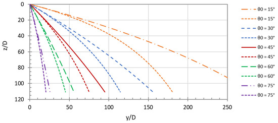
Figure 4.
Dimensionless buoyant jet trajectories at the first cycle of air conditioning operation and at the last cycle for the inclination angles examined. The results for the last cycle are shown with the same colour as for the first cycle colour, but with lines of the smallest dash.

Table 1.
For each initial inclination angle examined, trajectory lengths and of the buoyant jet at the first and the last simulation cycle, along with the corresponding total times and , as well as the total duration of all cycles, for temperature stabilisation of the room air at 27 °C.
From the data given in Table 1, it is indicated that the higher the inclination of the exit, the smaller the trajectory length and time needed the buoyant jet to meet the bottom wall. The total time needed to stabilise the air temperature follows the same behaviour. This time varies from s for to more than s for . As previously given, He at al. [56] reported a stabilisation time about 31 min, i.e., 1860 s, which is little greater than the total time computed from the present study. This may be attributed to the use of an inclination angle around 15° in conjunction with the fact that the above researchers had considered that temperature stabilisation occurred in the whole air volume of the room.
Figure 5a shows the variation of the normalised dimensionless centreline velocity of the buoyant jet with respect to the normalised trajectory length . It is observed that, irrespective from the exit angle and cycle of simulation, the velocities show approximately equal values up to about 30% of initial passage following the same decay slope, which is −0.5 in a log-log presentation. This slope is significantly reduced as the buoyant jet approaches the bottom wall. The slope −0.5 corresponds to a jet-like behaviour [51]. The decay slopes and of the corresponding centreline velocities and concentrations, calculated at the last cycle for the initial inclination angles examined are provided in Table 2.
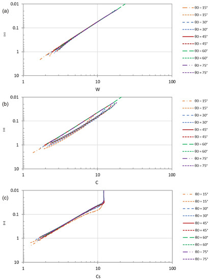
Figure 5.
Variation of the normalised (a) dimensionless centreline buoyant jet velocity ; (b) centreline concentration ; and (c) bulk concentration with respect to the normalised trajectory length for the first and last cycle of air conditioning operation, for the inclination angles examined. The results for the last cycle are shown with same colour as for the first cycle’s, but with lines of the smallest dash.
Table 2.
Decay slopes of centreline velocity and concentration calculated at the last cycle of simulation for initial inclination angles examined.
It is shown that the decay slopes are increased with decreasing the inclination angles. The value −0.134 approaches the zero slope, which corresponds to the plume-like behaviour of plane buoyant jets [51].
Figure 5b shows the variation of the normalised centreline concentration with respect to the normalised trajectory length for the first and last cycle of simulation. It is observed that, irrespective of the exit angle and cycle of simulation, the centreline concentrations are approximately equal at the same distances, and they decay with the same slope, which equals to −0.51, regarding the first cycle of simulation. This slope is approximately equal to the slope of the jet-like behaviour of plane buoyant jets [51]. Unlike for velocities, the concentrations depart from the initial decay to lower values due to stratification, then they follow a similar decay rate to the initial one for a while and finally tend to a decay slope approximately equal to −1, as shown in Table 2. The slope −1 of concentrations in a log-log diagram presentation corresponds to the plume-like behaviour of plane buoyant jets [51].
Figure 5c shows the variation of the normalised bulk concentration , which is the inverse of the normalised bulk dilution. Unlike the decay slopes of centreline concentration, the decay slopes of bulk concentration show approximately the same behaviour along Ξ distance, irrespective of the simulation cycle, except , which shows some differences, since the buoyant jet meets the opposite sidewall before the floor.
3.2. The Transient State of the Room Air Temperatures
Figure 6 shows the variation of the mean air temperature of the buoyant jet cross-section with respect to the vertical distance from the exit of the air-conditioning device. It also shows the corresponding variation of the average room air temperature at the same level as the level of . is affected by the flowrate of the cooler air provided by the air-conditioning device, while is influenced by through the entrained room air by the buoyant jet.
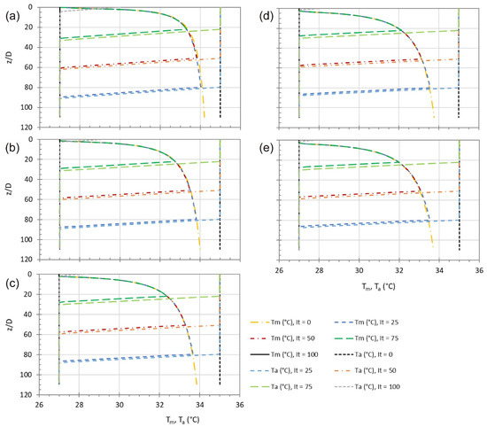
Figure 6.
Variation of the air temperatures and (°C) with respect to the dimensionless vertical distance from the exit of the air-conditioning device for the first cycle (it = 0) with uniform room air temperatures at 35 °C, the cycle after 25 cycle calculations (it = 25) and the cycles after 50, 75 and 100 cycle calculations for: (a) ; (b) ; (c) ; (d) ; and (e) . is the mean air temperature at the buoyant jet cross-section; and is the mean room air temperature outside the jet at the same level with . starts from °C and from °C. and are shown with the same colours and line modes for the same cycle, but the colour for is a little lighter than that for .
The entrained air is warmer than the jet air and their mixture obtains an intermediate temperature value. As explained in the previous section, the values of are computed through the bulk dilution and, thus , where is the centreline temperature value at the same distance ξ. The variation of these temperatures is provided in Figure 6 for five cycles of simulation (it = 0, 25, 50, 75, and 100) and each diagram (a), (b), (c), (d), and (e) corresponds to the initial inclination of the exit velocity of the air-conditioning device.
The temperature is initially (at the exit) equal to °C and then is increased with z, approaching °C for the first cycle (it = 0), where the room has a uniform temperature. It is observed from Figure 6 that the smaller the inclination angle, the closer the value of to . The temperature does not show any effect at the first cycle.
During the intermediate cycles, variation follows the same curve with that of the first cycle up to a distance z, where meets the sequence of the stratified layers that they have obtained the temperature of the air-conditioning and lowers rapidly to °C following the same cooling rate (thermocline) of thermocline. As expected, it is observed from Figure 6 that this event delays more in the initial cycle simulations, while it occurs in a shorter time at the last cycles, because the distance of the upper layer of the stratified sequence from the air-conditioning exit is gradually reduced.
Figure 7 shows the variation of the average values of the air temperatures and (°C) with respect to the cycles time. Averaging is applied to the region from the room floor up to the level of 1.90 m above the floor (Figure 1). This region is selected to compare the present result with the measurements carried out by He et al. [56] in the same region. As it is observed in Figure 7, regarding , the temperatures at the first simulation cycle show a variation depending on the exit velocity inclination . They are in the range from 33.92 to 33.12 °C, with the small value to correspond to and the high one to . Unlike , temperature has not changed yet. After about s and up to s, the temperatures and decay approximately linearly. It is observed that the higher the value of , the shorter the time for the room air to obtain the temperature of 27 °C provided by the air-conditioning device. The cooling rates and of and , correspondingly, show a dependence on and on cycles time.
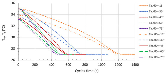
Figure 7.
Variation of the average values of air temperatures and (°C) with respect to the simulation cycles time, in the region from the room floor up to the level of 1.90 m above floor.
The values of the corresponding cooling rates (°C/min) in time intervals are provided in Table 3 with respect to . It is observed that the cooling rates are absolutely lower than of . The absolutely lowest value of is °C/min, which happens when , while it is increased up to the value of °C/min when . Regarding , the absolutely lowest value is °C/min when and it is increased up to the value °C/min when .
Table 3.
Cooling rates of the temperatures and during time intervals of the cycles for each inclination angle examined.
Based on the simulation performed by He et al. [56], the cooling rate was −0.269 °C/min, which is approximately equal to the corresponding absolutely lowest cooling rate of the predictions in the context of the present study (−0.266 °C/min). As explained previously, such a cooling rate should occur when the inclination angle of the exit velocity is about equal to 15°. It must be noticed that the times shown in Figure 7, concerning the stabilisation of the room air temperature, are shorter than times given in Table 1, because the results presented in Figure 7 represent the part of the room from the floor up to the level of 1.90 m, where measurements have been performed [56]. It is evident that this part gets the uniform temperature of 27 °C earlier than the whole space up to the height of 2.30 m of the exit of the air-conditioning device.
3.3. Brunt–Väisälä Frequency Presentation
It is interesting to note that the thermoclines are approximately equal to −0.02 °C/m, while it is not observed any stratification during the first cycle of simulation. We noticed that the thermocline of −0.02 °C/m equals the tropospheric sub-adiabatic ambient lapse rate (temperature inversion) of type E, which characterises moderate atmospheric stability [57]. Note that the minus sign is due to the use of a clockwise coordinate system. Since the height of layers is common to all the cases examined, it is expected that the thermoclines will start and finish at the same z levels, irrespective of the angle of inclination and the cycle of simulation, which agrees with the results shown in Figure 6 and Figure 8.
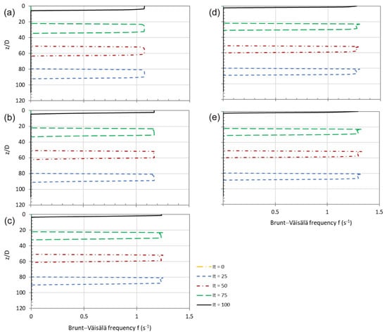
Figure 8.
Occurrences of Brunt–Väisälä frequency f (s−1) of the stratified layer sequence under the uniform room air temperatures with respect to the dimensionless vertical distance from the exit of the air-conditioning device for the cycles after 25 (it = 25), 50 (it = 50), 75 (it = 75) and 100 (it = 100) cycle calculations for: (a) ; (b) ; (c) ; (d) ; and (e) . Note that there is not any occurrence during the first cycle (it = 0).
Figure 8 presents four selected occurrences of the Brunt–Väisälä frequency f and its progress during the cycles of simulation. Since f is directly related to the stratification parameter or the thermocline occurrences, f is expected to behave in the same manner. All frequency occurrences agree completely with the occurrences and location to the thermoclines for the same cycle of simulation, irrespective of the initial inclination angle. It is observed in Figure 8 that the f values increase with the increase of the inclination angle of the exit velocity, while they remain constant during the time of the simulation cycles for the same inclination angle. The latter values are provided in Table 4.
Table 4.
Values of the Brunt–Väisälä frequency f during the simulation cycles for each inclination angle examined.
The frequency values included in Table 4 show that, in case of buoyant jet trapping, the jet maximum height will oscillate around the equilibrium level of zero buoyancy with frequencies from 1.07 to 1.32 s−1 for to 75°, correspondingly. However, as mentioned previously, no jet trapping occurred during simulation.
4. Conclusions
From the application of the integral model to simulate the transient phenomenon that occurs when a closed room, well insulated, with an air temperature of 35 °C, is air-conditioned with 27 °C air circulation of a flow rate of 0.215 m3/s, the most important points are identified, and the following conclusions are drawn:
- As shown by the results and the associated discussion, the integral model EMA equipped with the conservation of tracer (relative concentration or relative temperature) and satisfactorily qualified was finally appropriate to perform the present study. The technique proposed to treat the transient phenomenon as a quasi-steady-state along with EMA and the novel bottom-up approach to produce layers by the buoyant jet formed by the cool air leaving the air-conditioning device proved successful.
- It was certified by the model implementation that the most appropriate concentration to get reasonable results of the room air temperatures is based on the bulk dilution because it feeds the layers with the average air temperature of the near bottom cross-section of the buoyant jet.
- The simulation showed that a momentum-dominated buoyant jet within a uniform environment rather keeps this behaviour, while it gradually becomes buoyancy dominated within a stratified environment. Thus, although at the first cycle of simulation, when the room air is uniform, the buoyant jet has a nearly straight trajectory, at the last cycle of simulation, the trajectory bends over downward.
- The simulation time needed for stabilisation of the room temperature at 27 °C provided by the air-conditioning device is more than 28 min for 15° inclination angle of the jet exit; this result approximated closely the experimental time of 31 min.
- The cooling rates based on the average temperature of the buoyant jet cross-section, are 10 to 30% lower than the corresponding ones based on the room temperatures.
- The Brunt–Väisälä frequency occurring during the temperature transitions remains constant for the same inclination angle of the exit velocity. Its value is increased with increasing the inclination angle, ranging between 1.07 to 1.32 s−1.
- The model could be used for the evaluation of air-conditioning systems operating in closed rooms by recirculating the room air. Future studies could focus on simulating the heating of a room using air-conditioning systems or fan coils.
Author Contributions
Conceptualization, P.C.Y. and A.A.B.; methodology, P.C.Y.; software, P.C.Y.; validation, P.C.Y. and A.A.B.; formal analysis, P.C.Y. and A.A.B.; investigation, P.C.Y. and A.A.B.; writing—original draft preparation, P.C.Y.; writing—review and editing, P.C.Y. and A.A.B.; visualization, P.C.Y. and A.A.B. All authors have read and agreed to the published version of the manuscript.
Funding
This research received no external funding.
Institutional Review Board Statement
Not applicable.
Informed Consent Statement
Not applicable.
Data Availability Statement
The data generated and/or analysed during this study are available from the corresponding author on reasonable request.
Conflicts of Interest
The authors declare no conflict of interest.
Appendix A. Qualification of the 2D Mode of EMA
The 2D mode of the integral model EMA is herein used to predict several cases of both vertical and 45° inclined plane buoyant jets in linearly stratified environments. The level of the spreading layer and the dilution at this level are predicted. The results regarding the vertical buoyant jet cases are compared with the corresponding measurements provided by Wallace & Write [58] and shown in Figure A1a concerning the normalised spreading layer level and in Figure A1b concerning the normalized dilution .

Figure A1.
Vertical plane buoyant jet cases in linearly stratified environments: (a) Comparison of predicted to measured values of the normalised level of the spreading layer; and (b) comparison of predicted to measured values of the normalised dilution .
Concerning the 45° inclined buoyant jet cases, the results of the normalised level of the spreading layer and normalized dilution are compared with the corresponding measurements provided by Lee & Cheung [59] and shown in Figure A2a,b, correspondingly.
Figure A1a shows that predictions agree perfectly well to the experimental measurements. The agreement is also satisfactory regarding shown in Figure A1b except one case that may be ambiguous. This uncertain case represents the dilution of a vertical plane plume at the highest level measured by Wallace & Write [58]. Concerning the predictions of 45° inclined plane buoyant jet shown in Figure A2a, the comparison with the corresponding measurements provided by Lee and Cheung [59] is excellent for , while the predictions overestimate the measurements up to 10% (accuracy of 2nd order), except one case that prediction overestimation is 22% (accuracy of 1st order). In contrary, the agreement is very good regarding shown in Figure A2b, since the accuracy of all predictions is of 2nd order.

Figure A2.
Inclined plane buoyant jet cases in linearly stratified environments: (a) Comparison of predicted to measured values of the normalised level of the spreading layer; and (b) comparison of predicted to measured values of the normalised dilution .
Consequently, EMA can be satisfactorily to simulate either vertical or inclined plane buoyant jets in stratified environments.
References
- Baines, W.; Turner, J. Turbulent buoyant convection from a source in a confined region. J. Fluid Mech. 1969, 37, 51–80. [Google Scholar] [CrossRef]
- Turner, J.S. Buoyancy Effects in Fluids; Cambridge University Press: Cambridge, UK, 1973. [Google Scholar]
- Germeles, A. Forced plumes and mixing of liquids in tanks. J. Fluid Mech. 1975, 71, 601–623. [Google Scholar] [CrossRef]
- Worster, M.G.; Huppert, H.E. Time-dependent density profiles in a filling box. J. Fluid Mech. 1983, 132, 457–466. [Google Scholar] [CrossRef]
- Barnett, S.J. The Dynamics of Buoyant Releases in Confined Spaces. Ph.D. Thesis, University of Cambridge, Cambridge, UK, October 1991. [Google Scholar]
- Thomas, L.P.; Marino, B.M.; Tovar, R.; Castillo, J.A. Flow generated by a thermal plume in a cooled-ceiling system. Energy Build. 2011, 43, 2727–2736. [Google Scholar] [CrossRef]
- Cheng, Y.; Lin, Z. Experimental investigation into the interaction between the human body and room airflow and its effect on thermal comfort under stratum ventilation. Indoor Air 2016, 26, 274–285. [Google Scholar] [CrossRef]
- Yang, R.; Ng, C.S.; Chong, K.L.; Verzicco, R.; Lohse, D. Do increased flow rates in displacement ventilation always lead to better results? J. Fluid Mech. 2022, 932, A3. [Google Scholar] [CrossRef]
- Hunt, G.R.; Cooper, P.; Linden, P.F. Thermal stratification produced by jets and plumes in enclosed spaces. Build. Environ. 2001, 36, 871–882. [Google Scholar] [CrossRef]
- Kaye, N.B.; Hunt, G.R. Overturning in a filling box. J. Fluid Mech. 2007, 576, 297–323. [Google Scholar] [CrossRef]
- Kaye, N.B.; Hunt, G.R. Smoke filling time for a room due to a small fire: The effect of ceiling height to floor width aspect ratio. Fire Saf. J. 2007, 42, 329–339. [Google Scholar] [CrossRef]
- Van Sommeren, D.D.J.A.; Caulfield, C.P.; Woods, A.W. Turbulent buoyant convection from a maintained source of buoyancy in a narrow vertical tank. J. Fluid Mech. 2012, 701, 278–303. [Google Scholar] [CrossRef]
- Akhter, R.; Kaye, N.B. Experimental investigation of a line plume in a filling box. Environ. Fluid Mech. 2020, 20, 1579–1601. [Google Scholar] [CrossRef]
- Gladstone, C.; Woods, A.W. Detrainment from a turbulent plume produced by a vertical line source of buoyancy in a confined, ventilated space. J. Fluid Mech. 2014, 742, 35–49. [Google Scholar] [CrossRef]
- Bonnebaigt, R.; Caulfield, C.P.; Linden, P.F. Detrainment of plumes from vertically distributed sources. Environ. Fluid Mech. 2016, 18, 3–25. [Google Scholar] [CrossRef]
- Kaye, N.B.; Cooper, P. Source and boundary condition effects on unconfined and confined vertically distributed turbulent plumes. J. Fluid Mech. 2018, 850, 1032–1065. [Google Scholar] [CrossRef]
- Cooper, P.; Hunt, G.R. The ventilated filling box containing a vertically distributed source of buoyancy. J. Fluid Mech. 2010, 646, 39–58. [Google Scholar] [CrossRef][Green Version]
- Wong, A.B.D.; Griffiths, R.W. Stratification and convection produced by multiple turbulent plumes. Dyn. Atmos. Ocean. 1999, 30, 101–123. [Google Scholar] [CrossRef]
- Yin, S.; Li, Y.; Fan, Y.; Sandberg, M. Unsteady large-scale flow patterns and dynamic vortex movement in near-field triple buoyant plumes. Build Environ. 2018, 142, 288–300. [Google Scholar] [CrossRef]
- Yin, S.; Li, Y.; Fan, Y.; Sandberg, M. Experimental investigation of near-field stream-wise flow development and spatial structure in triple buoyant plumes. Build Environ. 2019, 149, 79–89. [Google Scholar] [CrossRef]
- Yin, S.; Fan, Y.; Sandberg, M.; Li, Y. PIV based POD analysis of coherent structures in flow patterns generated by triple interacting buoyant plumes. Build Environ. 2019, 158, 165–181. [Google Scholar] [CrossRef]
- Cariteau, B.; Brinster, J.; Tkatschenko, I. Experiments on the distribution of concentration due to buoyant gas low flow rate release in an enclosure. Int. J. Hydrog. Energy 2011, 36, 2505–2512. [Google Scholar] [CrossRef]
- Cariteau, B.; Tkatschenko, I. Experimental study of the effects of vent geometry on the dispersion of a buoyant gas in a small enclosure. Int. J. Hydrog. Energy 2013, 38, 8030–8038. [Google Scholar] [CrossRef]
- Gupta, S.; Brinster, J.; Studer, E.; Tkatschenko, I. Hydrogen related risks within a private garage concentration measurements in a realistic full scale experimental facility. Int. J. Hydrog. Energy 2009, 34, 5902–5911. [Google Scholar] [CrossRef]
- Cariteau, B.; Tkatschenko, I. Experimental study of the concentration build-up regimes in an enclosure without ventilation. Int. J. Hydrog. Energy 2012, 37, 17400–17408. [Google Scholar] [CrossRef]
- De Stefano, M.; Rocourt, X.; Sochet, I.; Daudey, N. Hydrogen dispersion in a closed environment. Int. J. Hydrog. Energy 2018, 44, 9031–90400. [Google Scholar] [CrossRef]
- Chen, M.; Zhao, M.; Huang, T.; Ji, S.; Chen, L.; Chang, H.; Li, X. Measurements of helium distributions in a scaled-down parking garage model for unintended releases from a fuel cell vehicle. Int. J. Hydrog. Energy 2020, 45, 22166–22175. [Google Scholar] [CrossRef]
- Cardoso, S.S.S.; Woods, A.W. Mixing by a plume in a confined stratified region. J. Fluid Mech. 1993, 250, 277–305. [Google Scholar] [CrossRef]
- Bloomfield, L.J.; Kerr, R.C. Turbulent fountains in a confined stratified environment. J. Fluid Mech. 1999, 389, 27–54. [Google Scholar] [CrossRef]
- Mott, R.W.; Woods, A.W. On the mixing of a confined stratified fluid by a turbulent buoyant plume. J. Fluid Mech. 2009, 623, 149–165. [Google Scholar] [CrossRef][Green Version]
- Cleaver, R.P.; Marshal, M.R.; Linden, P.F. The build-up of concentration within a single enclosed volume following a release of natural gas. J. Hazard. Mater. 1994, 36, 209–226. [Google Scholar] [CrossRef]
- Kaye, N.B.; Ji, Y.; Cook, M.J. Numerical simulation of transient flow development in a naturally ventilated room. Build. Environ. 2009, 44, 889–897. [Google Scholar] [CrossRef]
- Yang, X.; Zhong, K.; Kang, Y.; Tao, T. Numerical investigation on the airflow characteristics & thermal comfort in buoyancy-driven natural ventilation rooms. Energy Build. 2015, 109, 255–266. [Google Scholar] [CrossRef]
- El-Amin, M.F.; Sun, S.; Heidemann, W.; Müller-Steinhagen, H. Analysis of a turbulent buoyant confined jet modeled using realizable k–ɛ model. Heat Mass Transf. 2010, 46, 943–960. [Google Scholar] [CrossRef]
- George, A.M.; Kay, A. Numerical simulations of a line plume impinging on a ceiling in cold fresh water. Int. J. Heat Mass Transf. 2017, 108, 1364–1373. [Google Scholar] [CrossRef]
- Hattori, T.; Armfield, S.W.; Kirkpatrick, M.P. Transitional ventilated filling box flow with a line heat source. Int. J. Heat Mass Transf. 2012, 55, 3650–3665. [Google Scholar] [CrossRef]
- Gao, X.; Li, A.; Yang, C. Study on thermal stratification of an enclosure containing two interacting turbulent buoyant plumes of equal strength. Build Environ. 2018, 141, 236–246. [Google Scholar] [CrossRef]
- Cao, G.; Kurnitski, J.; Ruponen, M.; Seppänen, O. Experimental investigation and modelling of a buoyant attached plane jet in a room. Appl. Therm. Eng. 2009, 29, 2790–2798. [Google Scholar] [CrossRef][Green Version]
- Cao, G.; Sivukari, M.; Kurnitski, J.; Ruponen, M. PIV measurement of the attached plane jet velocity field at a high turbulence intensity level in a room. Int. J. Heat Fluid Flow. 2010, 31, 897–908. [Google Scholar] [CrossRef]
- Ji, K.; Cai, W.; Zhang, X.; Wu, B.; Ou, X. Modeling and validation of an active chilled beam terminal unit. J. Build. Eng. 2019, 22, 161–170. [Google Scholar] [CrossRef]
- Filipsson, P.; Trüschel, A.; Gräslund, J.; Dalenbäck, J.-O. Modelling of rooms with active chilled beams. J. Build. Perform. Simul. 2020, 13, 409–418. [Google Scholar] [CrossRef]
- Wu, B.; Cai, W.; Chen, H.; Ji, K. Experimental investigation on airflow pattern for active chilled beam system. Energy Build. 2018, 166, 438–449. [Google Scholar] [CrossRef]
- Cao, G.; Kurnitski, J.; Mustakallio, P.; Seppänen, O. Active Chilled Beam Wall Jet Prediction by the Free Convection Model. Int. J. Vent. 2008, 7, 169–178. [Google Scholar] [CrossRef]
- Nielsen, P.V.; Restivo, A.; Whitelaw, J.H. The Velocity Characteristics of Ventilated Rooms. J. Fluids Eng. 1978, 100, 291–298. [Google Scholar] [CrossRef]
- Yannopoulos, P.C.; Bloutsos, A.A. Escaping mass approach for inclined plane and round buoyant jets. J. Fluid Mech. 2012, 695, 81–111. [Google Scholar] [CrossRef]
- Lee, J.H.W.; Chu, V.H. Turbulent Jets and Plumes—A Lagrangian Approach; Kluwer Academic Publishers: Boston, MA, USA, 2003; ISBN 1-4020-7520-0. [Google Scholar]
- Bloutsos, A.A.; Yannopoulos, P.C. Curvilinear coordinate system for mathematical analysis of inclined buoyant jets using the integral method. Math. Probl. Eng. 2018, 2018, 3058425. [Google Scholar] [CrossRef]
- Bloutsos, A.A.; Yannopoulos, P.C. Revisiting Mean Flow and Mixing Properties of Negatively Round Buoyant Jets Using the Escaping Mass Approach (EMA). Fluids 2020, 5, 131. [Google Scholar] [CrossRef]
- Wallace, R.B.; Sheff, B.B. Two-dimensional buoyant jets in two-layer ambient fluid. J. Hydraul. Eng. 1987, 113, 992–1005. [Google Scholar] [CrossRef]
- Batchelor, G. An Introduction to Fluid Dynamics; Cambridge University Press: Cambridge, UK, 2000; ISBN 9780511800955. [Google Scholar]
- Yannopoulos, P.C. An improved integral model for plane and round turbulent buoyant jets. J. Fluid Mech. 2006, 547, 267–296. [Google Scholar] [CrossRef]
- Yannopoulos, P.C.; Noutsopoulos, G.C. Interaction of vertical round turbulent buoyant jets—Part I: Entrainment restriction approach. J. Hydraul. Res. 2006, 44, 218–232. [Google Scholar] [CrossRef]
- Yannopoulos, P.C.; Noutsopoulos, G.C. Interaction of vertical round turbulent buoyant jets—Part II: Superposition method. J. Hydraul. Res. 2006, 44, 233–248. [Google Scholar] [CrossRef]
- Bloutsos, A.A.; Yannopoulos, P.C. Round turbulent buoyant jets discharged vertically upwards forming a regular polygon. J. Hydraul. Res. 2009, 47, 263–274. [Google Scholar] [CrossRef]
- Yannopoulos, P.C. Advanced integral model for groups of interacting round turbulent buoyant jets. Env. Fluid Mech 2010, 10, 415–450. [Google Scholar] [CrossRef]
- He, L.; Zhao, S.; Xu, G.; Wu, X.; Xie, J.; Cai, S. Prediction and evaluation of dynamic variations of the thermal environment in an air-conditioned room using collaborative simulation method. Energies 2021, 14, 5378. [Google Scholar] [CrossRef]
- Pasquill, F.; Smith, F.B. Atmospheric Diffusion, 3rd ed.; Ellis Horwood: Cambridge, UK, 1983. [Google Scholar]
- Wallace, R.B.; Wright, S.J. Spreading layer of two-dimensional buoyant jet. J. Hydraul. Eng. 1984, 110, 813–828. [Google Scholar] [CrossRef]
- Lee, J.H.W.; Cheung, V.W.L. Inclined plane buoyant jet in stratified fluid. J. Hydraul. Eng. 1986, 112, 580–589. [Google Scholar] [CrossRef]
Publisher’s Note: MDPI stays neutral with regard to jurisdictional claims in published maps and institutional affiliations. |
© 2022 by the authors. Licensee MDPI, Basel, Switzerland. This article is an open access article distributed under the terms and conditions of the Creative Commons Attribution (CC BY) license (https://creativecommons.org/licenses/by/4.0/).