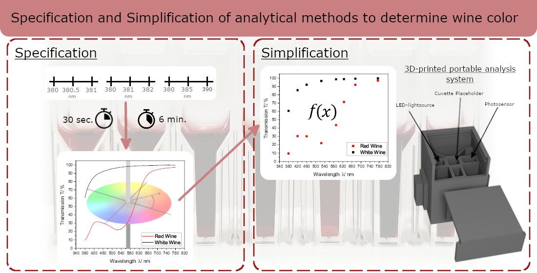
Specification and Simplification of Analytical Methods to Determine Wine Color

Abstract

The color of wine is an important quality parameter essential for the first impression of consumers. The International Organization of Vine and Wine (OIV) recommends two methods to describe wine color: color calculation according to Glories and the determination of coordinates in the CIE L*a*b* color space. The measurement of wine color is often not feasible for winemakers because the required instrumentation is expensive and bulky. In this study, the influence of photometer settings on the calculated color was investigated based on 14 wines. Furthermore, the CIE L*a*b* and Glories system were compared using 56 red and 56 white wines. Photometer settings were found to influence the reproducibility of color determination. In addition, CIE L*a*b* system do not correlate in all wines with the Glories system and Glories probably provides less information about wine color. Using interpolation, CIE L*a*b* coordinates were calculated from single wavelength measurements taken by a small-sized and inexpensive portable analysis system, which could be used by winemakers in the future.

1. Introduction

Color has a significant influence on the perceived quality of wine, altering the perception of aroma, taste and mouthfeel [1]. White wine dyed red was described using the olfactory attributes typical for red wine in contrast to the undyed white wine, which was perceived as having the olfactory attributes typical for white wine [2]. Given its influence on consumer perception, wineries aim to manage the wine color already during the production process to match consumer expectations with their final products. Objective methods and reliable devices are necessary to measure wine color during the winemaking process.

According to Grassmann’s laws, color can be described using three independent parameters [3]. These can be a primary color, the color intensity and the white intensity, or three primary valances, e.g., red, green, and blue [3]. There are two established methods to describe the color of wine.The first is the Glories method, which uses absorbance values at wavelengths of 420 nm, 520 nm and 620 nm, leading to a yellow, red and blue color impression for the observer [4,5]. However, variance of the human eye and the influence of surrounding light on color perception are not considered in the Glories calculations. Because of this, the Commission Internationale de L’Eclairage (CIE) defined the CIE standard system, which is a color space based on the color coordinates of X, Y and Z. The calculation of these coordinates is more complex, requiring a complete transmission spectrum in the visible range (380–780 nm). Furthermore, a standard observer [6] and a standard illuminant [7] are needed for calculation, which include the influence of the sensitivity of the human eye for different colors and the surrounding light on color perception. The standard observer is based on experimental work [8,9,10,11], where the spectral sensitivity of the eye for the three primary valances red, green and blue was investigated. The standard illuminant defines power distribution of standardized light sources, for example natural daylight on a sunny day [7]. The CIE XYZ system allows the objective and reproducible determinations of color, but colors in this system are not visually equidistant [12], meaning the Euclidean distance (ΔE) between two colors in this space does not correlate with the perceived color difference [13]. The CIE L*a*b* color space aims to achieve visual equidistance [12]. The International Organization of Vine and Wine (OIV) recommends the Glories and the CIE L*a*b* system for color determination in wine [14,15].

Regarding the CIE L*a*b* system, the OIV recommends to record transmission spectra in 5 nm steps, in the following mentioned as data intervals. However, it is unclear whether a data interval of 5 nm is optimal. While the CIE L*a*b* method, as described by the OIV, is popular in wine research, other versions of this method are used. Publications throughout the years have used data intervals of 1 nm, 2 nm or 10 nm for transmission measurements [16,17,18]. To evaluate this, an Analysis of Variance (ANOVA) and Bartletts test was used. No other requirements for technical parameters such as scan speed are given. It is not clear whether these photometer settings have an influence on the resolution, i.e., the ability to distinguish samples, and the reproducibility of the measurement.

Methods to assess wine color require expensive equipment as well as technical personnel to operate and maintain it in a laboratory environment. Therefore, a cheaper and easier, yet reliable, method to measure and calculate the color of wine is needed. In recent years, interest among wine producers in portable photometers has grown. Two basic modes of operation are available. The first mode of operation includes a broadband light source (e.g., white light LEDs, tungsten) and light dispersing elements such as prisms [19,20] and diffraction gratings [21], which are often combined with other optical elements, including lenses [20,22,23,24,25,26,27,28,29,30,31,32,33,34,35] or light guides [19]. This first mode of operation allows the capture of a complete transmission spectrum, though the optical elements required are expensive and must be aligned accurately. The second mode of operation uses a light source at a specific wavelength, such as a light emitting diode (LED) [36,37,38,39]. With this light source, an inexpensive light sensor, like a photodiode [37], -transistor [38] or -resistor [39] can be used. This second mode of operation is less costly, but such a photometer cannot be used to record a complete transmission spectrum, which is why it cannot be used for the CIE L*a*b* color calculation, as recommended by the OIV without further data processing. To calculate the CIE L*a*b*, coordinates from single wavelength measurements based on empirical methods are based on outdated standards, for example another standard observer or illuminant. Furthermore, these methods are not applicable in the same extent for every wine.

The overall objectives of this study are to specify technical parameters for reproducible wine color determination, to compare different methods for wine color determination, and to implement the CIE L*a*b* coordinate determination without expensive and bulky equipment. The first goal was to examine the influence of the photometer ‘data interval’, which must be set to record transmission spectra for the calculation of the CIE L*a*b* coordinates. Furthermore, the influence of the photometer setting ‘scan speed’ was investigated. The second goal was to determine whether the Glories and CIE L*a*b* systems are correlated, since both are commonly used and recommended. Older publications, which correlated the Glories method with the CIE L*a*b* color space, used the CIE 1931 2°-standard observer, the standard illuminant C or different pathways of cuvettes [17,40]. The current standard is the CIE 1964 10°-standard observer in combination with the standard illuminant D65, referred to a 10 mm pathway cuvette [12]. The third goal of this study was to develop a calculation method to determine CIE L*a*b* coordinates based on single wavelength transmission measurements instead of using a complete transmission spectrum. Approaches to derive CIE L*a*b* coordinates from these measurements were investigated either by direct correlation or by interpolation. For direct correlation, empirical methods after Ayala et al. [41] and Hardy et al. [42] were performed. Furthermore, different interpolation methods, namely Cubic splines and Lagrange and Sprague interpolation were investigated”. To reach the best approximation to the method according to the OIV, the calculated values were compared with data from the established laboratory method. The calculation methods were transferred to an inexpensive portable analysis system, which should allow portable on-site measurements.

2. Materials and Methods

2.1. Wines

The sample set consisted of 56 commercial red wines (Table S1) and 56 commercial white wines (Table S2). The red wines were produced from eight grape varieties, grown in eight countries during the vintages 2012 to 2021. The white wines were from six varieties, seven countries, and vintages from 2013 to 2021. Prices were between 5 and 20 €, a range considered average for wine on an international level [43,44]. The wines were selected to consider major wine producing countries [45], important grape varieties [46], and vintages that are currently available in the commercial wine trade, with the goal of representing the diversity of wine color.

2.2. Specification of Photometer Settings to Obtain CIE L*a*b* Coordinates

To specify technical parameters for wine color measurement, spectra from 300 to 900 nm of seven Merlot wines and seven Chardonnay wines were recorded with the data intervals of 0.5, 1, and 5 nm in combination with scan speeds of 100 and 1000 nm/min. Further technical parameters are given in Table S3. The red wines were measured in a 1 mm flow cuvette and the white wines in a 10 mm cuvette. To comply with the Lambert Beer law and with the recommendation of the CIE and OIV [7], the red wine spectra were corrected to a 10 mm pathway before CIE L*a*b* calculation. Triplicate measurements were conducted on a double beam photometer (V-730, JASCO, Tokyo, Japan). The CIE L*a*b* coordinates were extracted from the spectra between 380 and 780 nm in combination with the 10°-standard observer and D65 standard illuminant according to the CIE [7]. Experiments were repeated on another double beam photometer with a different monochromator and a different detector system (Varian Cary 100, Agilent, Santa Clara, CA, USA) but with comparable settings to investigate the influence of different photometers on the color calculation of wine.

The individual CIE L*a*b* coordinates of the seven wines of one grape variety were averaged, yielding the mean CIE L*a*b* coordinates for the grape variety (Equation (1)).

$$\overline{L^{*}}=\frac{\sum L_i^{*}}{n},\overline{a^{*}}=\frac{\sum a_i^{*}}{n},\overline{b^{*}}=\frac{\sum b_i^{*}}{n}$$

(1)

For each wine, ΔE was then calculated from its individual CIE L*a*b* coordinates and the mean CIE L*a*b* coordinates for the variety (Equation (2)).

$$\Delta E=\sqrt{{(\overline{L^{*}}-L_i^{*})}^2+{(\overline{a^{*}}-a_i^{*})}^2+{(\overline{b^{*}}-b_i^{*})}^2}$$

(2)

To assess the influence of data interval and scan speed on the resolution, which is here the ability to distinguish wines by color, and to assess the reproducibility of measurements, the sum of squared deviations (SSD) was calculated for every repetition separately (Equation (3)). Subsequently, the mean SSD (n = 3) was calculated reflecting the ability to distinguish wines by color and the standard deviation reflects the reproducibility of the measurements (Equation (3)).

$$SSD\left(\overline{\Delta E}\right)=\sum {(\Delta E_i-\overline{\Delta E})}^2$$

(3)

2.3. Comparison between CIE L*a*b* Color Space and Glories Color Measurement

Spectra from 300 to 900 nm of all 112 wines were recorded on a double beam photometer (V-730, JASCO, Tokyo, Japan) using a data interval of 1 nm in combination with a scan speed of 1000 nm/min. CIE L*a*b* coordinates were calculated, as described earlier. The 56 red wines were divided into two lots discriminated by their L*-values as light red wines (L* > 20, n = 22) and dark red wines (L* < 20, n = 34). The Glories absorbance values at wavelengths 420 nm, 520 nm and 620 nm were extracted from the same spectra used to calculate CIE L*a*b* coordinates. Data from these two systems was correlated using Spearman coefficients, and the comparison between the CIE L*a*b* color space and the Glories color measurement was visualized using heatmaps.

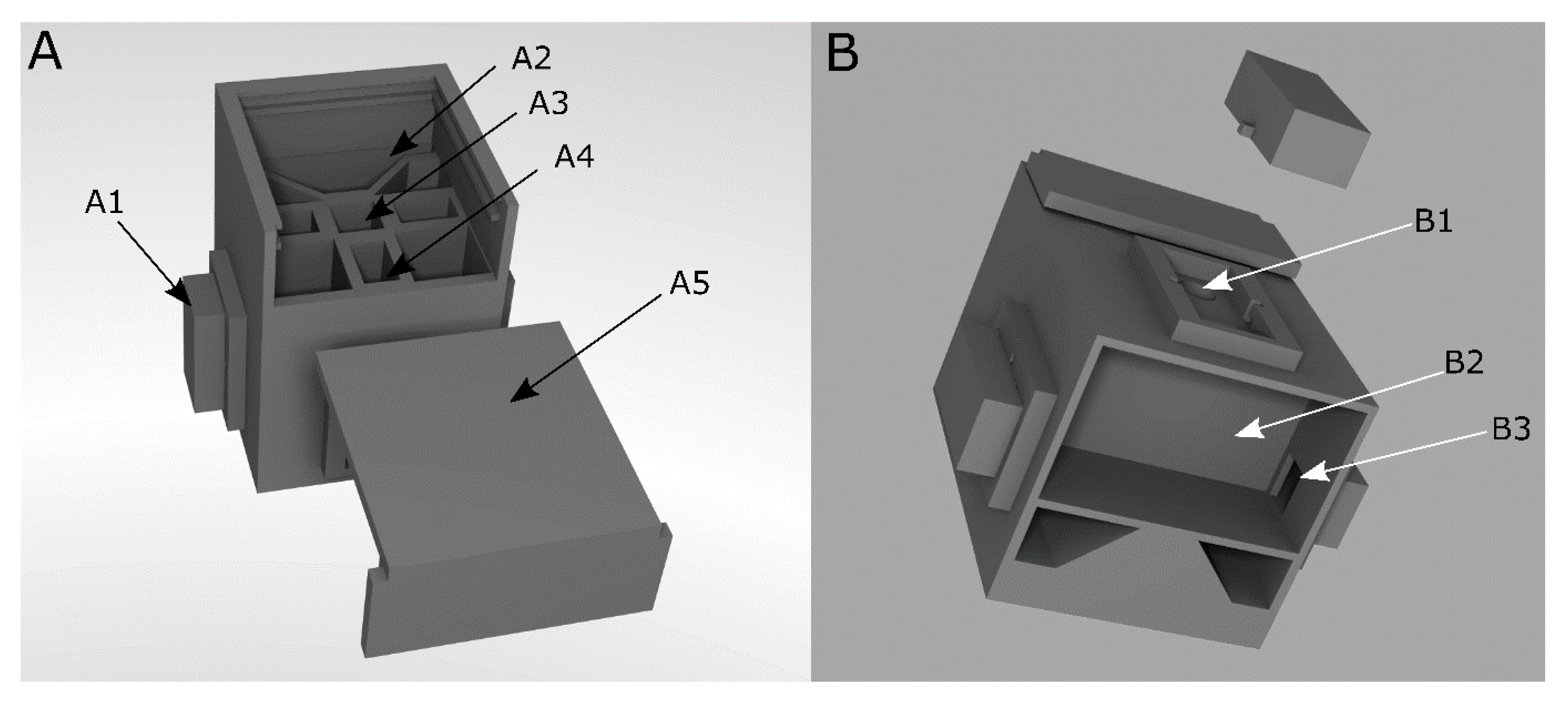
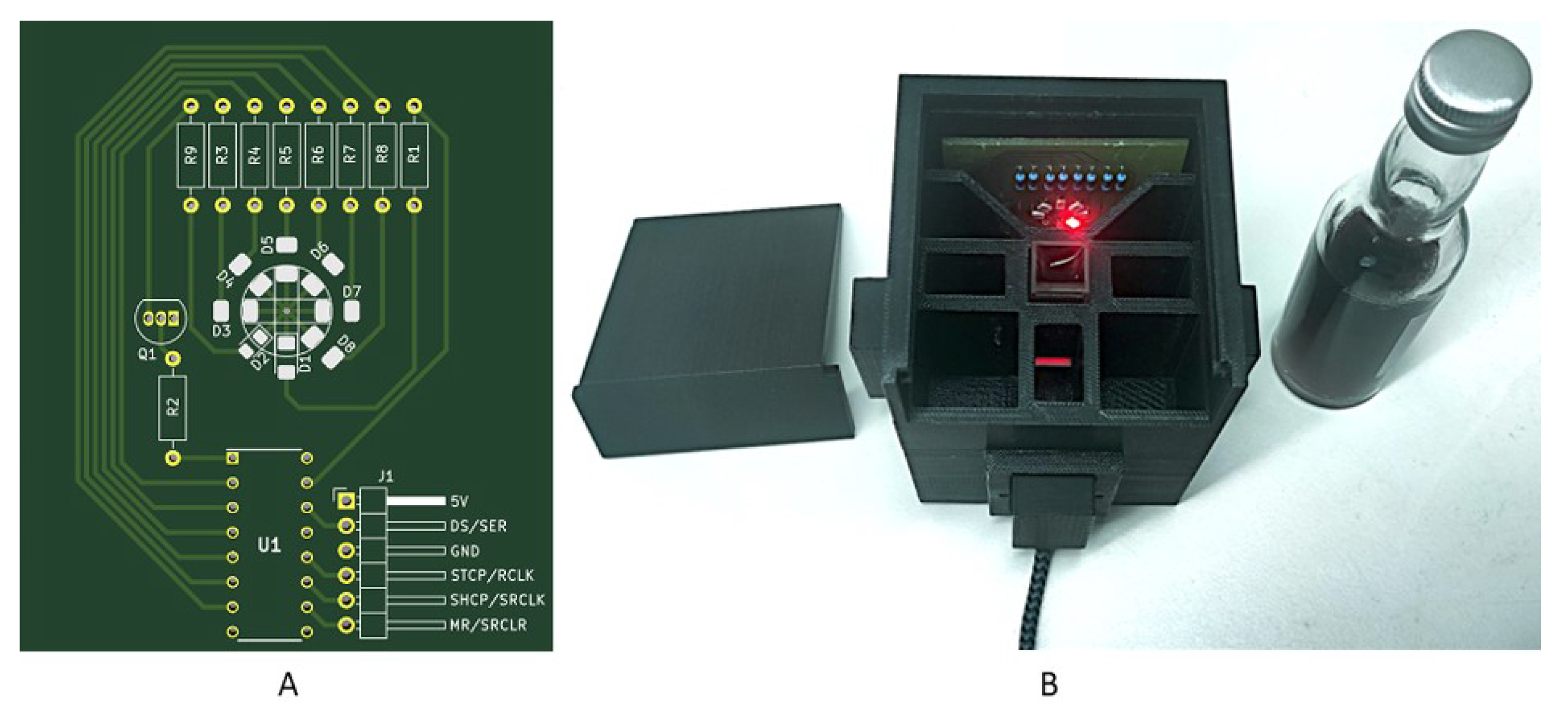
2.4. Portable Analysis System

2.4.1. Measurement Chamber

A portable analysis system, as described earlier [47], was used for transmission measurements to simplify the wine color determination. The measurement chamber (Figure 1) was 3D-printed in black acrylonitrile butadiene styrene (ABSplusTM, Stratasys GmbH, Frankfurt am Main, Germany). To avoid using optical filters or dispersing elements, LEDs of single wavelengths were integrated as the light source. Light was measured using a phototransistor. The measurement principle is based on the discharge of a capacitor by the photocurrent of the phototransistor, and the discharge time is correlated with light intensity and thus with the transmission of a sample. The in-detail description of the circuit was described earlier [47].

The LEDs and the phototransistor are placed in LED inserts by LED mounting clips (Figure 1(B1)). The circuit board is mounted in the bottom compartment of the measuring chamber (Figure 1(B2)).To perform transmission measurements, the LED is positioned opposite the light sensor. The sample is inserted into a cuvette in the middle of the measuring chamber between the light source and sensor. After the components and the sample has been inserted, the chamber is closed to avoid interference from ambient light (Figure 1(A1,A5)).

2.4.2. Data Recording

For interpolation of the transmission spectra of wine, LEDs with the required wavelengths were integrated into the system. An LED board with all required surface-mounted-device-LEDs (SMD-LEDs) was developed to avoid the installation and removal of LEDs during the measurement. The LEDs were controlled by the microcontroller via a shift register (Figure 2).

For 10 white wines and 10 red wines, measurement data obtained using the portable analysis system was correlated with corresponding transmission values from the laboratory photometer. This is important because of the varying sensitivity of the phototransistor at different wavelengths [48] and with this, the different correlations for the measured values with the portable analysis system and the laboratory photometer for different wavelengths. Subsequently, transmission values of the remaining white and red wines were calculated. Red wines were measured in a 4 mm glass cuvette, and white wines were measured in a 10 mm glass cuvette. Afterwards, the spectra of wine were interpolated, and CIE L*a*b* coordinates were calculated according to the OIV.

2.4.3. Data Processing of Single Wavelength Measurements to Retrieve CIE L*a*b* Coordinates

In one approach, transmission values at single wavelengths were used directly in the empirical formulae to predict the CIE L*a*b* coordinates. In another approach, the transmission spectra of wine samples were interpolated based on transmission values at single wavelengths. Completed spectra were then used to calculate CIE L*a*b* coordinates. To determine the accuracy of each method, ΔE was calculated between the predicted CIE L*a*b* coordinates and those calculated according to the OIV (Equation (4)).

$$\Delta E=\sqrt{{(L_{measured}^{*}-L_{predicted}^{*})}^2+{(a_{measured}^{*}-a_{predicted}^{*})}^2+{(b_{measured}^{*}-b_{predicted}^{*})}^2}$$

(4)

These investigations were performed for 56 red and 56 white wines. Spectra of all 112 wines were recorded on a double beam photometer (V-730, JASCO, Tokio, Japan) using a data interval of 1 nm in combination with a scan speed of 1000 nm/min.

Empirical Formulae to Calculate Wine Color

Two empirical formulae from Hardy et al. [42] and Ayala et al. [41] were compared. Both methods allow the calculation of CIE L*a*b* coordinates from transmission values at single wavelengths. Hardy et al. prescribed the balanced ordinates method, according to which the CIE XYZ color valances are calculated by four transmission values at 445 nm, 495 nm, 550 nm and 625 nm. These calculated color coordinates are related to the standard illuminant C and the 2°-standard observer as reference points. The method published by Ayala et al. is based on characteristic vector analysis, where CIE XYZ color valences are calculated from three transmission measurements at 440 nm, 530 nm and 600 nm. These color coordinates are related to the D65 standard illuminant, the 10°-standard observer, and a 2 mm path length. Both methods calculate the CIE XYZ color valances, which can be used to determine the CIE L*a*b coordinates [12].

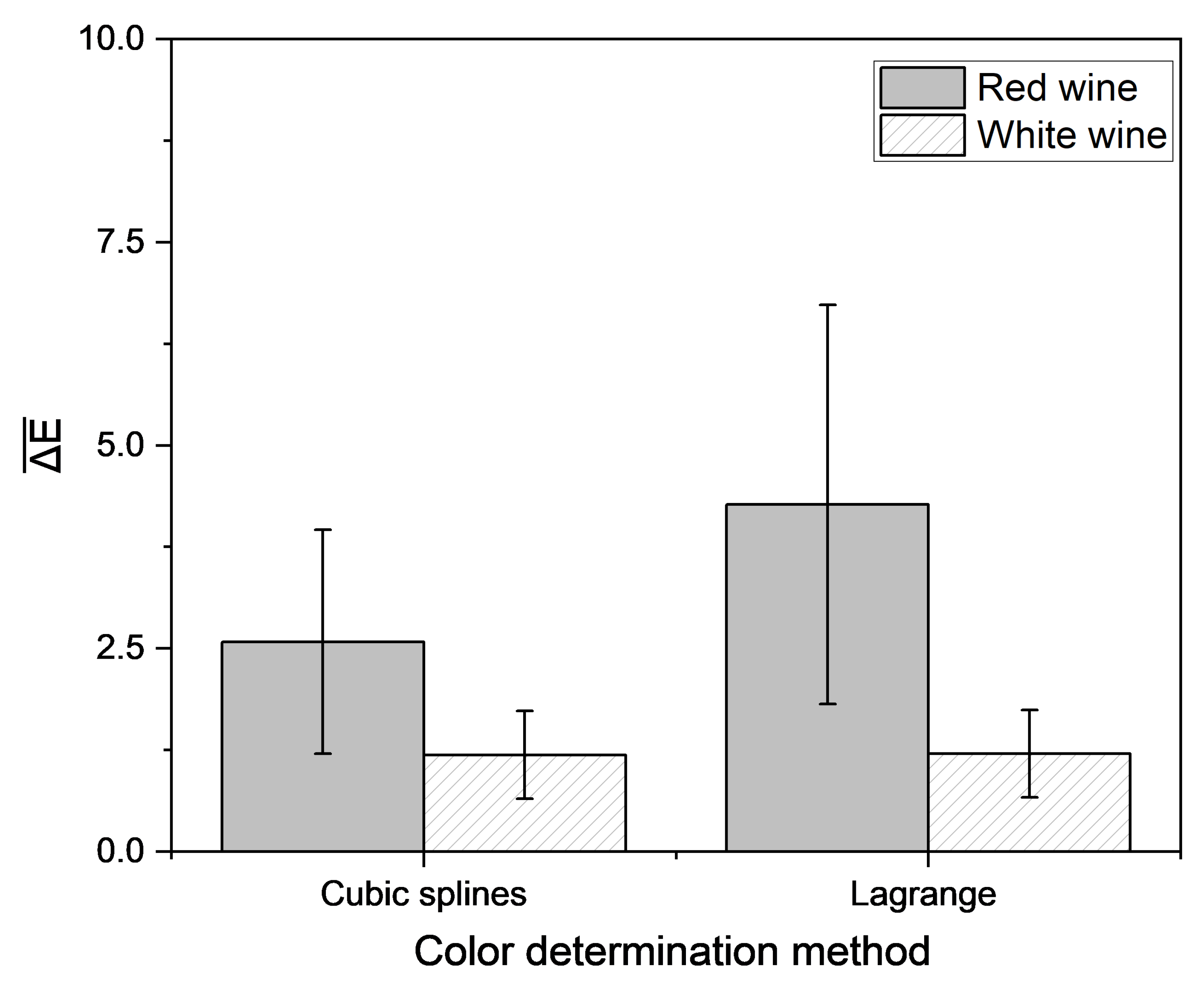
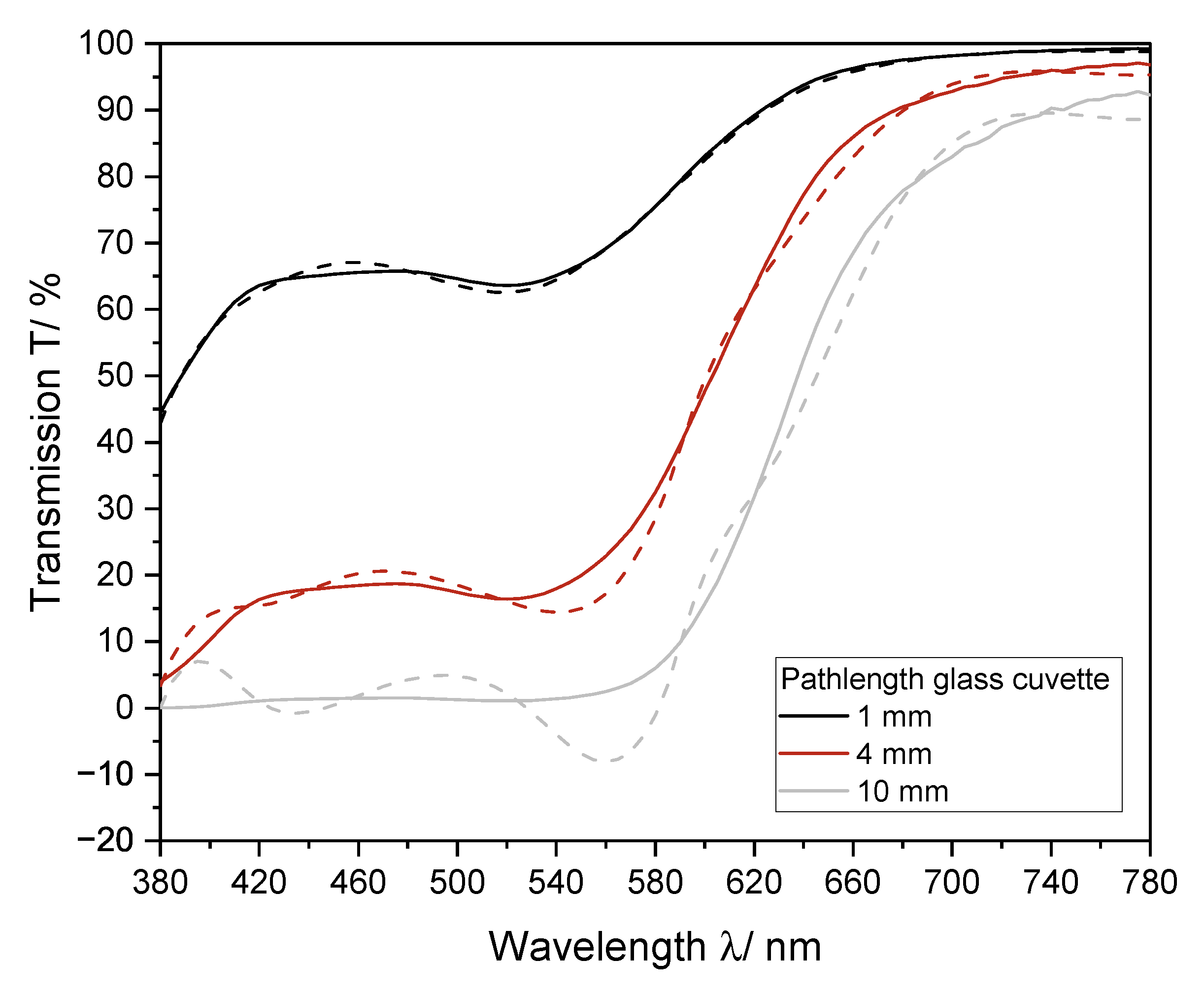
Interpolation Methods

Three different interpolation methods were compared to generate complete transmission spectra subsequently used to calculate CIE L*a*b* coordinates. Interpolation according to Lagrange [49] delivers a polynomial with a degree of n − 1, where n is the number of supporting points. With the interpolation according to Sprague [50], polynomials of the fifth degree are calculated to describe the course of a function between two supporting points. Consequently, n − 1 polynomials are required to describe the function between n supporting points. For the calculation of the coefficients, data from outside the data set is needed, thus extrapolation of data is necessary. The interpolation with cubic splines [51] yields n − 1 polynomials of third grade. Like the interpolation according to Sprague, the function between two supporting points is described by this polynomial. For interpolation with cubic splines, two assumptions must be made due to double overdetermination of the equation system. In this case, the first derivation at the upper and lower bounds of reconstructed spectra were set to one for 380 nm and zero for 780 nm.

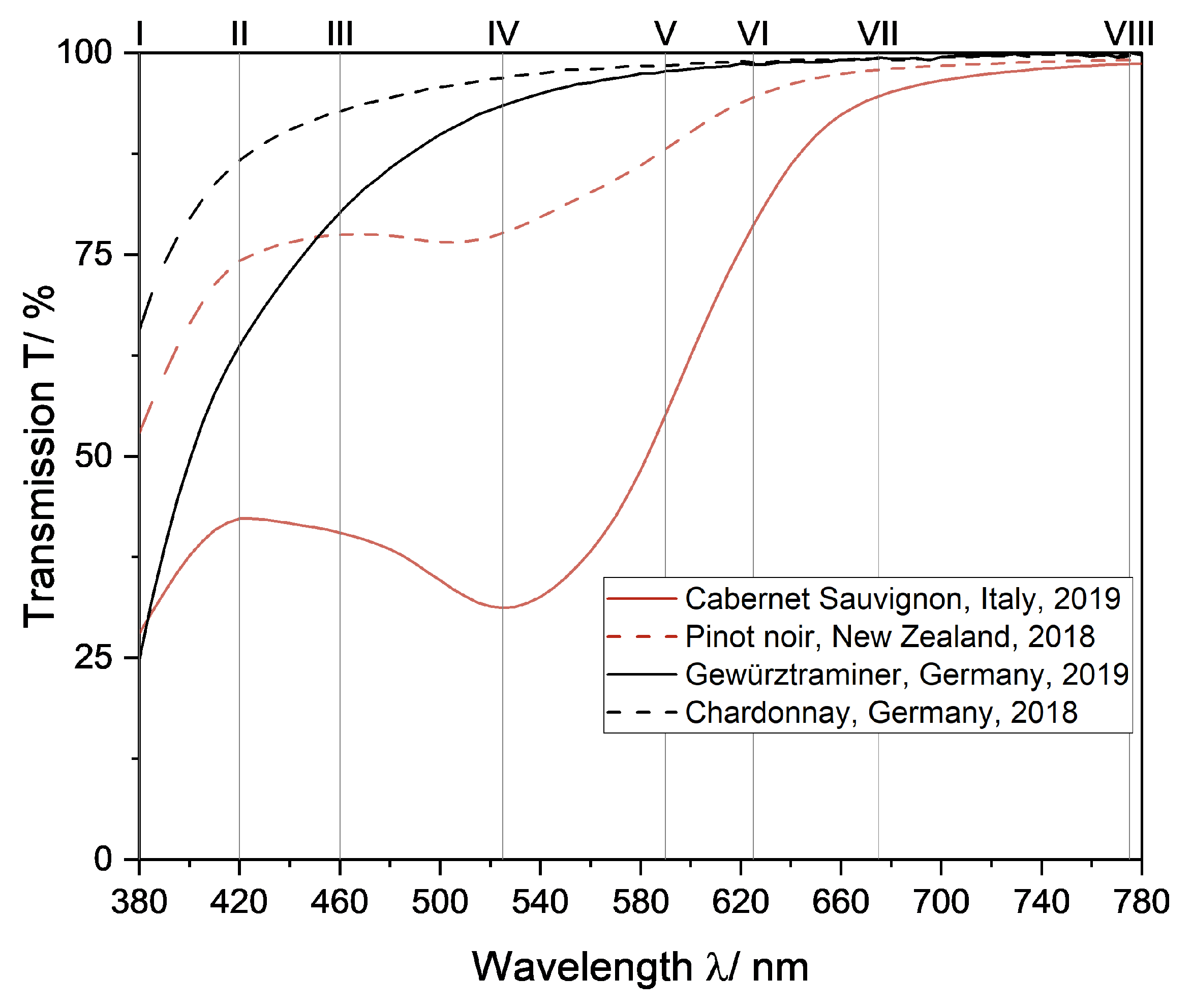
Selection of Supporting Points for Interpolation

Eight supporting points were chosen at extreme points, inflection points, and other points of interest in the transmission spectra of red and white wine (Figure 3) for interpolation.

The transmission spectra from red wine show a local maximum in the range of 400–440 nm, an inflection point in the range of 440–510 nm, a local minimum in the range of 510–560 nm, an inflection point in the range of 560–620 nm and a plateau in the range of 620–650 nm. To ensure the spectra were interpolated correctly between these ranges, supporting points were selected in these regions. Therefore, considering the commercial availability of LEDs, the transmission of wine samples was measured at the wavelengths 420 nm, 525 nm, 560 nm and 625 nm (

Table 1. Supporting points chosen in transmission spectra for color determination of red and white wine based on interpolation methods. Supporting points were chosen based on transmission spectra of red wine (Figure 3(I–VIII)).

Number	Region	Wavelength Region	Wavelength of Commercially Available LED
I	Lower bound ultraviolet region	380 nm	380 nm
II	Local maximum	400–440 nm	420 nm
III	Gap filler 1	440–510 nm	460 nm
IV	Local minimum	510–560 nm	525 nm
Î V	Gap filler 1	560–620 nm	590 nm
VI	Strong increasing slope	620–650 nm	625 nm
VII	Gap filler 1	650–775 nm	675 nm
VIII	Edge infrared region	780 nm	775 nm

¹ Gap fillers to bridge areas in transmission spectra.

II, IV, V and VI). Because the distance between supporting point VI and the end of the spectrum is quite large and would likely cause errors, an additional supporting point was added in this range for greater accuracy of interpolated spectra (Table 1, VII). Lastly, supporting points at the upper and lower bounds of the transmission spectra were chosen, since the slope here varied from wine to wine (Figure 3 and Table 1, I and VIII). No additional LED was chosen between VII and VIII because the transmission in this region does not change from stable without any further points of interest.

2.5. Statistical Analysis

Calculations using the empirical methods and Lagrange interpolation were conducted in Excel (Microsoft, Redmond, WA, USA). Cubic splines and Sprague interpolation were implemented in MATLAB (R2020b, MathWorks, USA). To evaluate the normal distribution of data, the Shapiro-Wilk test was conducted in Origin (Pro) (2020b, OriginLab, USA), where H₀ states that the data follows a normal distribution. To verify significance of the results, an ANOVA, where the H₀ is accepted if there are no differences between the mean values of the observed factor, was conducted in combination with Tukey’s HSD post hoc test. Here, the H₀ states that two observed means are equal. Both tests were also conducted in Origin(Pro) (2020b, OriginLab, USA). XLSTAT (2020, ADDINSOFT, France) was used for Bartlett’s test to verify the significance between variances. H₀ is accepted, if the variances are equal. Correlation matrices depicting Spearman coefficients were programmed in Python using the pandas [52], numpy [53], matplotlib [54] and seaborn [55] libraries.

3. Results and Discussion

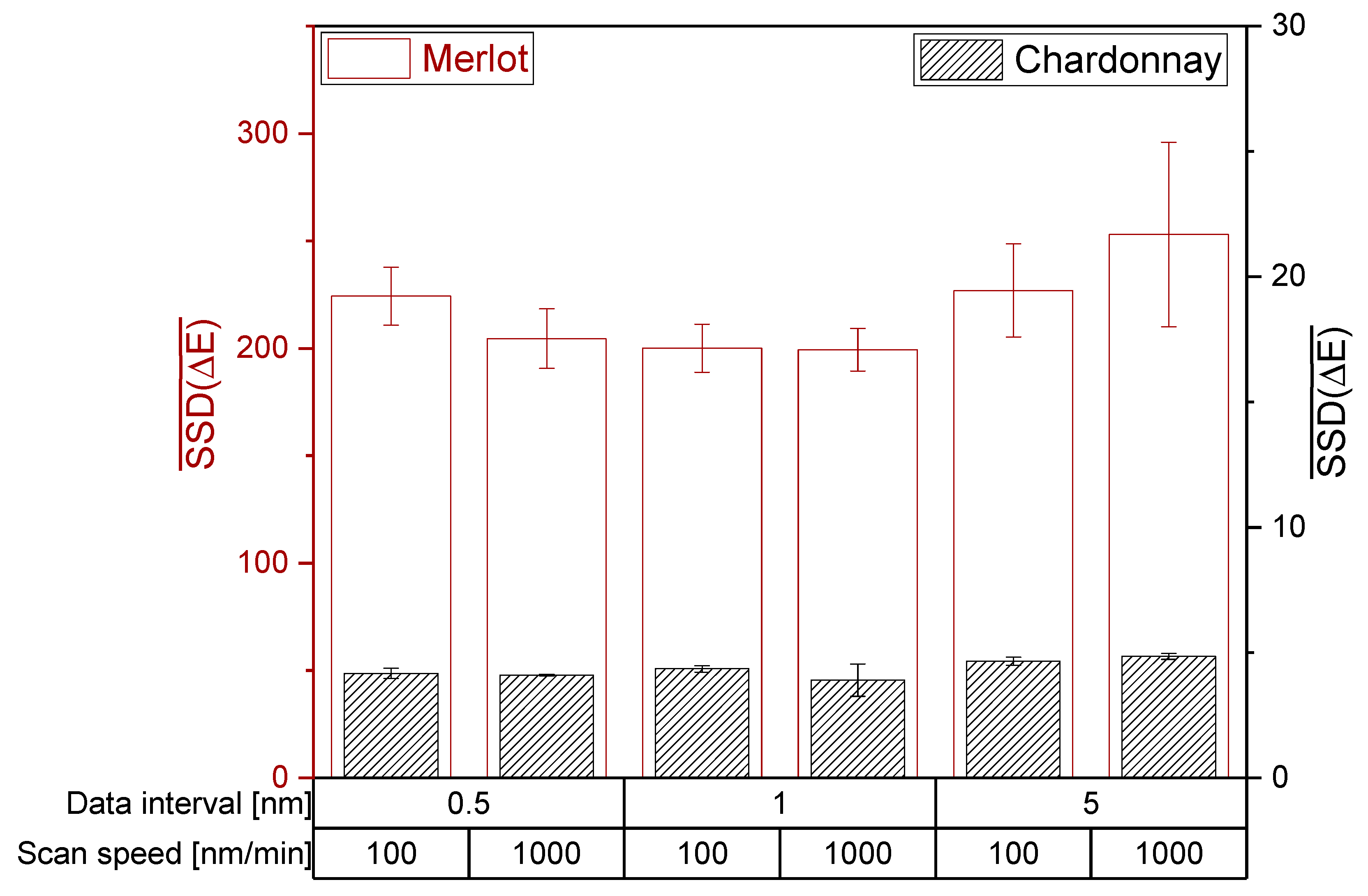
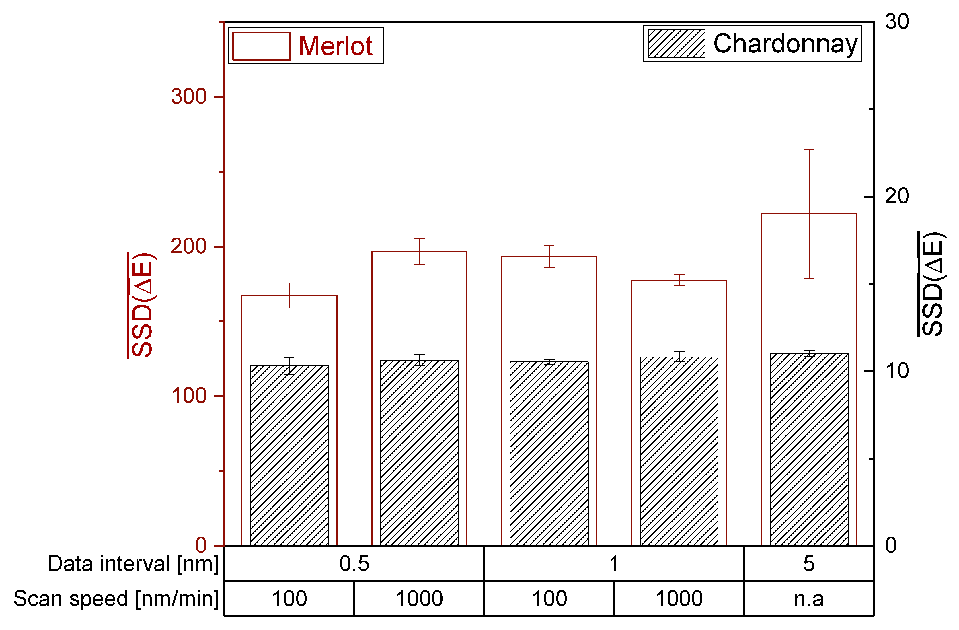
3.1. Influence of Photometer Settings on the Ability to Distinguish Wines and to Obtain Reproducible CIE L*a*b* Coordinates

For both photometers, H₀ of the ANOVA and Tukey HSD test is accepted and therefore the setting of the data interval and scan speed did not significantly affect the mean SSD (ΔE). Regarding Bartlett’s test, H₀ is rejected and the photometer settings have a significant impact on the variances of SSD(ΔE). Hence, the investigated photometer settings did not affect the ability to distinguish wines by the CIE L*a*b* coordinates of red and white wines (Figure 4 and Figure 5). However, a high data interval of 5 nm in red wine resulted in the lowest reproducibility. Accordingly, data intervals lower than 5 nm are recommended for the CIE L*a*b* measurement of red wines.

The investigation of data interval and scan speed on different photometers revealed similar mean SSD(ΔE) for red wines, but not for white wines. The different mean SSD(ΔE) between the photometers suggest that different devices have different sensitivities in their detector systems in the limit of detection area, as demonstrated for white wine with unsaturated color. For red wines, the mean sum of squared deviations showed only differences for an extremely low data interval of 0.5 nm. Depending on the machine and its detector system, an extremely low data interval could lead to increased noise, consequently reducing the ability to distinguish the wine color. Therefore, a data interval higher than 0.5 nm is recommended.

For red wines, the mean sum of squared deviations showed only differences for an extremely low data interval of 0.5 nm. Depending on the machine and its detector system, an extremely low data interval could lead to increased noise, consequently reducing the ability to distinguish the wine color. Therefore, a data interval higher than 0.5 nm is recommended.

As for the scan speed, no differences between 100 and 1000 nm/min could be observed. Overall, data recording with 1 nm data interval and the faster scan speed of 1000 nm/min is suggested to obtain the best results for CIE L*a*b* coordinates.

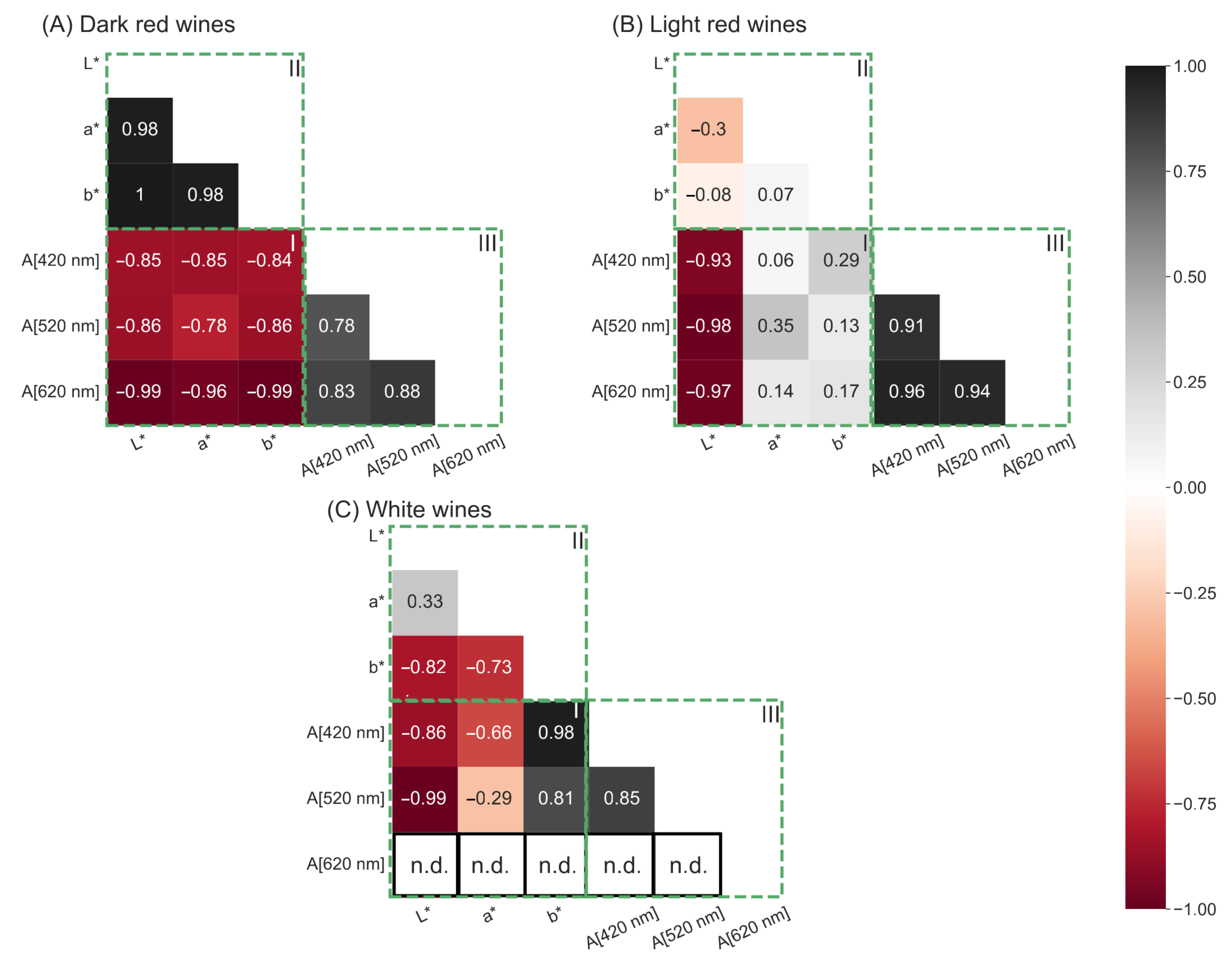
3.2. Correlation between CIE L*a*b* and Glories Method

After determining the specific photometer settings that yield reproducible CIE L*a*b* coordinates, the spectra of 56 red wines and 56 white wines were recorded to examine whether the CIE L*a*b* coordinates are comparable to Glories absorbance values. A good comparability between the two methods would prefer the Glories method over the CIE L*a*b* color space, since the Glories method does not require a complete transmission spectrum. The measured CIE L*a*b* coordinates and Glories parameters were correlated in a correlation matrix displaying the Spearman coefficient. For dark red wine, the CIE L*a*b* coordinates and Glories absorbance values show a strong negative correlation (Figure 6A(I)). Additionally, the L*a*b* coordinates correlate positively with itself (Figure 6A(II)) as well as the Glories absorbance values at wavelengths 420 nm, 520 nm and 620 nm (Figure 6A(III)).

A different observation was made for light red wine (Figure 6B). The coefficients in Figure 6B(I) are very low, indicating a weak correlation between the CIE L*a*b* coordinates and the Glories absorbance values. Furthermore, a weak correlation between the L*-, a*-, and b* coordinates was observed (Figure 6B(II)), while the Glories absorbance values demonstrate a strong positive correlation with each other (Figure 6B(III)).

Visualizing the Spearman coefficients for white wine, a strong negative correlation between the L* and b* coordinates and the Glories absorbance values was observed (Figure 6C(I)). However, the a*coordinate showed a weak correlation with all three Glories absorbance values (Figure 6C(I)). In white wine, the L*, and the b* coordinate correlated positively with each other (Figure 6C(II)). Furthermore, the a*, and the b* coordinate correlated positively with each other, but not the L* and a* coordinate (Figure 6C(II)). The Glories absorbance values, correlated well with each other (Figure 6C(III)). However, in white wine the absorbance at 620 nm was under the photometric accuracy and therefore could not be used in the correlation (Figure 6C(III)).

The observations demonstrate that the Glories and the CIE L*a*b* method can be used interchangeably for dark red wine, but not for white wine and light red wine. The Glories absorbance values in dark red, light red, and white wines correlated strongly among themselves, indicating a violation of Grassmann’s first law, which states that three independent parameters are needed to completely describe color. In dark red wines, the CIE L*a*b* coordinates correlate with each other as well, but since this is not the case in white wines and light red wines, it could be argued that the CIE L*a*b* coordinates are more independent than the Glories absorbance values. Therefore, the CIE L*a*b* color space is better suited for use in wine than color measurement, according to Glories.

Additionally, the Glories color measurement violates Grassmann’s first law in white wine because, without absorbance values at 620 nm, the remaining two absorbances at 420 and 520 nm cannot sufficiently describe color.

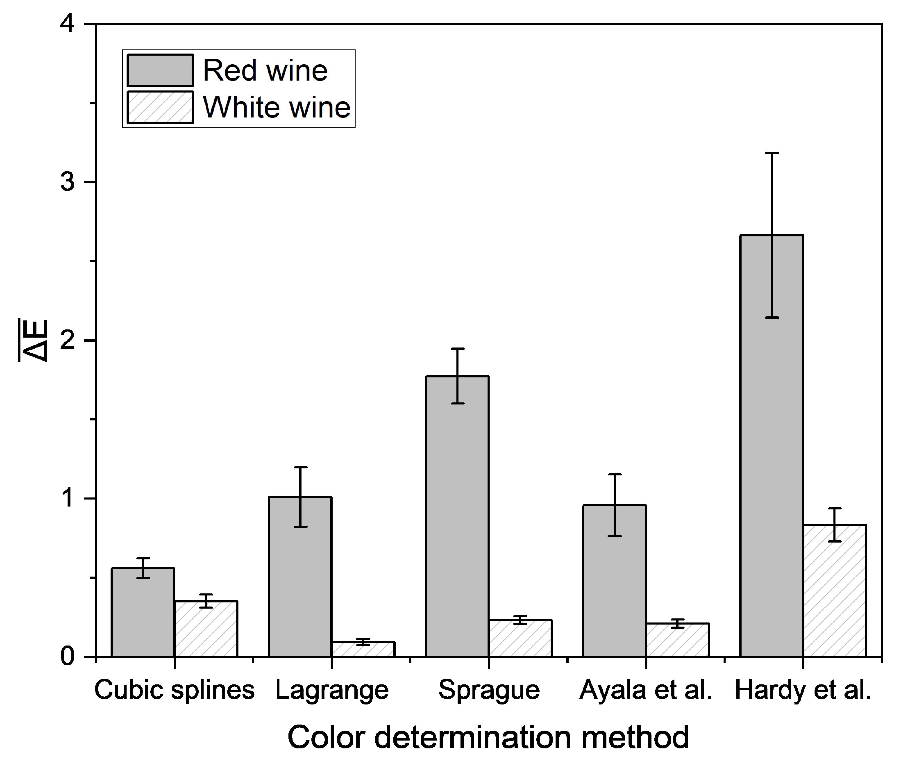
3.3. Simplification of Wine Color Measurement

Different empirical and interpolation methods were investigated to determine the color of wine using single wavelength transmission values measured using a laboratory photometer. For each wine, CIE L*a*b* coordinates were calculated from complete spectra and from spectra derived from single wavelength transmission values via empirical and interpolation methods. The accuracy of the derived CIE L*a*b* coordinates was determined by their ΔE in relation to the CIE L*a*b* coordinates calculated from the complete spectra (Figure 7).

For red wine, the lowest color difference between measured and predicted CIE L*a*b* coordinates was achieved using the interpolation via cubic splines. The method of Hardy et al. yielded the highest color difference for both red and white wine. Regardless of the method, the color difference for white wine was lower than for red wine. For white wine, using the method recommended by the OIV, the lowest deviation was attained by the interpolation of spectra according to Lagrange. In general, a color difference under 3 is not perceivable to the observer [56], but there are different data for the threshold value for visible color, ranging from 1 to 14 [57]. This suggests that differences between results obtained using these color determination methods and those from the official method of the OIV likely cannot be perceived by the observer, except for the method according to Hardy et al. for red wines. Therefore, the methods are suitable for the determination of wine color. Because the interpolation with cubic splines and interpolation according to Lagrange demonstrated the best results for red and white wine, these methods were integrated into the portable analysis system. The difference in color measured using this system and the color calculated using the OIV method was determined (Figure 8).

The Euclidean color distance determined by the portable analysis system was higher as compared to that determined by the laboratory photometer alone. To establish the interpolation methods, the required transmission values were extracted directly from the measured spectra. Therefore, the same data set was used for all color determination methods. For implementation into the portable analysis system, the measured data had to be correlated with the transmission at the laboratory photometer in an extra step to be suited for color determination. In contrast to the laboratory photometer, a 4 mm cuvette was used for the color calculation with the portable analysis system. It could be shown that the use of a cuvette with a longer pathlength leads to a greater deviation of the interpolated spectra from the spectra, recorded with the laboratory device (Figure 9). Therefore, an adapter for usage of 1 mm cuvette should be integrated.

The lowest Euclidean color distance, calculated with the portable analysis system from the color measured with the laboratory photometer for red wine resulted from interpolation with cubic splines, in agreement with the previously shown investigations. There is a total of 72% of the 46 red wines below ΔE of three. For white wine, all methods resulted in similar color differences, which were below a value of three. These findings indicate that wine color can be determined using a portable low-cost photometer by interpolation of transmission spectra, for the majority of the sample set closely approximating results from the laboratory photometer.

4. Conclusions

This study demonstrated the significant influence of the photometer settings data interval and scan speed on the reproducibility of measurements. The CIE L*a*b* coordinates were found to correlate with the Glories absorbance values in dark red wine (L* < 20), but not in white wine and light red wine (L* > 20). However, Glories absorbance values correlated with themselves in all three wine categories, which indicates a dependency between parameters in violation of Grassmann’s first law. The CIE L*a*b* color space is potentially more reliable for color calculation in wine, but further research is required to investigate which of the two systems correlate better with the human color perception. The calculation of CIE L*a*b* coordinates for wine color based on single wavelength measurements instead of complete transmission spectra is possible. The best results using a laboratory photometer were achieved using the cubic splines (for red wine) and Langrange (for white wine) methods of interpolation. Implementation of the portable analysis system resulted in a higher color difference between measured and predicted CIE L*a*b* coordinates. The determination of white wine color was more successful than in red wine. Furthermore, color determination could be improved using an adapter for a 1 mm cuvette in the portable analysis system. With this investigations, color inexpensive determination of wine is possible. The portable analysis system can be built with low-cost components for about 100€. In comparison to that, laboratory photometers are available from 1.000 to more than 10.000€ This color calculation is highly specialized on wine and cannot be performed with other matrices due to different maxima and minima throughout the spectra. Here, other supporting points are needed. Furthermore, color of sparkling wine or turbid samples cannot be determined due to light scattering. These samples have to be degassed or filtered. Therefore, these investigations could be focused on in future studies.

References

1. Peynaud, E.; Blouin, J. El Gusto del Vino: El gran Libro de la Degustación, 2a. ed., reimp ed.; Mundi-Prensa: Madrid, Spain, 2002. [Google Scholar]
2. Morrot, G.; Brochet, F.; Dubourdieu, D. The color of odors. Brain Lang. 2001, 79, 309–320. [Google Scholar] [CrossRef] [PubMed] [Green Version]
3. Grassmann. XXXVII. On the theory of compound colours. Lond. Edinb. Dublin Philos. Mag. J. Sci. 1854, 7, 254–264. [Google Scholar] [CrossRef]
4. Glories, Y. La couleur des vins rouges. lre partie: Les équilibres des anthocyanes et des tanins. OENO ONE 2016, 18, 195. [Google Scholar] [CrossRef] [Green Version]
5. Ribéreau-Gayon, P. Handbook of Enology: Volume 2: The Chemistry of Wine Stabilization and Treatments, 2nd ed.; John Wiley: Chichester/West Sussex, England, 2006. [Google Scholar]
6. ISO/CIE 11664-1:2019; Colorimetry—Part 1: CIE Standard Colorimetric Observers. DIN e.V.: Berlin, Germany, 2019.
7. DIN EN ISO/CIE 11664-2:2019; Colorimetry—Part 2: CIE Standard Illuminants. DIN e.V.: Berlin, Germany, 2011.
8. Wright, W.D. A re-determination of the trichromatic coefficients of the spectral colours. Trans. Opt. Soc. 1929, 30, 141–164. [Google Scholar] [CrossRef]
9. Wright, W.D. A re-determination of the mixture curves of the spectrum. Trans. Opt. Soc. 1930, 31, 201–218. [Google Scholar] [CrossRef]
10. Guild, J. The colorimetric properties of the spectrum. Philos. Trans. R. Soc. Lond. Ser. A Contain. Pap. Math. Phys. Character 1931, 230, 149–187. [Google Scholar] [CrossRef] [Green Version]
11. Stiles, W.S.; Burch, J.M. N.P.L. Colour-matching Investigation: Final Report (1958). Opt. Acta Int. J. Opt. 1959, 6, 1–26. [Google Scholar] [CrossRef]
12. DIN EN ISO/CIE 11664-4:2019; Colorimetry—Part 4: CIE 1976 L*a*b* Colour Space. DIN e.V.: Berlin, Germany, 2020.
13. DIN EN ISO/CIE 11664-6:2019; Colorimetry—Part 6: CIEDE2000 Colour-Difference Formula. DIN e.V.: Berlin, Germany, 2016.
14. Compendium of International Analysis of Methods-Method OIV-MA-AS2-11: Determination of Chromatic Characteristics According to CIELab; International Organisation of Wine and Vine: Paris, France, 2006; ISBN 978-2-85038-033-4.
15. Compendium of International Analysis of Methods-OIV Chromatic Characteristics-Method OIV-MA-AS2-07B: Determination of Chromatic Characteristics According to CIELab; International Organisation of Wine and Vine: Paris, France, 2006; ISBN 978-2-85038-033-4.
16. Pérez-Magariño, S.; González-Sanjosé, M.L. Application of absorbance values used in wineries for estimating CIELAB parameters in red wines. Food Chem. 2003, 81, 301–306. [Google Scholar] [CrossRef]
17. García-Marino, M.; Escudero-Gilete, M.L.; Heredia, F.J.; Escribano-Bailón, M.T.; Rivas-Gonzalo, J.C. Color-copigmentation study by tristimulus colorimetry (CIELAB) in red wines obtained from Tempranillo and Graciano varieties. Food Res. Int. 2013, 51, 123–131. [Google Scholar] [CrossRef] [Green Version]
18. Zhang, X.K.; Lan, Y.B.; Huang, Y.; Zhao, X.; Duan, C.Q. Targeted metabolomics of anthocyanin derivatives during prolonged wine aging: Evolution, color contribution and aging prediction. Food Chem. 2021, 339, 127795. [Google Scholar] [CrossRef]
19. Wang, L.J.; Naudé, N.; Chang, Y.C.; Crivaro, A.; Kamoun, M.; Wang, P.; Li, L. An ultra-low-cost smartphone octochannel spectrometer for mobile health diagnostics. J. Biophotonics 2018, 11, e201700382. [Google Scholar] [CrossRef] [PubMed]
20. Dutta, S.; Sarma, D.; Patel, A.; Nath, P. Dye-Assisted pH Sensing Using a Smartphone. IEEE Photonics Technol. Lett. 2015, 27, 2363–2366. [Google Scholar] [CrossRef]
21. Ju, Y.G. Fabrication of a low-cost and high-resolution papercraft smartphone spectrometer. Phys. Educ. 2020, 55, 035005. [Google Scholar] [CrossRef] [Green Version]
22. Kong, W.; Kuang, D.; Wen, Y.; Zhao, M.; Huang, J.; Yang, C. Solution Classification With Portable Smartphone-Based Spectrometer System Under Variant Shooting Conditions by Using Convolutional Neural Network. IEEE Sens. J. 2020, 20, 8789–8796. [Google Scholar] [CrossRef]
23. Jian, D.; Wang, B.; Huang, H.; Meng, X.; Liu, C.; Xue, L.; Liu, F.; Wang, S. Sunlight based handheld smartphone spectrometer. Biosens. Bioelectron. 2019, 143, 111632. [Google Scholar] [CrossRef]
24. Zhang, C.; Cheng, G.; Edwards, P.; Zhou, M.D.; Zheng, S.; Liu, Z. G-Fresnel smartphone spectrometer. Lab Chip 2016, 16, 246–250. [Google Scholar] [CrossRef]
25. Edwards, P.; Zhang, C.; Zhang, B.; Hong, X.; Nagarajan, V.K.; Yu, B.; Liu, Z. Smartphone based optical spectrometer for diffusive reflectance spectroscopic measurement of hemoglobin. Sci. Rep. 2017, 7, 12224. [Google Scholar] [CrossRef] [Green Version]
26. Maity, M.; Gantait, K.; Mukherjee, A.; Chatterjee, J. Visible Spectrum-based Classification of Malaria Blood Samples on Handheld Spectrometer. In Proceedings of the 2019 IEEE International Instrumentation and Measurement Technology Conference (I2MTC), Auckland, New Zealand, 20–23 May 2019; IEEE: New York, NY, USA, 2019; pp. 1–5. [Google Scholar] [CrossRef]
27. Wilkes, T.C.; Pering, T.D.; McGonigle, A.J.S.; Willmott, J.R.; Bryant, R.; Smalley, A.L.; Mims, F.M.; Parisi, A.V.; England, R.A. The PiSpec: A Low-Cost, 3D-Printed Spectrometer for Measuring Volcanic SO2 Emission Rates. Front. Earth Sci. 2019, 7. [Google Scholar] [CrossRef]
28. Wilkes, T.C.; McGonigle, A.J.S.; Willmott, J.R.; Pering, T.D.; Cook, J.M. Low-cost 3D printed 1 nm resolution smartphone sensor-based spectrometer: Instrument design and application in ultraviolet spectroscopy. Opt. Lett. 2017, 42, 4323–4326. [Google Scholar] [CrossRef]
29. Albert, D.R.; Todt, M.A.; Davis, H.F. A Low-Cost Quantitative Absorption Spectrophotometer. J. Chem. Educ. 2012, 89, 1432–1435. [Google Scholar] [CrossRef]
30. Long, K.D.; Woodburn, E.V.; Le, H.M.; Shah, U.K.; Lumetta, S.S.; Cunningham, B.T. Multimode smartphone biosensing: The transmission, reflection, and intensity spectral (TRI)-analyzer. Lab Chip 2017, 17, 3246–3257. [Google Scholar] [CrossRef] [PubMed]
31. Zhao, R.A.; Shen, T.; Lang, T.; Cao, B. Visible smartphone spectrometer based on the transmission grating. In Proceedings of the 2017 16th International Conference on Optical Communications and Networks (ICOCN), Wuzhen, China, 7–10 August 2017; pp. 1–3. [Google Scholar] [CrossRef]
32. Plaipichit, S.; Wicharn, S.; Buranasiri, P. Spectroscopy system using digital camera as two dimensional detectors for undergraduate student laboratory. Mater. Today Proc. 2018, 5, 11114–11122. [Google Scholar] [CrossRef]
33. Ding, H.; Chen, C.; Qi, S.; Han, C.; Yue, C. Smartphone-based spectrometer with high spectral accuracy for mHealth application. Sens. Actuators A Phys. 2018, 274, 94–100. [Google Scholar] [CrossRef]
34. Woodburn, E.V.; Long, K.D.; Cunningham, B.T. Analysis of Paper-Based Colorimetric Assays with a Smartphone Spectrometer. IEEE Sens. J. 2019, 19, 508–514. [Google Scholar] [CrossRef] [PubMed]
35. Gallegos, D.; Long, K.D.; Yu, H.; Clark, P.P.; Lin, Y.; George, S.; Nath, P.; Cunningham, B.T. Label-free biodetection using a smartphone. Lab Chip 2013, 13, 2124–2132. [Google Scholar] [CrossRef]
36. Liu, L.; Bi, H. Utilising Smartphone Light Sensors to Measure Egg White Ovalbumin Concentration in Eggs Collected from Yinchuan City, China. J. Chem. 2020, 2020, 1–8. [Google Scholar] [CrossRef]
37. Cesar Souza Machado, C.; Da Silveira Petruci, J.F.; Silva, S.G. An IoT optical sensor for photometric determination of oxalate in infusions. Microchem. J. 2021, 168, 106466. [Google Scholar] [CrossRef]
38. Khoshmaram, L.; Mohammadi, M.; Nazemi Babadi, A. A portable low-cost fluorimeter based on LEDs and a smart phone. Microchem. J. 2021, 171, 106773. [Google Scholar] [CrossRef]
39. Valenzuela, I.C.; Cruz, F.R.G. (Eds.) Opto-Electric Characterization of pH Test Strip Based on Optical Absorbance Using Tri-Chromatic LED and Phototransistor; IEEE: New York, NY, USA, 2015. [Google Scholar]
40. Negueruela, A.I.; Echávarri, J.F.; Pérez, M.M. A Study of Correlation Between Enological Colorimetric Indexes and CIE Colorimetric Parameters in Red Wines. Am. J. Enol. Vitic. 1995, 353–356. [Google Scholar]
41. Ayala, F.; Echávarri, J.F.; Negueruela, A.I. A New Simplified Method for Measuring the Color of Wines. Am. J. Enol. Vitic. 1997, 48, 359–369. [Google Scholar]
42. Hardy, A.C. Handbook of Colorimetry, 4. auflage ed.; M.I.T. Press: Cambridge, MA, USA, 1966. [Google Scholar]
43. U.S. Bureau of Labor Statistics. CPI Average Price Data, U.S. City Average (AP); U.S. Bureau of Labor Statistics: Washington, DC, USA, 2022.
44. Australian Government. Priority 1: Increasing Demand and the Premium Paid for All Australien Wine; Australian Government: Canberra, Australia, 2020.
45. OIV. The State of Vitiviniculture; OIV: Paris, France, 2020. [Google Scholar]
46. Anderson, K.; Nelgen, S. Database of Regional, National and Global Winegrape Bearing Areas by Variety, 1960 to 2016. Available online: https://economics.adelaide.edu.au/wine-economics/databases#database-of-regional-national-and-global-winegrape-bearing-areas-by-variety-1960-to-2016 (accessed on 2 September 2020).
47. Di Nonno, S.; Ulber, R. Portuino-A Novel Portable Low-Cost Arduino-Based Photo- and Fluorimeter. Sensors 2022, 22, 7916. [Google Scholar] [CrossRef] [PubMed]
48. Mouser electronics Inc. Phototransistor SFH300. Available online: https://www.mouser.de/ProductDetail/OSRAM-Opto-Semiconductors/SFH-300-FA-3-4/?qs=K5ta8V%252BWhtZU3h4ylF8ddQ==&gclid=EAIaIQobChMI5Zn5r_Hc7gIVleh3Ch2TngduEAAYASAAEgJ1w_D_BwE (accessed on 13 December 2022).
49. Dahmen, W.; Reusken, A. Numerik für Ingenieure und Naturwissenschaftler, 2008th ed.; Springer: Berlin/Heidelberg, Germany, 2008. [Google Scholar]
50. de Kerf, J.L. The interpolation method of Sprague-Karup. J. Comput. Appl. Math. 1975, 1, 101–110. [Google Scholar] [CrossRef] [Green Version]
51. Colorimetry, 3rd ed.; CIE Technical Report; Commission Internationale de l’Eclairage: Vienna, Austria, 2004; Volume 15.
52. Reback, J.; McKinney, W.; Jbrockmendel; den Bossche, J.V.; Augspurger, T.; Cloud, P.; Gfyoung; Sinhrks; Klein, A.; Roeschke, M.; et al. pandas-dev/pandas: Pandas 1.0.3. 2020; Available online: https://zenodo.org/record/3715232#.Y5k4TX1BxPY (accessed on 5 November 2022).
53. Harris, C.R.; Millman, K.J.; van der Walt, S.J.; Gommers, R.; Virtanen, P.; Cournapeau, D.; Wieser, E.; Taylor, J.; Berg, S.; Smith, N.J.; et al. Array programming with NumPy. Nature 2020, 585, 357–362. [Google Scholar] [CrossRef] [PubMed]
54. Hunter, J.D. Matplotlib: A 2D graphics environment. Comput. Sci. Eng. 2007, 9, 90–95. [Google Scholar] [CrossRef]
55. Waskom, M. seaborn: Statistical data visualization. J. Open Source Softw. 2021, 6, 3021. [Google Scholar] [CrossRef]
56. Martínez, J.A.; Melgosa, M.; Pérez, M.M.; Hita, E.; Negueruela, A.I. Note. Visual and Instrumental Color Evaluation in Red Wines. Food Sci. Technol. Int. 2001, 7, 439–444. [Google Scholar] [CrossRef]
57. HEREDIA, F.J.; GUZMÁN-CHOZAS, M. The color of wine: A historical perspective, II. trichromatic methods. J. Food Qual. 1993, 16, 439–449. [Google Scholar] [CrossRef]
Figure 1. CAD model of the measurement chamber of the portable analysis system. (A): Front view. (B): Bottom view. A1: Lid to cover inserted LEDs and phototransistor, A2: Socket for SMD-LED board. A3: Place for a 10 mm-cuvette, A4: light path from LED to phototransistor, A5: Cover for the measuring chamber, B1: Place for LED or phototransistor B2: Bottom compartment for storage of a microcontroller and the circuit board, and B3: Path for cables to connect inserted LED and phototransistor [47].
Processes 10 02707 g001
Figure 2. (A) Developed LED board for color measurement with the portable analysis system. Eight SMD-LEDs with the needed wavelengths (Table 1) were placed in a circle (D1–D4). The required series resistors were connected (R1–R9). The LEDs were controlled by a shift register (U1). The board was developed in KiCAD (KiCAD version 5.1.9, Jean Pierre Charras, France). The LED board can be placed into the portable analysis system (B).
Processes 10 02707 g002
Figure 3. Transmission spectra of two red wines and two white wines to illustrate the choice of supporting points for color determination based on interpolation of transmission spectra. The position of supporting points is marked by numbers (I—VIII, Table 1).
Processes 10 02707 g003
Figure 4. Influence of the photometer settings data interval and scan speed on the CIE L*a*b* coordinates on the JASCO V-730 double beam photometer. The mean sum of squared deviations are shown with error bars (SD; n = 3; α = 0.05).
Processes 10 02707 g004
Figure 5. Influence of the photometer settings data interval and scan speed on the CIE L*a*b* coordinates on the Varian Cary 100 double beam photometer. The mean sum of squared deviation is shown with error bars (SD; n = 3; α = 0.05).
Processes 10 02707 g005
Figure 6. Correlation matrices depicting the Spearman coefficients for dark red wine ((A), n = 34), light red wine ((B), n = 22), and white wine ((C), n = 56). Evaluated were the correlations between CIE L*a*b* coordinates and Glories absorbance values at wavelengths 420 nm, 520 nm and 620 nm (A[420 nm], A[520 nm], A[620 nm]) (I), between L*, a*, and b* coordinates (II), and between Glories absorbance values (III).
Processes 10 02707 g006
Figure 7. Mean Euclidean color distance in the CIE L*a*b* color space based on different empirical methods and the reconstructed transmission spectra, determined by different interpolation approaches compared with the color determination method according to OIV [51]. Transmission data were measured with a laboratory photometer. Mean and 95% confidence interval of 56 red and 56 white wines are shown.
Processes 10 02707 g007
Figure 8. Mean Euclidean color distance in the CIE L*a*b* color space based on different empirical methods and the reconstructed transmission spectra, determined by different interpolation approaches compared with the color determination method according to OIV [51]. Transmission data were measured with a portable photometer and compared to data measured with the laboratory photometer. Mean and 95% confidence interval of 46 red and 46 white wines are shown.
Processes 10 02707 g008
Figure 9. Influence of pathlength of the cuvette on the interpolation of the transmission spectrum via cubic splines for a red wine. Measured was a Pinot Noir (2019) from Germany. The measured spectrum (solid line) and the interpolated spectrum (dashed line) for different pathlengths of glass cuvettes are shown. The spectrum was recorded with a 1 mm, 4 mm, and 10 mm glass cuvette.
Processes 10 02707 g009