
Study of the Dynamic Behavior of an Autonomous Inflow-Control Device Using a Digital Twin

 ,
,  and
and
Abstract
:1. Introduction
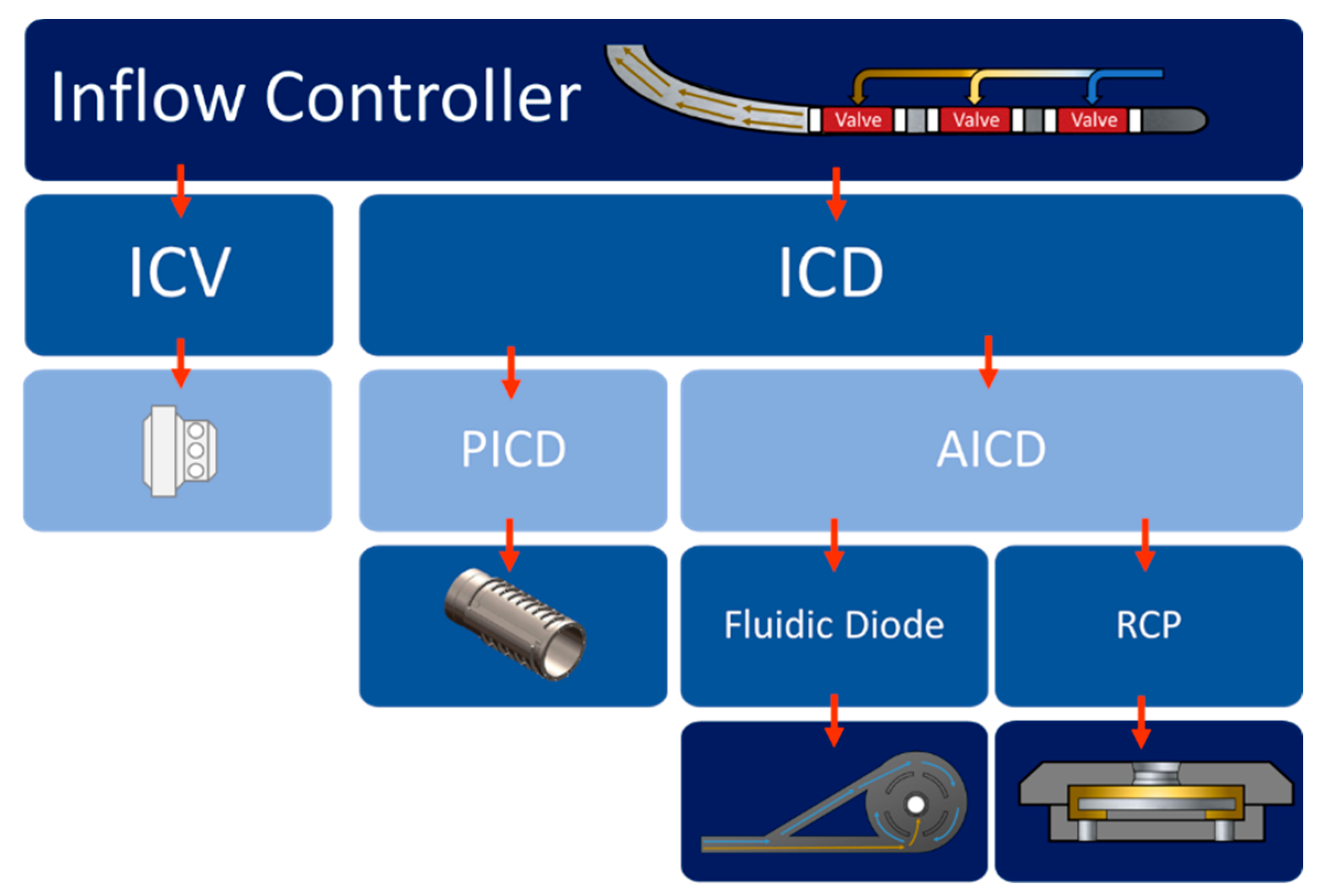
1.1. Inflow Controller Classification
1.2. Previous Works
1.3. CFD Governing Equations
1.3.1. Continuity Equation
1.3.2. Momentum Equation
1.3.3. Turbulence Equation
1.3.4. DFBI Equation
2. Materials and Methods
2.1. Valve Geometry and Experimental Data
2.2. Creation and Validation of the Numerical Model
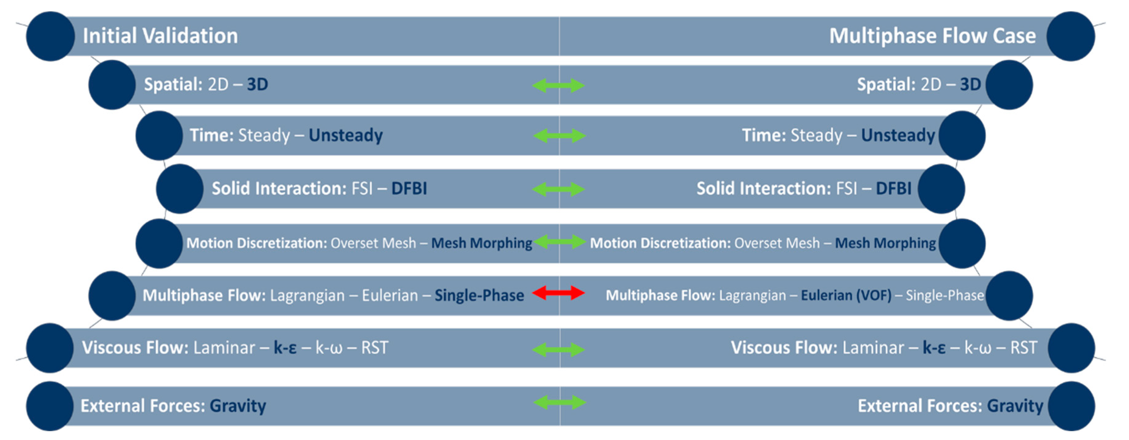
2.2.1. Models
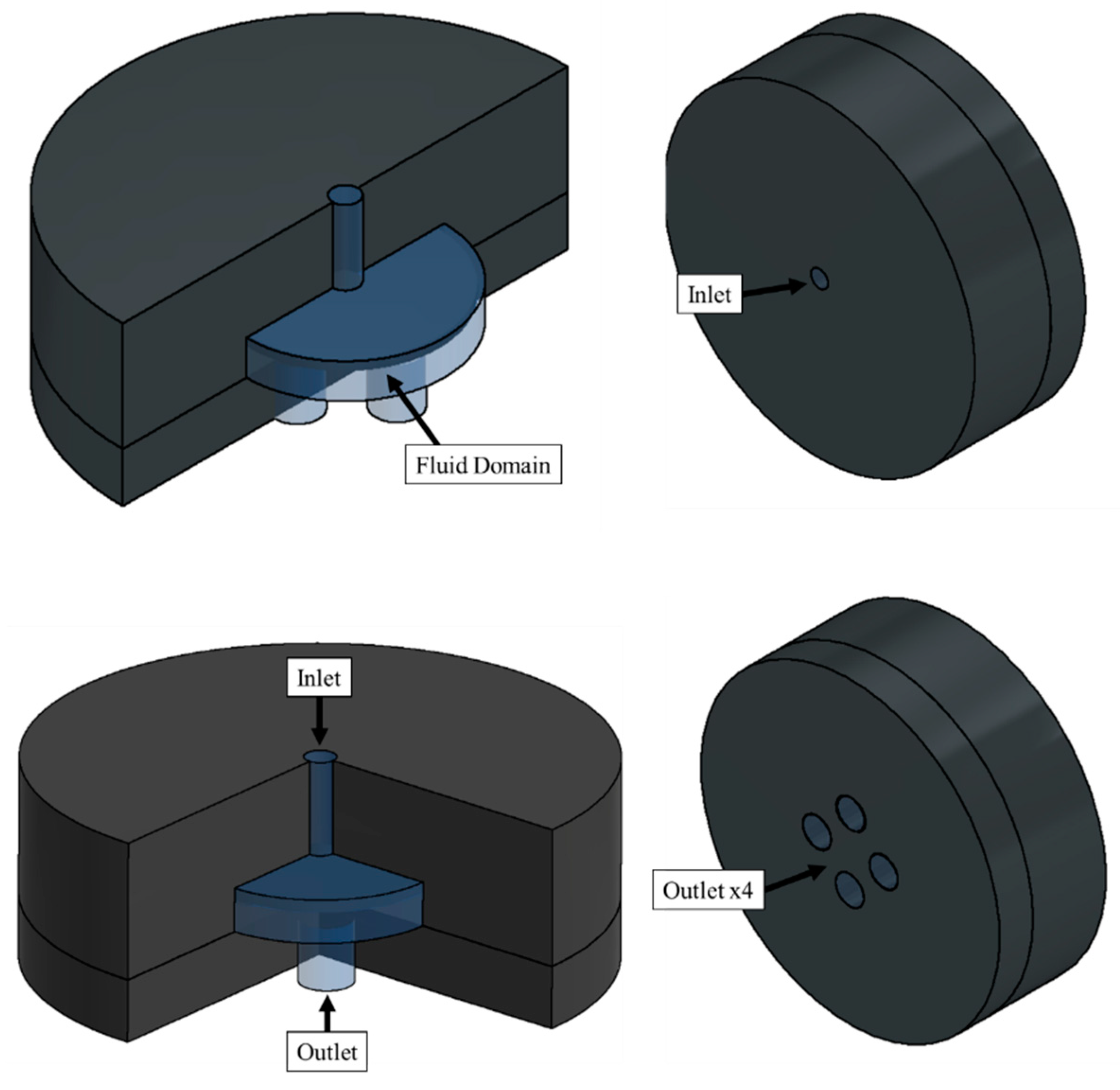
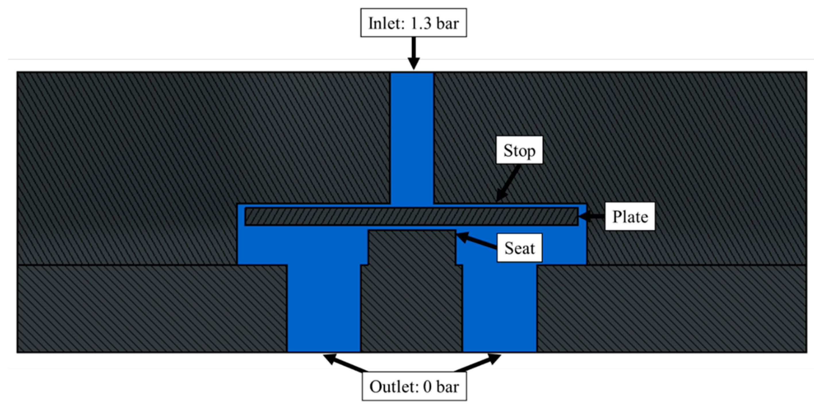
2.2.2. Domain, Initial, and Boundary Conditions for Validation
2.3. Discretization of the Domain
2.3.1. Mesh Independence through GCI Analysis
2.4. Turbulence Analysis
3. Results
3.1. Validation and Real-Case Analysis
3.1.1. Validation
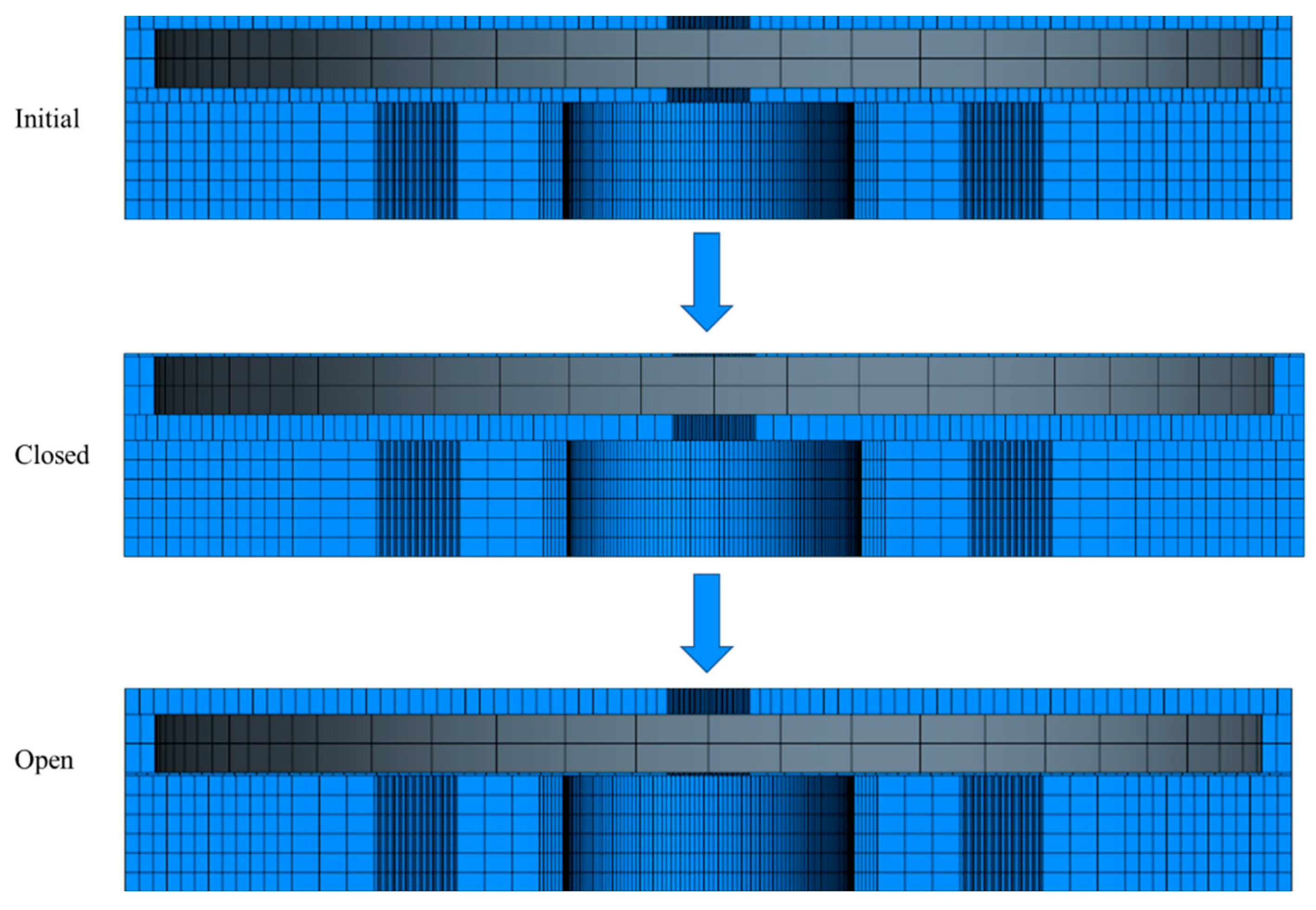
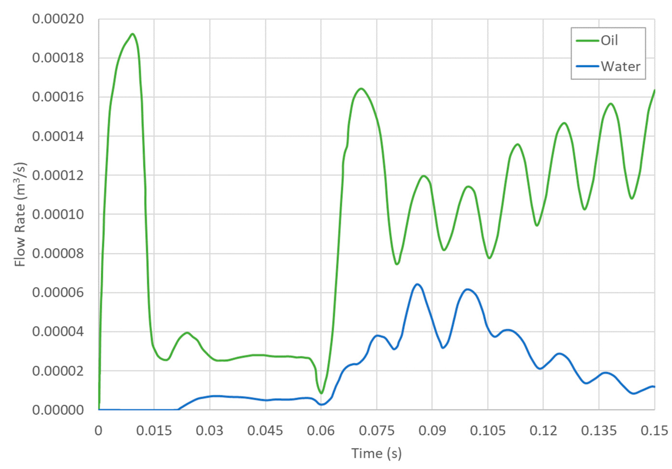
3.1.2. Multiphase Flow
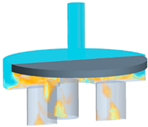
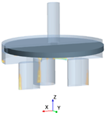
- The first stage (0.00 s): the domain was filled with oil, water began to flow in, and the plate was static in the middle of the chamber.
- The second stage (0.04 s): there was a quasistatic behavior in the plate’s motion in the closed position due to the water. In this step, the oil entered the valve again.
- The third stage (0.15 s): the water left the domain at the end of the process.
3.2. Mesh Independency
3.3. Turbulence Analysis
4. Conclusions
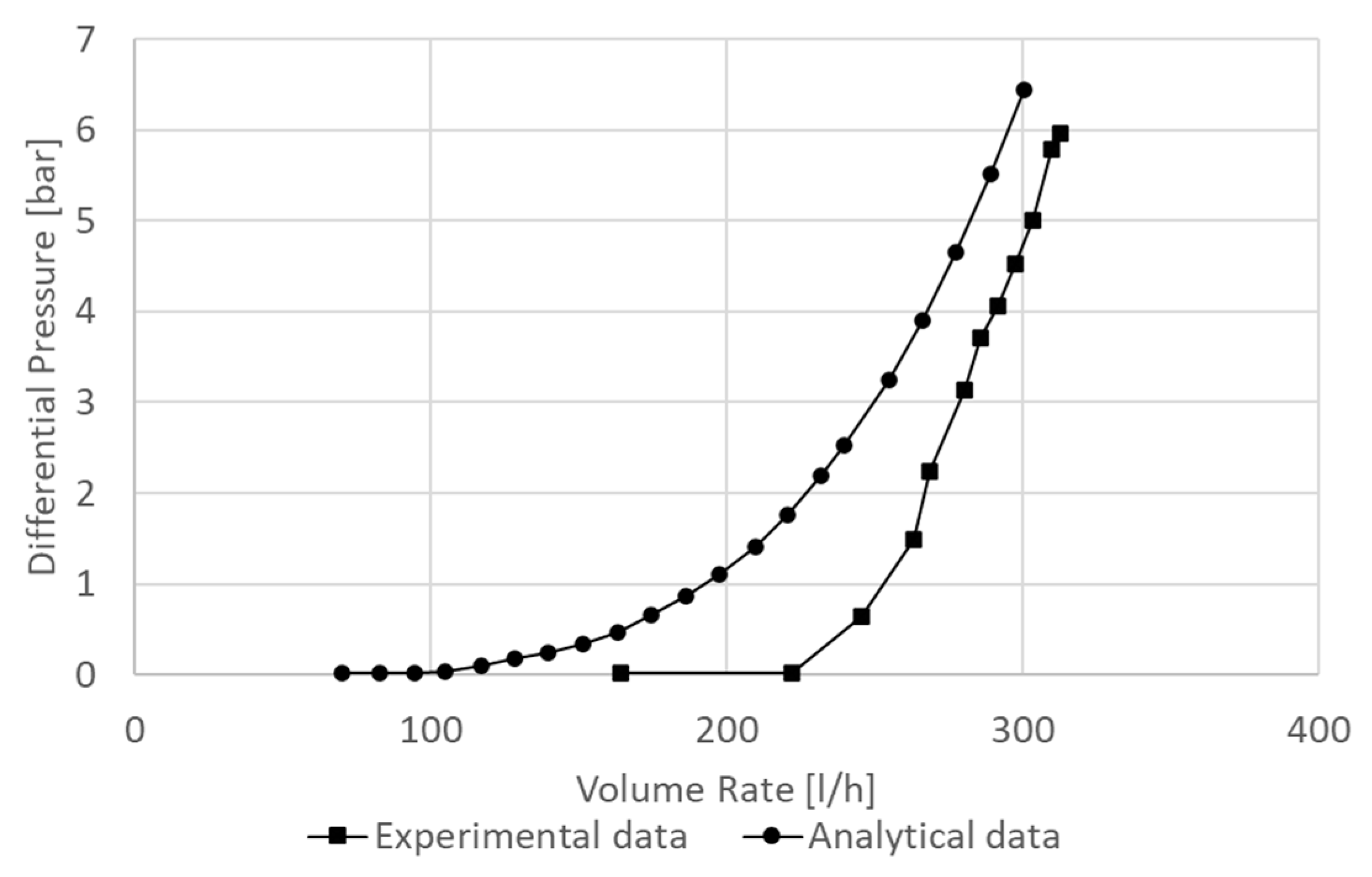
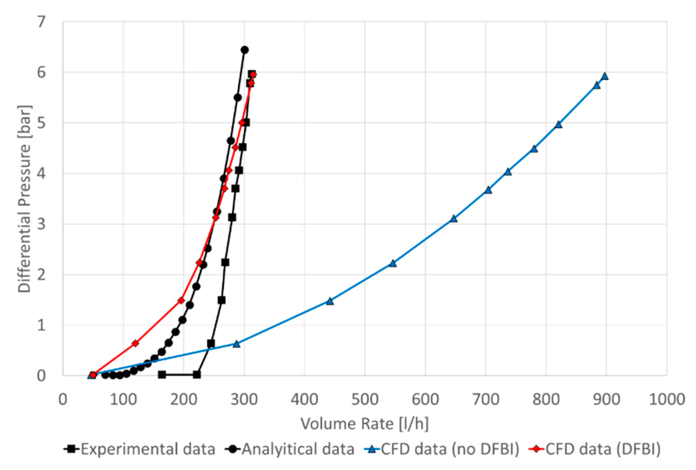
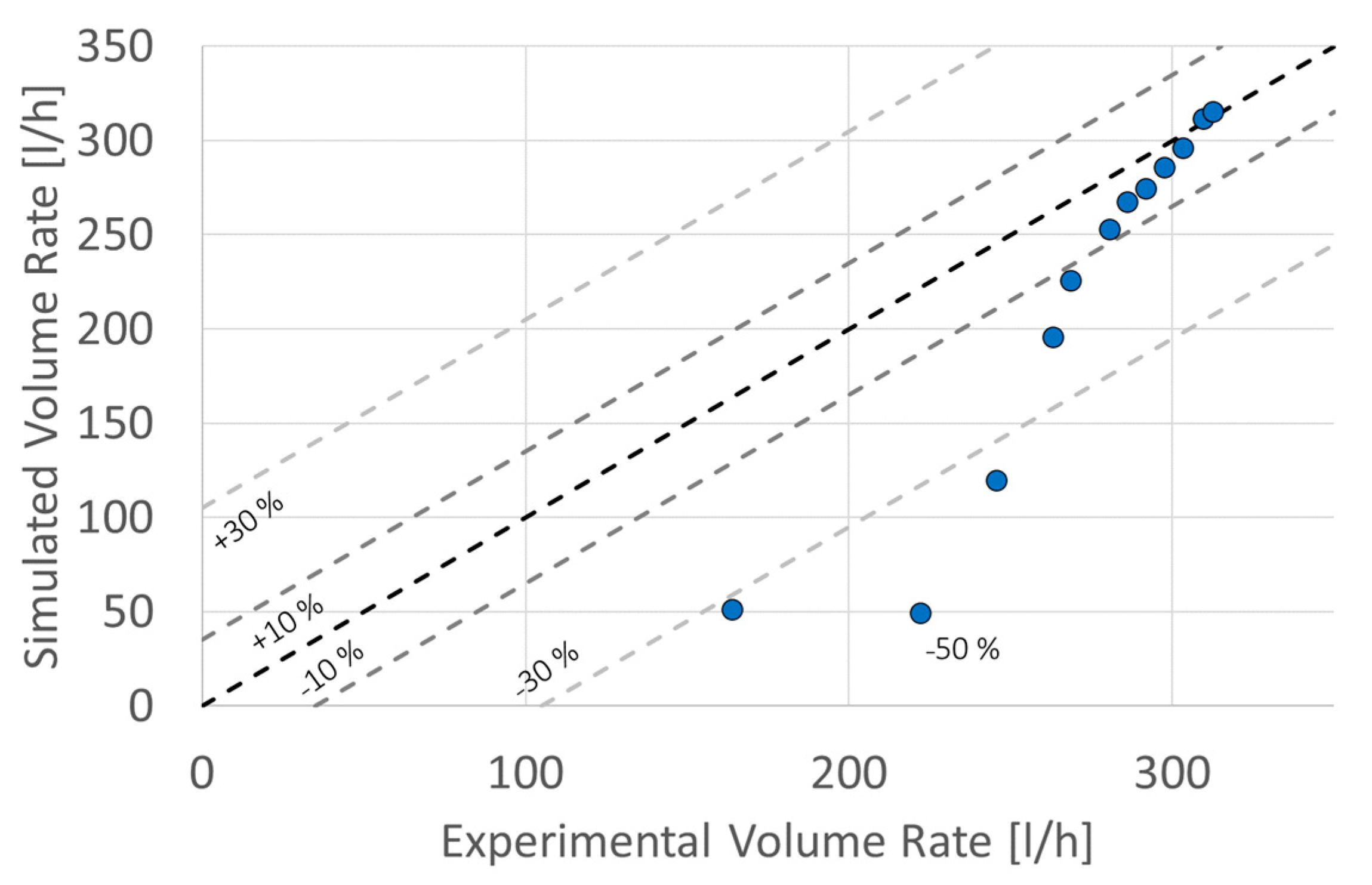
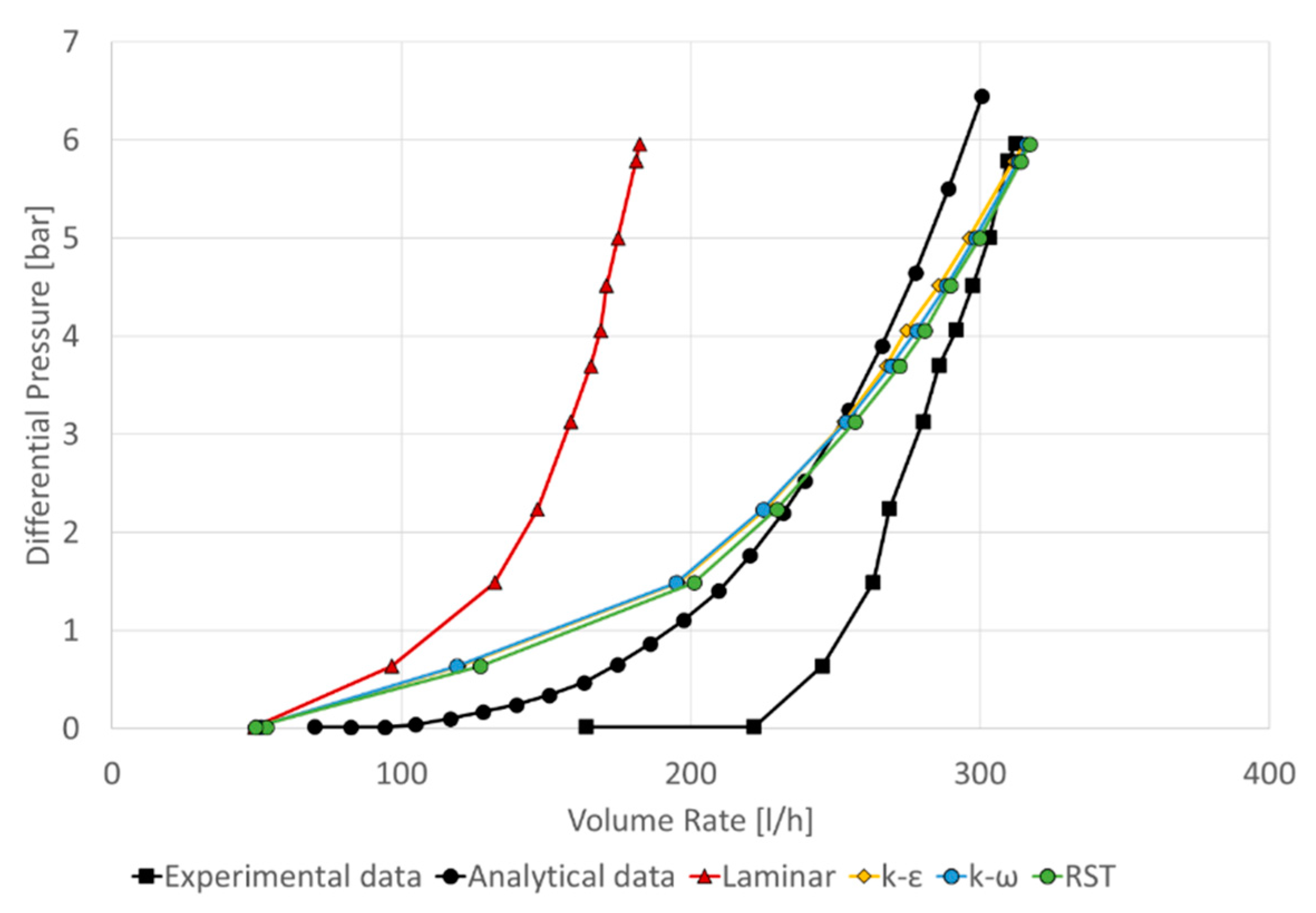
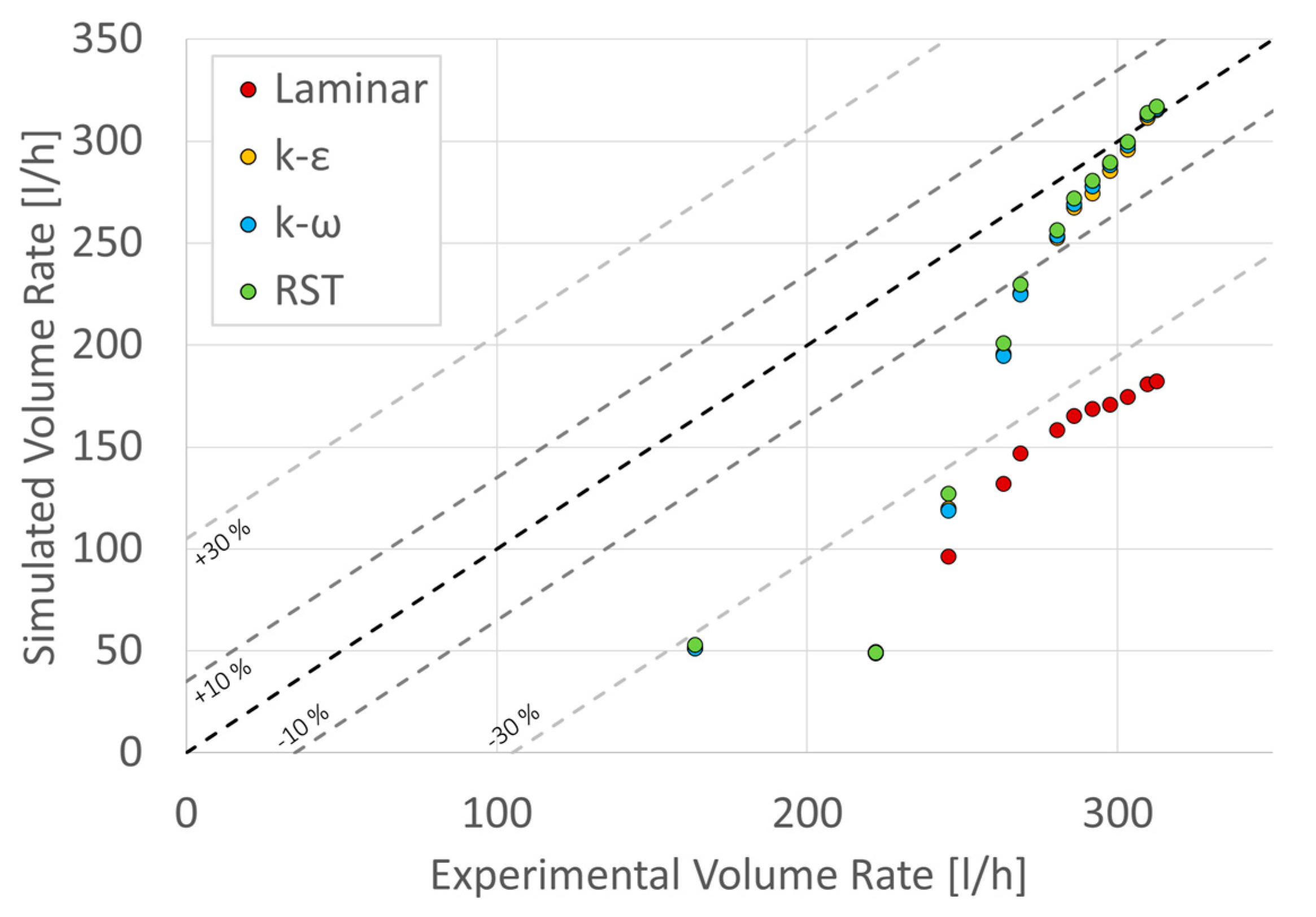
- The single-phase model using DFBI and mesh morphing showed excellent results in describing the valve behavior when choking occurred. This meant that the model prediction had a deviation between 30% and 50% for low-pressure differences compared to the experimental data. One reason for the deviation could be that the experimental data contemplated the flow dynamics upstream of the measurement point, which was not considered in the simulations. On the other hand, for high differential pressures, the error between experimental and simulated data was less than 10% when choking occurred. These pressure conditions were the most common in reservoirs reaching differential pressures up to 20 bar; however, Askvik and Johannessen could only reach up to 6 bar experimentally.
- In contrast, the model for low differential pressures fit the analytical data better, resulting in errors below 10%; this may have shown that conditions that were not considered in the analytical model and in the CFD model that was considered in the experimental process became evident for low pressures. Conditions such as material roughness, radial movements, and fluid emulsions, among others, could affect the solution. Therefore, the CFD model should consider that low differential pressure means low flow velocities close to regimes in transition; this implies that the turbulence models chosen should contemplate a correction for low Re. This condition is highly linked to having a y+ below 1, something that was not considered when designing the mesh.
- The prediction performed without the model plate’s motion resulted in values distant from the experimental data. This was expected because without body motion, the model did not analyze the natural behavior of an RCP.
- It was determined that mesh morphing and DFBI actively responded depending on the fluid flowing into the device when analyzing a real-life case. When water flowed in, the plate rose to plug the nozzle; the plate lowered and allowed the flow to pass through when oil flowed in.
- An essential consideration of the DFBI model was the need to add contact constraints on the inner walls of the valve to contain the plate properly. However, due to the geometric scale and the high velocities of the plate, setting the contact conditions was of high complexity. Therefore, one of the assumptions that had to be made for the model was to dampen the motion of the plate. This is evident in Figure 15, which shows that the plate’s translation oscillated when the water entered but was damped and remained constant until the oil enters. This did not occur in real life; the expected behavior was the plate closing when the inlet began to vibrate due to the pressure variations.
- Although there were difficulties in emulating the oscillation of the plate, the results obtained showed an excellent prediction of the valve’s performance, as shown in the validation of the model. Therefore, the present computational analysis and the model generated are recommended for predicting results such as the curves of the pressure difference versus the flow rate and analyzing the device’s behavior for different geometrical considerations to optimize the process.
- Mesh independence showed that the unsteady-state case had a lower GCI than the steady-state case. There was not much in the literature on applying this analysis method to models with mesh morphing.
- Assuming a laminar flow showed results far from reality (more than a 30% error). Few differences between models were found when a turbulent flow regime was considered. The RST model was the most complete among the RANS models because it described the domain’s flow dynamics, making it an excellent choice. However, the computational cost of this model was higher by 22% compared to the computational time for solving the two-equation models. Since the difference between the turbulent regime solutions was small, we recommend using the realizable k-ε or SST k-ω model.
- For future work, we recommend finding a method for implementing the contacts inside the valve so that the oscillations of the plate are replicated. Using the present model, it is possible to analyze conditions that Askvik and Johannessen could not detail in their experimental process due to operational problems such as reaching pressure conditions of 20 bar or analyzing different oil viscosities for the valve they designed. Something that can also be analyzed is the effect of the oil and gas flow inside the valve. Due to the density difference between the phases, it is expected that something similar will happen with the water at the gas inlet (the plate moving to a closed position).
- Sources of errors that could affect the validation of the model include a lack of information on the upstream and downstream data of the valve during the experimental process; these variations can affect the flow dynamics and cause the computational model to be far from reality. Another aspect of the experimental data was that it did not detail whether the valve was vertical or horizontal, which would change how gravity affected it; in this study, it was assumed that the valve was vertical. A final source of error was that only the motion of the plate in the vertical direction was considered and not in other possible directions, which may have affected the results in predicting the outflow. Finally, the mesh treatment for the no-slip condition was not considered, so parameters such as y+ were not analyzed; this could have caused the values obtained to be different from reality.
Author Contributions
Funding
Conflicts of Interest
Nomenclature
| Surface area (m2) | User-defined source term (-) | ||
| AICD | Autonomous inflow control device | Time (s) | |
| DFBI | Dynamic fluid–body interaction | Velocity of the fluid (m/s) | |
| Relative error (-) | Diffusion velocity (m2/s) | ||
| Extrapolated relative error (-) | Volume of i-phase in a cell (m3) | ||
| Gravity (m/s2) | Total volume of a cell (m3) | ||
| GCI | Grid convergence index | VOF | Volume of fluid |
| ICD | Inflow control device | Volume fraction of i-phase in a cell (-) | |
| ICV | Inflow control valve | Greek | |
| Mesh element count (-) | Solution at defined discretization (-) | ||
| Order of accuracy (-) | Extrapolated solution (-) | ||
| Pressure (Pa) | Viscosity (Pa·s) | ||
| PICD | Passive inflow control device | Viscosity of i-phase (Pa·s) | |
| Refinement ratio (-) | Density (kg/m3) | ||
| RCP | Rate controlled production | Density of i-phase (kg/m3) | |
| User-defined source term of i-phase (-) |
References
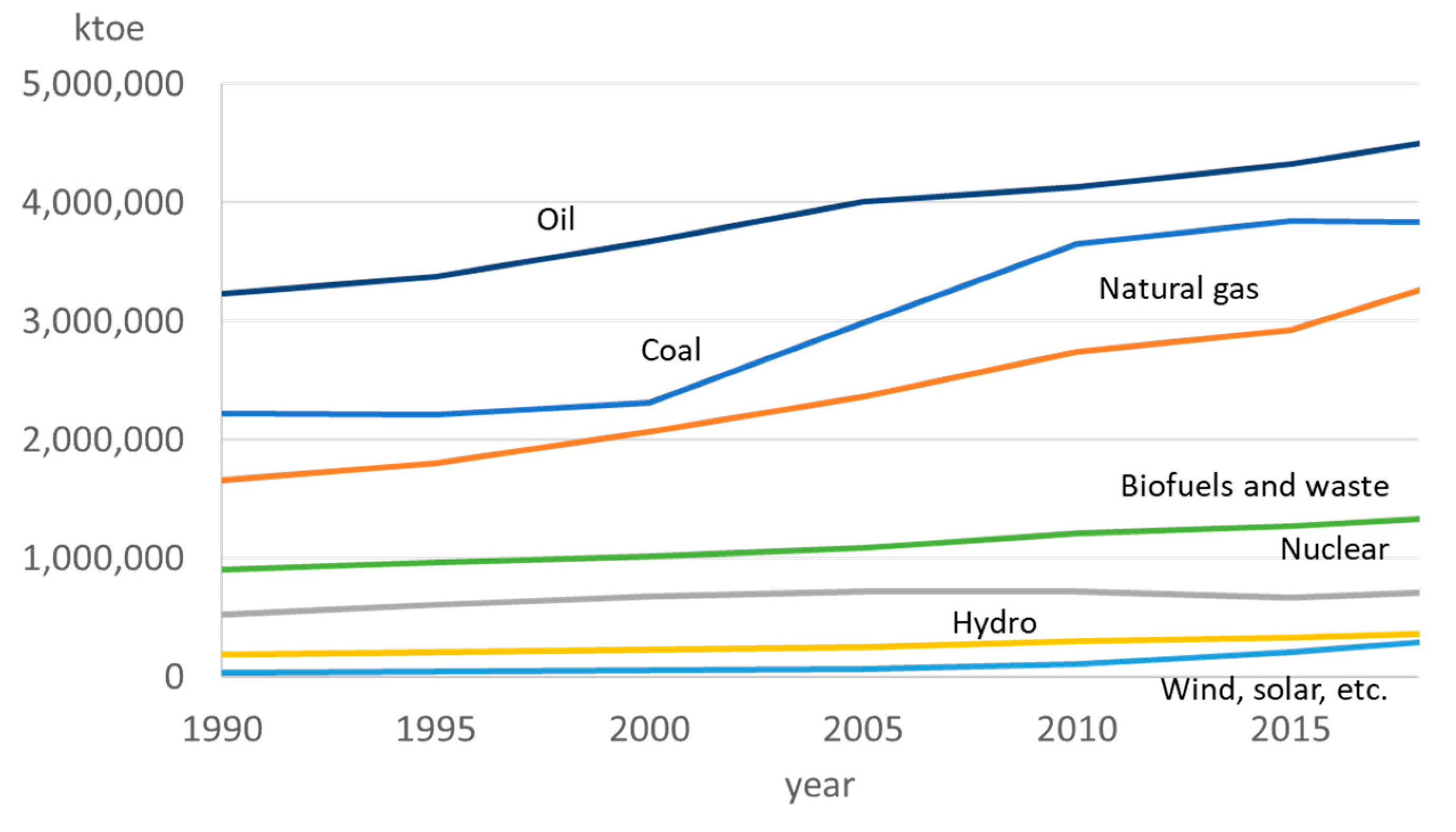
- IEA. Key World Energy Statistics 2020. IEA Publications. 2020. Available online: https://www.iea.org/reports/key-world-energy-statistics-2020 (accessed on 1 March 2021).
- Agencia Nacional Hidrocarburos. Colombia Open for Business. 2013. Available online: https://hydrocarbonscolombia.com/article/colombia-open-for-business/ (accessed on 1 March 2021).
- Bellaraby, J. Well Completion Design; Elsevier: Amsterdam, The Netherlands, 2009; Volume 56. [Google Scholar]
- Askvik, S.M.; Johannessen, I.L. Dynamic Autonomous Inflow Control Device; Norwegian University of Science and Technology: Trondheim, Norway, 2017. [Google Scholar]
- Halliburton. Inflow Control Devices. 2019. Available online: https://www.halliburton.com/en-US/ps/completions/sand-control/screens/inflow-control/default.html# (accessed on 23 May 2022).
- Zeng, Q.; Wang, Z.; Wang, X.; Li, Y.; Zou, W.; Xiao, J.; Chen, T.; Yang, G.; Zhang, Q. A novel autonomous inflow control device design: Improvements to hybrid ICD. In Proceedings of the International Petroleum Technology Conference 2014, IPTC 2014—Innovation and Collaboration: Keys to Affordable Energy, Kuala Lumpur, Malaysia, 10–12 December 2014; Volume 1, pp. 702–710. [Google Scholar]
- Fripp, M.; Zhao, L.; Least, B. The theory of a fluidic diode autonomous inflow control device. In Proceedings of the SPE Middle East Intelligent Energy Conference and Exhibition 2013, Manama, Bahrain, 28–30 October 2013; pp. 28–30. [Google Scholar]
- Corona, G.; Yin, W.; Felten, F. Enhanced nozzle inflow control device development for wall shear stress minimization in high-production application. In Proceedings of the Offshore Technology Conference, Houston, TX, USA, 2–5 May 2016; Volume 1, pp. 713–719. [Google Scholar]
- Versteeg, H.K.; Malalasekera, W. Chapter two: Conservation laws of fluid motion and boundary conditions. In An Introduction to Computational Fluid Dynamics: The Finite Volume Method; Pearson: Upper Saddle River, NJ, USA, 2007; pp. 9–39. [Google Scholar]
- Hirt, C.; Nichols, B. Volume of Fluid (VOF) method for the dynamics of free boundaries. J. Comput. Phys. 1981, 39, 201–225. [Google Scholar] [CrossRef]
- Versteeg, H.K.; Malalasekera, W. Chapter three: Turbulence and its modeling. In An Introduction to Computational Fluid Dynamics: The Finite Volume Method; Pearson: Upper Saddle River, NJ, USA, 2007; pp. 40–114. [Google Scholar]
- SIEMENS. 6-DOF Rigid Body Motion. Forces and Moments; SIEMENS: Munich, Germany, 2020; pp. 1–3. [Google Scholar]
- SIEMENS. 6-DOF Rigid Body Motion. Body Connections; SIEMENS: Munich, Germany, 2020; pp. 4–6. [Google Scholar]
- Argyropoulos, C.D.; Markatos, N.C. Recent advances on the numerical modelling of turbulent flows. Appl. Math. Model. 2015, 39, 693–732. [Google Scholar] [CrossRef]
- Celik, I.B.; Ghia, U.; Roache, P.J.; Freitas, C.J. Procedure for Estimation and Reporting of Uncertainty Due to Discretization in CFD Applications. J. Fluids Eng. 2008, 130, 078001. [Google Scholar]
- SIEMENS. Reynolds-Averaged Navier-Stokes (RANS) Turbulence Models; SIEMENS: Munich, Germany, 2021; pp. 1–3. [Google Scholar]


| Author and Year | Computational Model | ICD Modeled | Study Purpose |
|---|---|---|---|
| Fripp et al. (2013). [7] | CFD simulation | Fluidic diode | The second-generation technology of ICDs, the fluidic diode AICD, was analyzed for the first time; the production of the densest fluid (water) decreased because the device makes the entrance to the tubing more tortuous. The authors conducted single-phase CFD simulations in which the fluid properties changed. The study found that the AICD caused a vortex for water, thus delaying its production; while for oil, the path became less tortuous and the oil entered faster. |
| Corona et al. (2016). [8] | CFD simulation | PICD | Minimized the wall shear stress of an ICD, performed stationary single-phase CFD simulations, and analyzed the water flow’s turbulence when entering the device. The authors designed a device variation that minimized the shear stress and improved water production control. |
| Askvik and Johannessen (2017). [4] | CFD simulation | RCP | The authors changed the proposed Halvorsen RCP design and performed single-phase simulations in CFD to determine the new device’s internal flow patterns. However, the study focused on presenting an experimental design and contrasting it with analytical data; likewise, the authors constructed several curves by changing between geometric variables of the valve to determine their effect on the pressure difference and the flow rate. |
| Property | Value |
|---|---|
| Water viscosity (Pa s) | 0.001 |
| Oil viscosity (Pa s) | 0.064 |
| Water density (kg/m3) | 1000 |
| Oil density (kg/m3) | 857 |
| Interfacial tension (N/m) | 0.036 |
| Time (s) | Total Render | Chamber Render | Volume Fraction |
|---|---|---|---|
 |  |  | |
 |  |  | |
 |  |  | |
 | |||
| Parameter | Steady | Unsteady * | |
|---|---|---|---|
| 84,864 | |||
| 43,728 | |||
| 27,816 | |||
| 1.0864 | |||
| 1.1169 | |||
| Pressure Drop (bar) | 3.621 | 3.607 | |
| 3.597 | 3.698 | ||
| 3.586 | 3.349 | ||
| 5.030 | 23.229 | ||
| 3.667 | 3.591 | ||
| 0.007 | 0.025 | ||
| 0.013 | 0.004 | ||
| 0.016 | 0.005 | ||
| Flow rate (l/h) | 0.160 | 0.071 | |
| 0.175 | 0.074 | ||
| 0.172 | 0.159 | ||
| 15.275 | 60.690 | ||
| 0.154 | 0.071 | ||
| 0.094 | 0.042 | ||
| 0.038 | 2.786 × 10⁻⁴ | ||
| 0.046 | 3.481 × 10⁻⁴ | ||
| Mesh | N | Base Size Approach (mm) | Computational Time (h) |
|---|---|---|---|
| 1 | 84,864 | 0.764 | 12.739 |
| 2 | 43,728 | 0.830 | 11.644 |
| 3 | 27,816 | 0.927 | 10.642 |
Publisher’s Note: MDPI stays neutral with regard to jurisdictional claims in published maps and institutional affiliations. |
© 2022 by the authors. Licensee MDPI, Basel, Switzerland. This article is an open access article distributed under the terms and conditions of the Creative Commons Attribution (CC BY) license (https://creativecommons.org/licenses/by/4.0/).
Share and Cite
Cerquera, L.A.R.; Pinilla, J.A.; Ratkovich, N.R.; Asuaje, M. Study of the Dynamic Behavior of an Autonomous Inflow-Control Device Using a Digital Twin. Processes 2022, 10, 2691. https://doi.org/10.3390/pr10122691
Cerquera LAR, Pinilla JA, Ratkovich NR, Asuaje M. Study of the Dynamic Behavior of an Autonomous Inflow-Control Device Using a Digital Twin. Processes. 2022; 10(12):2691. https://doi.org/10.3390/pr10122691
Chicago/Turabian StyleCerquera, Luis Alfonso Ramirez, Jorge Andrés Pinilla, Nicolás Ríos Ratkovich, and Miguel Asuaje. 2022. "Study of the Dynamic Behavior of an Autonomous Inflow-Control Device Using a Digital Twin" Processes 10, no. 12: 2691. https://doi.org/10.3390/pr10122691
APA StyleCerquera, L. A. R., Pinilla, J. A., Ratkovich, N. R., & Asuaje, M. (2022). Study of the Dynamic Behavior of an Autonomous Inflow-Control Device Using a Digital Twin. Processes, 10(12), 2691. https://doi.org/10.3390/pr10122691