Article

Study on the Flow Pattern and Transition Criterion of Gas-Liquid Two-Phase Flow in the Annular of Shale Gas Fractured Horizontal Wells

1
Gas-Lift Technology Center of Tuha—CNPC, Shanshan, Turpan 838200, China
2
College of Petroleum Engineering, Yangtze University, Wuhan 430100, China
*
Author to whom correspondence should be addressed.
Processes 2022, 10(12), 2630; https://doi.org/10.3390/pr10122630
Submission received: 24 October 2022 / Revised: 15 November 2022 / Accepted: 1 December 2022 / Published: 7 December 2022

Abstract

:
Improving the accuracy of pressure prediction in the wellbore annular is of great importance for the design in oil and gas production. However, due to the existence of double-layer liquid membrane and the lack of relevant experiments, the existing correlations fail to the field application. In this study, a new model of flow pattern transition in inclined annulus pipe is proposed by using a mechanistic approach to classify the flow patterns. Firstly, a gas-liquid two-phase flow experiment in annulus pipe was carried out in a pipe with an outer diameter of 73.02 mm and an inner diameter of 121.36 mm, and then the influence of inclined angle on the transition boundary of flow pattern is discussed. Finally, a hydrodynamic transition criterion for the flow pattern model of inclined annulus pipe is established and verified in detail. The experimental results show that bubble flow, slug flow, churn flow and annular flow were observed under different inclination angles, and the results indicate that the slug flow will be shifted to the larger gas-liquid superficial flow rate region with the smaller inclination angle, and the annular flow will appear in the higher gas superficial flow rate region. Compared to the performance of the existing correlations (Kelessidis and Zhang) and the present model using the experimental data, the accuracy of the new model reached 83%, significantly higher than the other two models, and the new correlation was better in predicting the transition from slug flow to churn flow and churn flow to annular flow.

1. Introduction

Hydraulic fracturing can effectively improve the recovery rate of shale gas and has become the main development method of shale gas fields. However, the flowback of shale gas fracturing fluid is complex and easy to accumulate fluid, which seriously restricts gas well productivity [1,2]. Prediction of pressure drop in annulus pipe is the basis for determining shale gas wellbore fluid accumulation and drainage process preferences. In addition, the conventional oil and gas extraction process, such as underbalanced drilling and spontaneous injection wells at high production rates, will involve the flow of two-phase flow in annulus pipe [3].
The division of flow pattern boundaries is a prerequisite for the calculation of annular air-water two-phase flow parameters. However, the flow patterns, especially slug flow and annular flow, in the annulus pipe are different from those in the circular pipe. There are two liquid films in the annular two-phase flow, one is the casing film in contact with the casing wall (or well wall), and the other is the tubing film in contact with the tubing wall. In addition, according to the experimental observations of Caetano [4], Taylor bubbles are no longer symmetrical and there is a region of high turbulence behind the Taylor bubble, due to the presence of a channel connecting the tubular membrane to the casing membrane in the dorsal direction. The annular flow in the annulus pipe occurs at very high gas flow rates, the gas phase contains liquid droplets, and a very thin liquid film around the core. Due to the structure of the annular, two liquid films also exist, an inner film in contact with the tubing wall and an outer film in contact with the casing wall, the outer film being thicker than the inner film. At high superficial liquid-phase flow rates, Taitel [5] suggested that turbulent disturbance forces cause the gas phase in a bubbling or elastomeric flow to shatter into smaller bubbles, which are dispersed inside the continuous liquid phase. When the turbulence intensity can be sufficient to disperse Taylor bubbles into smaller bubbles than the critical bubble size, it will prevent them from re-aggregating, and the dispersed bubble flow will occur.
Few studies are devoted to its flow pattern and flow pattern distribution diagram. The accuracy of transition prediction for slug flow and annular flow is poor. There are even fewer studies on the flow pattern of inclined pipe annular two-phase flow. In 1982, Sadatomi studied two-phase flow in a non-circular pipe with air and water [6]. He studied the flow pattern and pressure drop of gas-liquid two-phase flow in a vertical concentric annulus pipe with a diameter ratio N of 0.5. However, he classified the types of flow patterns roughly and did not give a specific model for the transition between flow patterns. In 1989, Kelessidis measured the local gas content of in annulus pipe by the electric probe method and studied on the transition of flow patterns, in which the bubbly flow was predicted more accurately and the slug flow, and annular flow were predicted with larger errors [7]. In 1992, Caetano gave a more detailed description of the types of flow patterns and the characteristics different from those of circular pipe flow patterns [4]. Taitel’s circular pipe flow pattern transition model was modified and applied to vertical annulus pipe. The flow pattern distribution of vertical concentric and vertical eccentric annulus pipe was given. In 1992, Hasan applied the drift flow model to investigate the gas content rate of the annular flow pattern. A correction was presented to the calculation equation for the rise velocity of Taylor bubble, and a more accurate equation for the calculation of the gas content rate of inclined pipe annular was obtained [8]. In 2003, Zhang established a vertical annular hollow pipe section slug flow and annular flow transition model, and studied the vertical annular air-liquid two-phase flow with inner pipe rotation [9]. In 2014, Yin established a hydrodynamic model applicable to vertical and inclined tubular annular air-liquid two-phase flow, and modified the annular flow pattern transition criterion, which has better accuracy compared to the previous models [10].
At present, the studies for the annular air-liquid two-phase flow in wellbore are based on vertical and horizontal pipes [11,12,13,14,15,16,17,18,19,20,21]. Mostly, the concept of equivalent diameter is used to analyze and calculate with the help of the circular pipe method. There are fewer studies on the two-phase flow in the annular of inclined pipes. Due to the influence of pipe inclination on the flow pattern of annular two-phase flow, and the existence of a double liquid film, the flow state in the annulus pipe is more complex than the circular pipe flow. Therefore, the direct application of the vertical pipe flow pattern transition criterion may lead to large errors.
Due to the complex characteristics of annular air liquid two-phase flow and the lack of relevant experiments, in this study, a gas-liquid two-phase flow experiment in annulus pipe was carried out, and then the influence of inclined angle on the transition boundary of flow pattern is discussed. The experimental results indicate that the slug flow will be shifted to the larger gas-liquid superficial flow rate region with the smaller inclination angle, and the annular flow will appear in the higher gas superficial flow rate region. A hydrodynamic transition criterion for the flow pattern model of inclined annulus pipe is established and verified in detail, the results show that the new correlation has better performance in predicting the transition from slug flow to churn flow, and churn flow to annular flow.

2. Experiment and Analysis

2.1. Experimental Setup and Process

The experiments were conducted in the multiphase flow experimental platform of CNPC (China National Petroleum Corporation), as shown in Figure 1. The platform can carry out the study of multiphase pipe flow dynamics in single-phase, gas-liquid two-phase, and oil-gas-water three-phase under various conditions such as different inclination angles and different gas-liquid velocities. The platform is composed of nine parts, including simulated wellbore, oil-water stabilization system, gas stabilization system, and cooling water system. It is equipped with independent metering modules such as gas and liquid flow standard devices and piston type manometer standard devices, respectively. The accuracy of liquid flow meter is 0.3%, gas flow meter is 1%, and the accuracy of differential pressure sensor can be up to 0.25%, and high-speed camera frequency is 500 fps with a resolution of 1920 × 1080, which provides guarantee for the accuracy of measurement of experimental results.
The experiment was conducted in an annulus pipe with an outer diameter of 73.02 mm and an inner diameter of 121.36 mm. The experimental length of the pipe is 7.55 m, and the distance of the quick-closing valve is 11.32 m. The liquid-phase is water, and the gas-phase is air. In the room temperature of 11~14 °C environment, the specific experimental operations are as follows. The range of experimental parameters as shown in Table 1.

2.2. Analysis of Experimental Results

In the experiment, bubble flow, slug flow, churn flow, and annular flow can be observed, and the flow patterns were captured by high-speed camera. The experimental phenomena and results of different inclination angles are shown in Figure 2, Figure 3, Figure 4 and Figure 5.
In the experiment, the slug flow consists of the air embolism zone and the liquid embolism zone. The Taylor bubble and the liquid film around it can be observed in the segment plug flow gas bolus region. When the gas flow velocity (range from 0.4 m/s to 7.8 m/s) is small, the liquid film in the gas embolus area will show obvious liquid fall back due to the effect of gravity. The returned liquid flows along the underside of the annulus pipe to form a flow channel. When the gas flow velocity continues to increase (greater than 7.8 m/s), the liquid backflow phenomenon weakens, and the segment plug frequency accelerates and gradually transforms to churn flow. After the superficial gas flow velocity is greater than 15 m/s, it can be observed that the flow pattern gradually transforms to annular flow. The gas is in the middle of the annular space, and the liquid adhere to the annulus pipe wall to form a double-layer liquid film.
When the physical parameters of medium, pipe diameter, gas and liquid superficial flow velocities are determined, the flow patterns of Kelessidis [7], Caetano [4], Hasan [8], and Zhang [9] can be plotted, as shown in Figure 6. From the figure, it can be found that all the above four flow pattern prediction models can accurately predict the transition boundary between the bubbly flow and the slug flow. However, there are large errors in the transition from slug flow to churn flow, and churn flow to annular flow. Among them, the transition boundaries predicted by Hasan [8] and Caetano [4] models differ greatly from the experimental data. The experimental data show that the superficial gas velocity increases with the increase in the superficial liquid velocity during the transition from the churn flow to the annular flow. The superficial gas velocity is not constant as predicted by the Hasan [8] and Caetano [4] model. Compared to the Kelessidis [7] model, the boundary trend of the transition from slug flow to churn flow is more accurately predicted by the Zhang [9] model, but the superficial gas velocity is shifted in a smaller direction. The Kelessidis [7] model is more consistent with the present experimental data in the boundary prediction of the transition from churn flow to slug flow.
The flow pattern observed in the experiment at different angles were plotted, as shown in Figure 7, Figure 8 and Figure 9. From the experiment, it can be observed that when the tilt angle is changed, the transition boundary from slug flow to churn flow and annular flow will be shifted significantly. When the tilt angle is changed from 90° to 30°, the transition boundary of the slug flow to the churn flow and the annular flow also shifts to the direction of greater superficial gas flow velocity. Since the Kelessidis [7] and Zhang [9] model only gives the flow transition boundary of the vertical annulus pipe, it cannot accurately predict the flow transition of the inclined pipe. Therefore, it can be seen that when the annulus pipe is inclined, the liquid film at the bottom becomes thicker due to the influence of gravity. The shapes of bubbles in complex flow patterns such as slug flow are changed. There is also a special double liquid film in the annulus pipe, the flow state in the annulus pipe is more complicated than the circular pipe flow. Therefore, the direct application of the vertical pipe flow pattern transition formula may lead to large errors.
In this paper, the flow pattern discriminant diagrams of Kelessidis [7] and Zhang [9] models will be modified by combining experimental phenomena. The flow pattern is classified by using the mechanism approach and a new flow transition model for the slug flow in the inclined annulus pipe section is proposed.

3. Model Building and Discussion

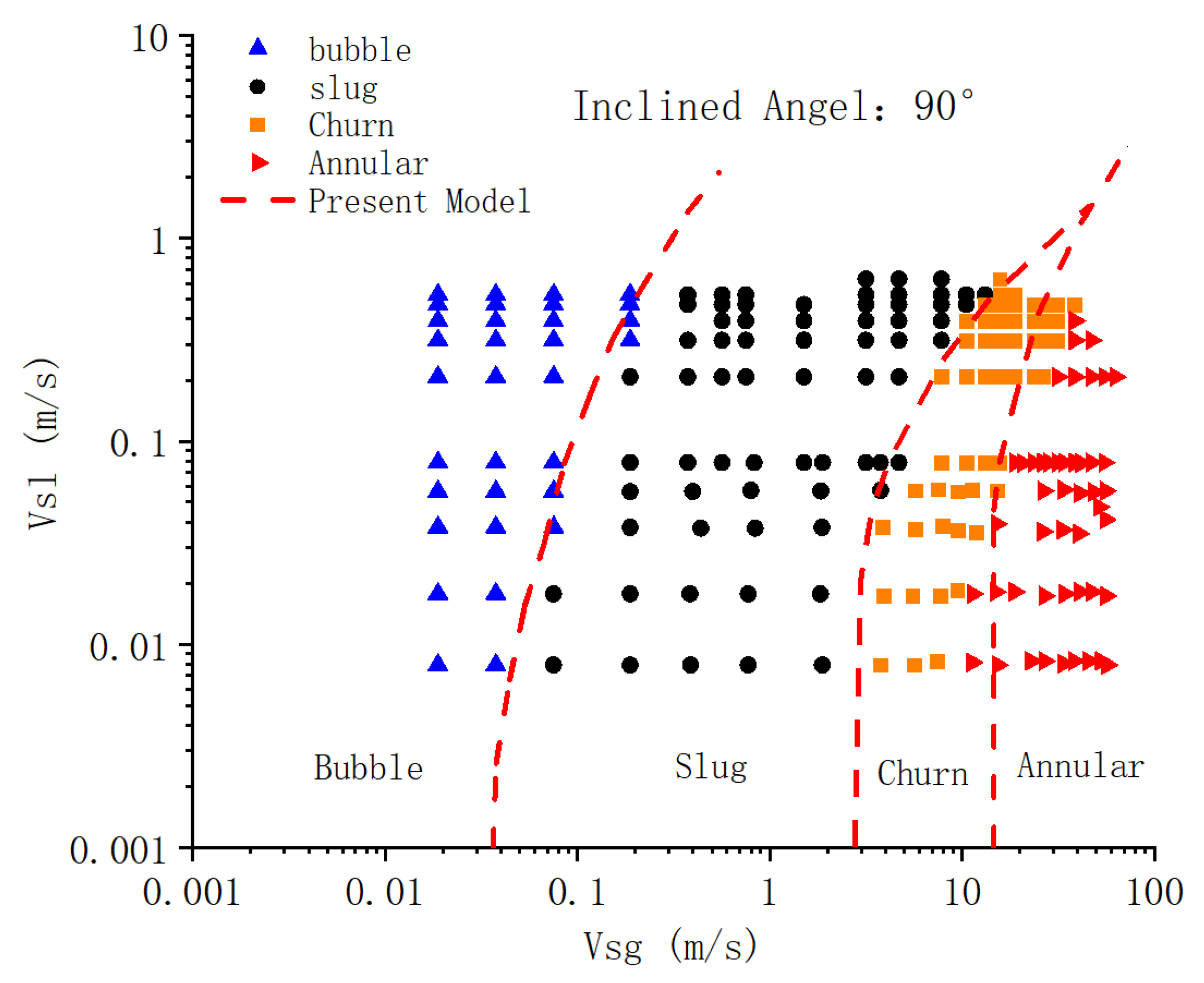
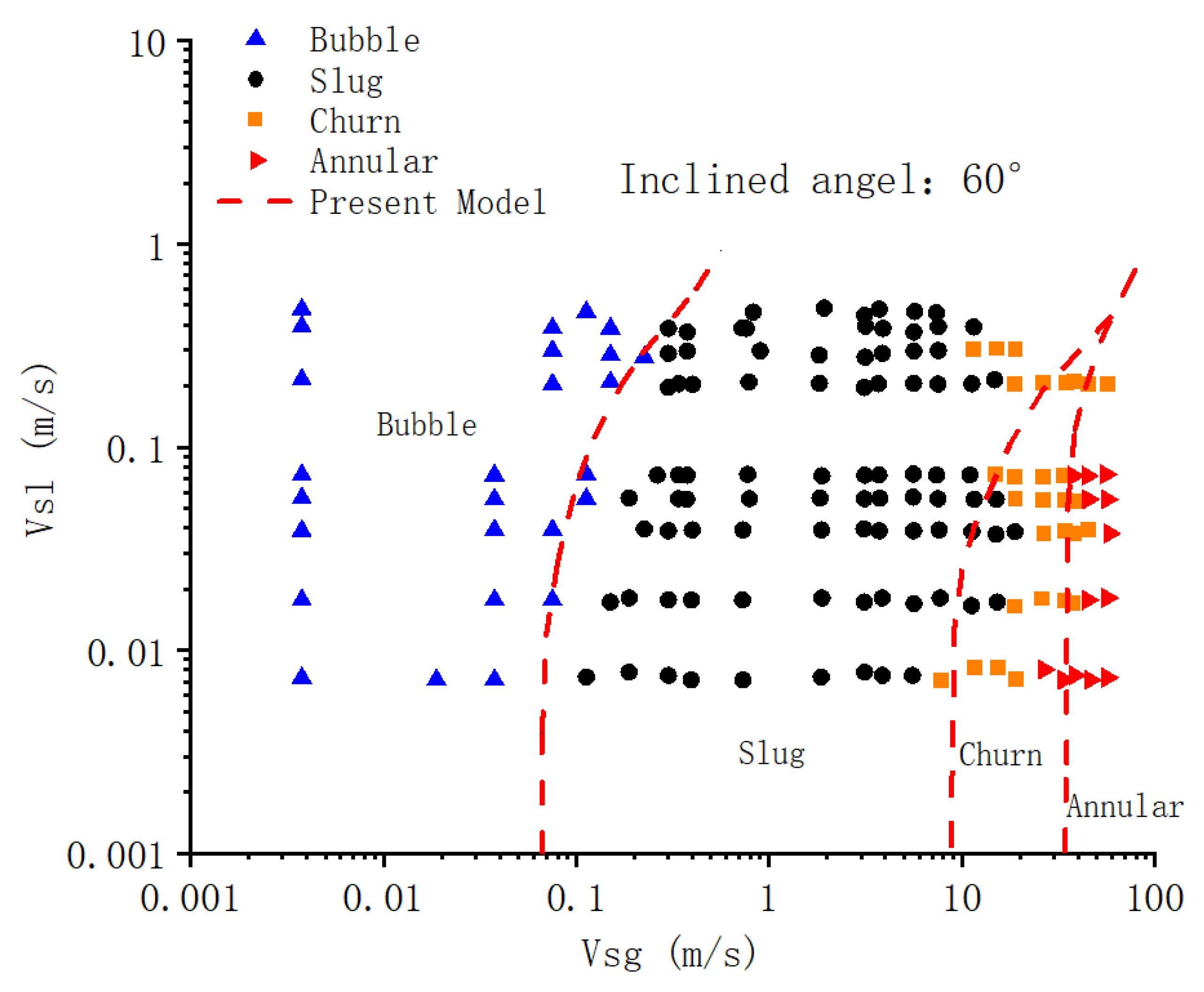
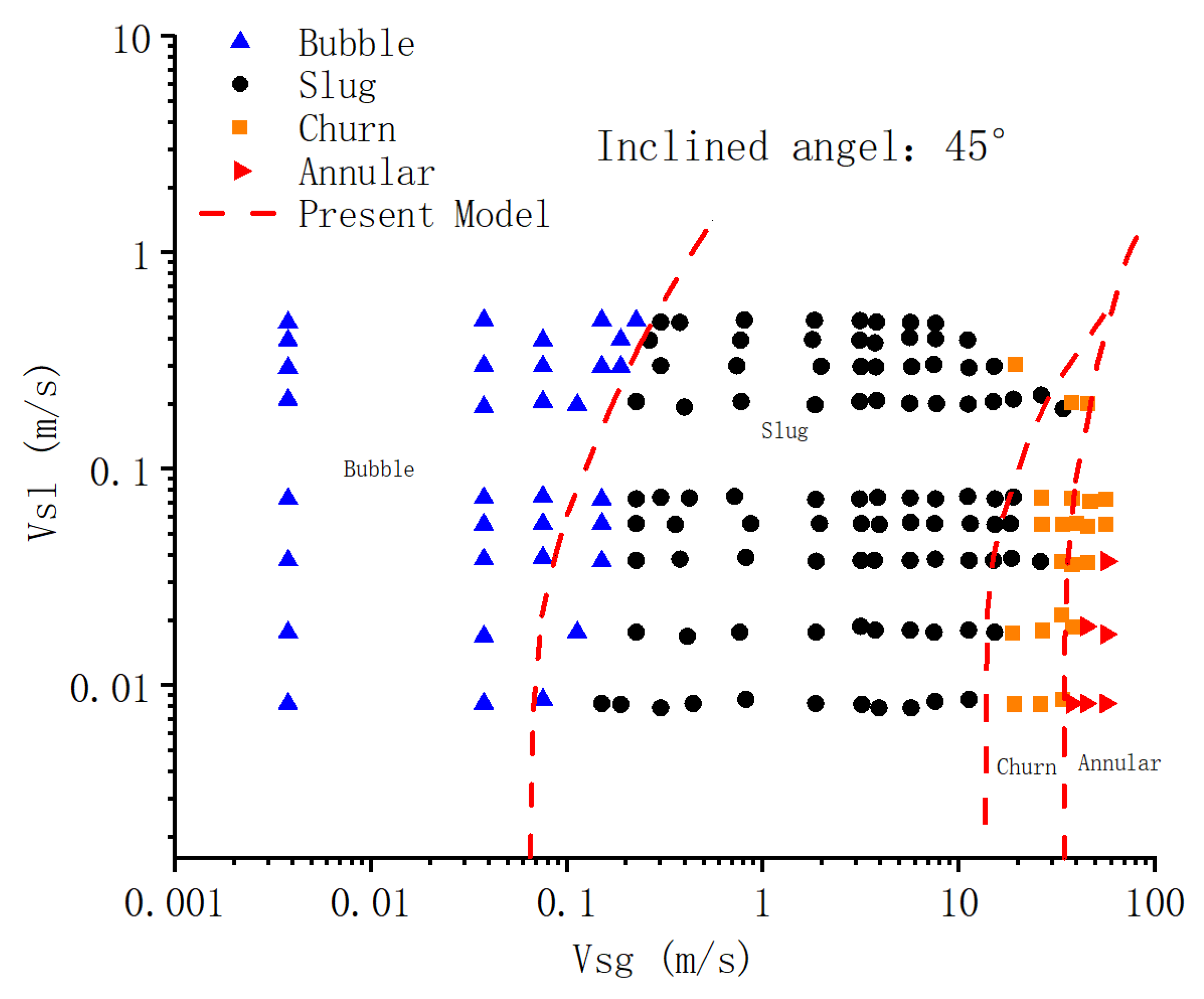
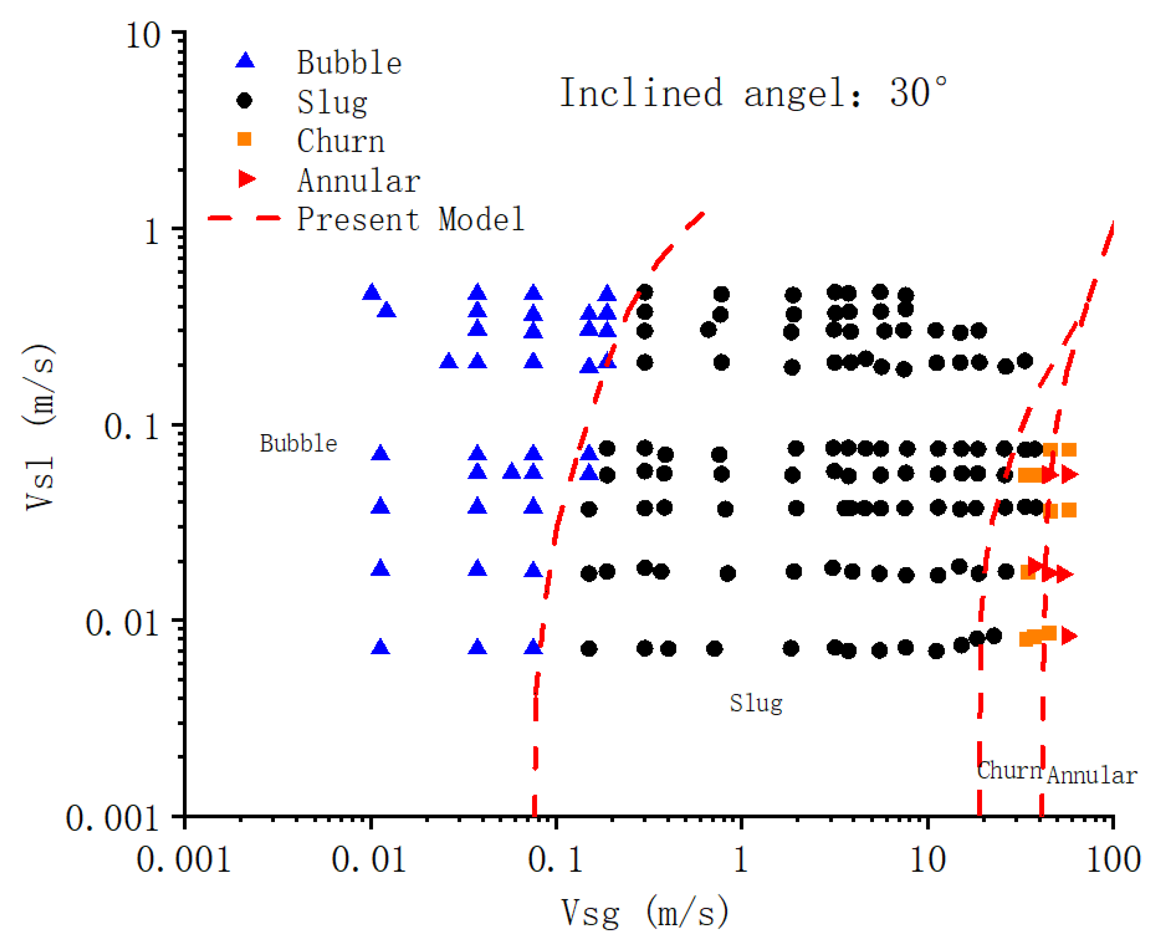
3.1. Establishment of the Flow Model for the Slug Flow in The Annulus Pipe Section

Most of the existing annular flow pattern transition guidelines are established in vertical pipe conditions. However, due to the influence of gravity, the gas-liquid distribution of the inclined pipe slug flow is very different compared to that of the vertical pipe. From the experimental observation, it is clear that the liquid phase of the slug flow in the inclined annulus pipe becomes asymmetrically distributed. In the middle of the double liquid film of the annulus pipe, a preferential channel is formed. This paper is based on the dynamic model of the slug flow in the annulus pipe. The effects of gas-liquid slip and negative frictional pressure drop are considered. The mass conservation and momentum conservation analysis is carried out for the annular slug unit body. 
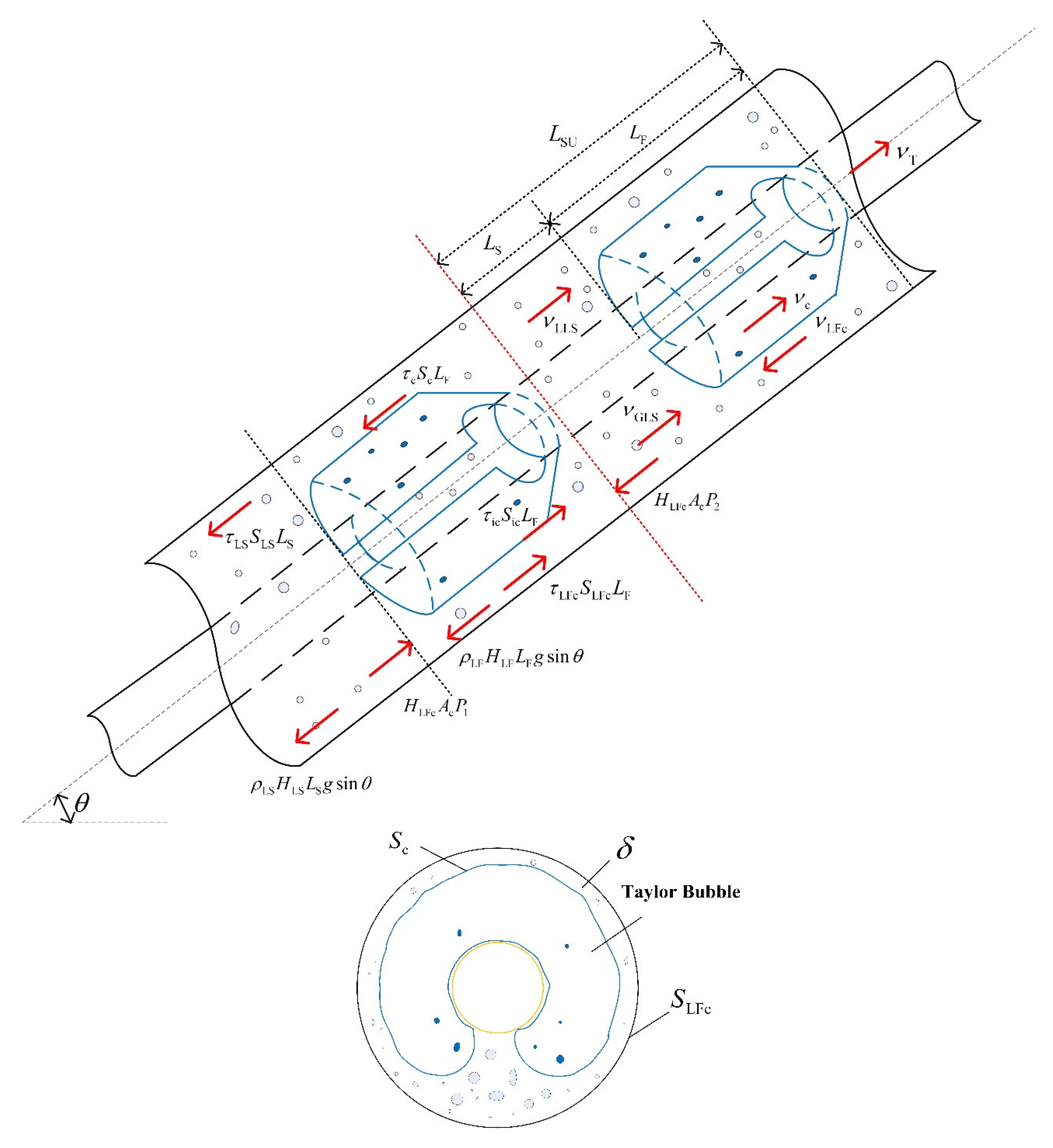
Figure 10 shows the schematic diagram of the velocity and force analysis of the slug flow in the annulus pipe.
The casing film is much thicker than the oil pipe film in the gas embolism area, the oil pipe film H LFd is much smaller than the casing film H LFc . The oil pipe membrane is much smaller than the casing membrane. Therefore, the oil pipe film is ignored in the slug flow model of this paper.
According to the experimental observation, the slug flow unit in steady state can be composed of a Taylor bubble and a section of liquid bolus. In the middle of the Taylor bubble, a preferential channel is formed. The fluid in the air bolus area will flow backward through this channel. It is assumed that the fluid in the control body of the cell is incompressible. The mass of the liquid phase flowing in from the bottom boundary of the liquid film is equal to the mass of the liquid phase flowing out from the top boundary of the liquid film.
v T v LLS H LS = v T + v LFc H LFc + v T v c H Lc
where: v T is the liquid slug transport velocity, m / s . v LLS is the liquid phase flow velocity in the liquid slug area, m / s . H LS is the liquid holding rate in the liquid slug area, %. v LFc is the casing membrane flow velocity, m / s . H LFc is the casing membrane holding rate, %. v c is the Taylor bubble flow velocity, and m / s . H Lc is the Taylor bubble holding rate, %.
Similarly, the mass of the gas phase entering the liquid membrane is equal to the mass of the gas phase leaving the liquid membrane. The mass conservation equation can be established.
( 1 H LS ) ( v T v GLS ) = ( v T v c ) ( 1 H LFc H Lc )
where, v GLS is the gas phase flow velocity in the liquid bolus region, m / s .
Consider the liquid and gas in the liquid bolus region there is a slippage situation, the gas flow rate v GLS should be greater than the liquid flow rate v LLS . Combined with the slip velocity defined by Caetano [4] in the following equation.
v s = v GLS v LLS = 1.53 ( ρ l ρ g ) g σ ρ l 2 0 . 25 ( H LS ) 0 . 5
v LLS = ( v sl + v sg ) 1.53 ( ρ l ρ g ) g σ ρ l 2 0 . 25 ( H LS ) 0 . 5 ( 1 H LS )
where, v s is the liquid slug flow rate, m / s . v sl is the liquid superficial flow rate, m / s . v sg is the gas superficial flow rate, m / s . ρ l is the liquid phase bulk density, and kg / m 3 . ρ g is the gas phase bulk density, kg / m 3 .
Therefore, combining the above equation yields.
v LFc H LFc = v s H LS + ( 1 H LFc ) v c v GLS
According to Zhang [9], the equation for the gas content in the liquid bolus region is known.
α s = v sg C 2 + C 3 v m
where, for the values of C 2 and C 3 , Schmidt [22] gave values of 0.331 and 1.25. Zhang [9] suggested that 0.425 and 2.65 are more applicable for the annular, and the liquid holding rate H LS in the liquid bolus region can be calculated.
H LS = 1 α s
Since the liquid content rate and the tubular membrane holding rate in Taylor bubble are much smaller than the casing membrane. Therefore, the casing membrane liquid-holding rate H LFc can be approximately equal to the liquid-holding rate H LF in the gas embolism zone.
H LF = 4 D C D C + D T δ D e 4 D e D C + D T δ D e 2
L LS L SU = v sl + v LFc H LF v LLS H LS + v LFc H LF
where, D C is the casing diameter, m. D T is the tubing diameter, m. D e is the annular hollow pipe hydraulic diameter, m. δ is the casing liquid film thickness, m. L LS is the liquid plug zone length, and m. L SU is the segment plug unit length, m.
From the cross-sectional diagram of the slug flow in Figure 10, it can be seen that Taylor bubble do not occupy the total cross-sectional area of the pipe. Instead, a preferential channel is formed. The liquid film around the Taylor bubble wets the tubing and casing wall through the priority channel. The liquid film thickness is calculated using the average casing liquid film converted thickness with the following equation.
δ = 9 . 06 × 10 9 3 υ l v TB 2 g D e / 2 δ 0.733
where, υ l is the liquid phase kinematic viscosity, Pa s . v TB is the Taylor bubble kinematic velocity, m / s .
According to the empirical equation of Zhang [9], the equation of the thickness of the falling liquid film around the Taylor bubble is shown in the following equation.
δ ( ρ l ρ g ) g ρ l υ l 2 1 / 3 = k Re f m
where, k and m are related to the flow pattern, and the values taken in this paper are k = 0.0682 and m = 2/3.
Re f = 4 v LFc δ υ l
From Equations (10)–(12), the liquid film flow velocity can be found. Combined with the mass conservation equation, the Taylor bubble flow velocity v c can be calculated.
The force analysis of the casing film and Taylor bubble in the air embolism area in the slug flow unit of the annular section is carried out separately, which is known according to the law of conservation of momentum.
H LF A c Δ P L LF = H LF A c ρ l g sin θ τ LFc S LFc τ ic S ic
( 1 H LF ) A c Δ P L LF = ( 1 H LF ) A c ρ g g sin θ + τ c S c + τ ic S ic
Similarly, the conservation of momentum within the liquid bolus.
H LS A c Δ P L LS = H LS A c ρ l g sin θ + τ LS S LS
where, τ LFc is the shear force at the contact interface between the casing wall and the casing membrane, Pa . τ c is the shear force at the contact interface between the casing liquid membrane and the Taylor bubble, Pa . τ LS is the shear force at the contact surface between the liquid slug and the casing membrane tubular membrane, Pa . S LFc is the wet perimeter of the casing wall, m. S c is the wet perimeter of the Taylor bubble, m. S ic is the wet perimeter of the contact interface between the casing membrane and the Taylor bubble, and m. S id is the wet perimeter of the contact interface between the tubular membrane and the Taylor bubble, m. According to Yin [10], the wall shear force in the flow conservation equation of the annular section slug is calculated as follows.
τ LFc = f LFc ρ LF v LFc 2 / 2
τ c = f c ρ c v c 2 / 2
τ LS S LS A c = 2 f s D e ρ s ( v sg + v sl ) 2
Friction factors:
f LFc = C 1 Re LFc a
f c = C 2 Re c b
f s = C 3 Re s c
where, f LFc is the friction factor of casing film. f c is the friction factor of tubing film. f s is the friction factor of Taylor bubble.
The hydrodynamic equivalent diameter method is used. The Reynolds number at the interface between the casing film, the tubing film, and the Taylor bubble can be expressed as the following equation.
Re LFc = v LFc ρ LF d LFc μ LF ,   d LFc = 4 H LF A c ( S LFc + S c )
Re c = v c ρ c d c μ c ,   d c = 4 ( 1 H LF ) A c S c
Re s = v LS ρ LS d LS μ LS ,   d LS = π ( D C + D T )
where, Re LFc is the Reynolds number of casing film. Re c is the Reynolds number of tubing film. Re s is the Reynolds number of Taylor bubble.
Wet Week:
S LFc = π D C
S c = S Ic + S Id = ( D C 2 δ + D T ) π + D e 2 δ

3.2. Inclined Annulus Pipe Flow Pattern Transition Criterion

Based on the formation mechanism of different flow patterns, this paper establishes the transition criterion of flow pattern in the annulus pipe on the basis of previous research results.

3.2.1. Transition from Bubble Flow to Slug Flow

The decisive role in the transition from bubble flow to slug flow in the inclined annulus pipe is the cross-sectional gas content, the proportion of gas volume in the whole cross-section. According to Kelessidis [7], α G = 0 . 25 , while Caetano’s experimental data and Zhang’s experimental data show that the cross-sectional gas content in the transition from bubble flow to slug flow is lower than that in the circular pipe, which is about α G = 0 . 2 . In this paper, we take α G = 0 . 2 , and the transition criterion of bubble flow to slug flow is as follows.
v S G = 0.25 v S L + 0.306 ( ρ L ρ G ) g σ ρ L 2 1 / 4 sin θ

3.2.2. Transition from Slug Flow to Churn Flow

The transition from slug flow to churn flow is complicated, and the definition of churning flow when it occurs is different. Therefore, the transition boundaries predicted by the above models differ greatly from each other. In this paper, the liquid film at the bottom of the pipe is thicker in the inclined annular hollow pipe. When the superficial flow velocity of gas phase reaches the critical value of transition from slug flow to churn flow, the gas in the Taylor bubble will enter the liquid plug zone in the previous segment. The boundary between the Taylor bubble and the liquid plug region starts to disappear, causing the appearance of the churn flow. In this paper, the true gas content is considered to be about 0.69 at the critical transition from the slug flow to the churn flow, and the gas content in the Taylor bubble region can be taken as the total gas content of the flow unit. The transition criterion of slug flow to churn flow is given by the following equation.
v S G = v S L ( 1 / α 1.2 ) v T B sin θ / 1.2
where, v T B is the rate of rise of Taylor bubble, and in this paper we use Hasan’s relation.
v T B = ( 0.345 + 0.1 N ) g ρ L ρ G ρ L d 2

3.2.3. Churn Flow to Annular Flow Transition

The transition from churn flow to annular flow occurs when the gas flow rate in the annular is very high. The liquid phase moves up the pipe wall as a liquid film and may also exist as small droplets in the gas core. When the liquid film in the churn flow becomes infinitely long, the transition from the stirred flow to the annular flow occurs, making the momentum exchange between the liquid plug and the liquid film zero. In this paper, the criterion for the transition from churn flow to annular flow is defined as α G = 0.75 .
H L F c + H L F d = C 1 H L S ( v T v S ) + v S L ( v S G + v S L F E ) v T v S L F E v T v S G

3.3. Model Validation

In this paper, the present flow pattern transition criterion model was used to predict the flow pattern at different liquid phase superficial velocities and gas phase superficial velocities, and compared to the experimental results. Figure 11, Figure 12, Figure 13 and Figure 14 show the flow pattern distribution of the annulus pipe under each inclination angle condition. Table 2, Table 3, Table 4 and Table 5 shows the comparison of the model in this paper, Kelessidis [7] model, Zhang [9] model, and the experimental results. Table 6 shows the accuracy statistics of different models. It can be seen that the model established in this paper can predict the flow pattern of the inclined annulus pipe more accurately. Further, the prediction of slug flow to churn flow, and churn flow to annular flow is more accurate than that of the previous models.

4. Conclusions

In this work, we reported an experimental investigation of gas and water flow in an inclined annulus pipe, and presented a new model of flow pattern transition in inclined annulus pipe by using a mechanistic approach to classify the flow patterns. This work can provide experimental proof for field application, which are lacking in existing studies. The specific conclusions are shown as follows.
  • The experimental results indicate that the slug flow will be shifted to the larger gas-liquid superficial flow rate region with the smaller inclination angle, and the annular flow will appear in the higher gas superficial flow rate region.
  • Using the experimental data, the performance of 4 existing correlations did not agree well with the transition from slug flow to churn, and churn to annular flow in the inclined annulus pipe. Based on the formation mechanism of different flow patterns, this establishes the transition criterion of flow pattern in the annulus pipe on the basis of previous research results. The results indicate that predictions of the correlation agree very well with the experimental data and performs better than the existing correlations we considered (Kelessidis [7] and Zhang [9]), and the new correlation was better in predicting the transition from slug flow to churn flow and churn flow to annular flow.
In this study, only one oil/casing size combination experiment was carried out, however, the applicability of the new model under more combinations in the field needs to be verified. In addition, there is a wide range of pressure changes from the bottom to the wellhead, it is necessary to carry out relevant research on the impact of pressure on the transition criterion to ensure the accuracy of flow pattern prediction under different pressure conditions.

Author Contributions

Methodology, Y.L.; validation, Z.W.; investigation, W.W.; resources, W.W.; data curation, Y.L.; writing—original draft preparation, J.W.; writing—review and editing, B.M. All authors have read and agreed to the published version of the manuscript.

Funding

This research received no external funding.

Institutional Review Board Statement

Not applicable.

Informed Consent Statement

Not applicable.

Data Availability Statement

Data available on request from the corresponding author if necessary.

Conflicts of Interest

The authors declare no conflict of interest.

Nomenclature

BBBubble flow
SLSlug flow
CHChurn flow
ANAnnular flow

References

  1. Li, Y.W.; Peng, G.B.; Chen, M.; Zhang, J.; Wei, J.G.; Yang, C.G. Gas-liquid-solid three phase flow model of CO2 foam fracturing in wellbore. J. Pet. 2022, 43, 386–398. [Google Scholar]
  2. Yao, L.; Li, H.X.; Jiao, W.; Zhou, J.; Ke, C.Y.; Zhang, Q.Z. Progress and prospect of reuse technology of fracturing flowback liquid. Oilfield Chem. 2022, 39, 548–553. [Google Scholar]
  3. Falavand-Jozaei, A.; Hajidavalloo, E.; Shekari, Y.; Ghobadpouri, S. Modeling and simulation of non-isothermal three-phase flow accurate prediction in underbalanced drilling. Pet. Explor. Dev. 2022, 49, 358–365. [Google Scholar] [CrossRef]
  4. Caetano, E.F.; Shoham, O.; Bril, J.P. Upward Vertical Two-Phase Flow through an Annular—Part I: Single-Phase Friction Factor, Taylor Bubble Rise Velocity, and Flow Pattern Prediction. J. Energy Resour. Technol. 1992, 114, 1–13. [Google Scholar] [CrossRef]
  5. Taitel, Y.; Barnea, D.; Dukler, A.E. Modelling flow pattern transitions for steady upward gas-liquid flow in vertical pipes. Aiche J. 2010, 26, 345–354. [Google Scholar] [CrossRef]
  6. Sadatomi, M.; Sato, Y. An Examination of One Dimensional Two-Phase Flow Models Using the Date for Horizontal Isosceles-Triangular Channels. Tech. Rep. Kumamoto Univ. 1983, 32, 21–28. [Google Scholar]
  7. Kelessidis, V.C.; Dukler, A.E. Modeling flow pattern transitions for upward gas-liquid flow in vertical concentric and eccentric annuli. Int. J. Multiph. Flow 1989, 15, 173–191. [Google Scholar] [CrossRef]
  8. Hasan, A.R.; Kabir, C.S. Two-phase flow in vertical and inclined annuli. J. Multiph. Flow 1992, 18, 279–293. [Google Scholar] [CrossRef]
  9. Zhang, J.; Chen, T.K.; Luo, Y.S.; Wang, H.J. Transition from slug flow to churn flow for upward gas liquid in vertical concentric annular. Chem. Eng. 2002, 53, 360–363. [Google Scholar]
  10. Yin, B.T.; Li, X.F.; Sun, B.J.; Zhang, H.Q. Hydraulic model of state multiphase flow in wellbore annuli. Pet. Explor. Dev. 2014, 41, 399–407. [Google Scholar] [CrossRef]
  11. Sukamta; Sudarja; Sundari, S. Comparison of Void Fraction on Annular and Churn Two-Phase Flow Patterns in Mini Pipe with a Slope of 15° against Horizontal Position. IOP Conf. Ser. Mater. Sci. Eng. 2021, 1063, 012011. [Google Scholar] [CrossRef]
  12. Yu, T.T.; Zhang, H.Q.; Li, M.X.; Sarica, C. A mechanistic model for gas/liquid flow in upward vertical annuli. SPE Prod. Oper. 2010, 25, 285–295. [Google Scholar] [CrossRef]
  13. Hernández, L.; Enrique Julia, J.; Ozar, B.; Hibiki, T.; Ishii, M. Flow regime identification in boiling two-phase flow in a vertical annulus. J. Fluids Eng. 2011, 133, 091304. [Google Scholar] [CrossRef]
  14. Tazoe, H.; Nishioka, D.; Kawahara, A. Effects of grid spacer with mixing vane on liquid film thickness for gas-liquid annular flow in a vertical pipe. Jpn. Soc. Mech. Eng. 2018, 71, A34. [Google Scholar] [CrossRef]
  15. Uche, O. Evaluation of Liquid Film Thickness in Gas-Liquid Annular Flow in Horizontal Pipes Using Three Methods. Int. J. Energy Environ. Sci. 2020, 5, 57. [Google Scholar] [CrossRef]
  16. Li, H.; Sun, B.; Guo, Y.; Gao, Y.; Zhao, X. Recognition and measurement gas-liquid two-phase flow in a vertical concentric annulus at high pressures. Heat Mass Transf. 2018, 54, 353–362. [Google Scholar] [CrossRef]
  17. Sethu, A.; Jayanti, S. Studies of Upward and Downward Gas-Liquid Annular Flow. In Proceedings of the 9th ICMF 2016, Florence, Italy, 22–27 May 2016. [Google Scholar]
  18. Morenko, I.V. Mathematical Modeling of Gas–Liquid Flow Patterns in an Annular Space with a Rotating Inner Cylinder. Theor. Found. Chem. Eng. 2022, 56, 99–106. [Google Scholar] [CrossRef]
  19. Freitas, L.; Alves, M.; Francisco, R.R. Comparison of numerical simulations with experimental data for vertical annular and churn gas-liquid flows. In Proceedings of the 18th Brazilian Congress of Thermal Sciences and Engineering, Online. 16–20 November 2020. [Google Scholar]
  20. Aliyu, A.M.; Baba, Y.D.; Lao, L.; Yeung, H.; Kim, K.C. Interfacial friction in upward annular gas–liquid two-phase flow in pipes. Exp. Therm. Fluid Sci. 2017, 84, 90–109. [Google Scholar] [CrossRef]
  21. Basha, M.; Shaahid, S.M.; Alhems, L.M. Effect of Viscosity on Pressure Drop of Oil-Water Two Phase Flow in 6″ Horizontal and Inclined Stainless Steel Annulus Pipe. J. Adv. Res. Fluid Mech. Therm. Sci. 2020, 69, 156–167. [Google Scholar] [CrossRef]
  22. Schmidt, J.; Giesbrecht, H. Pressure Drop in Emergency Vent Lines with Two-Phase Flow of Gas and Viscous Liquid. Chem. Eng. Technol. Ind. Chem. Plant Equip. Process Eng. Biotechnol. 2018, 41, 853–859. [Google Scholar] [CrossRef]
Figure 1. Flow chart of the experimental device for circulating air-liquid two-phase flow. 1—Air compressor; 2—Valves; 3—Air storage tank; 4—Flow meter; 5—Pressure sensor; 6—Temperature sensor; 7—Pump; 9—Gas-liquid separator; 10—Oil-water mixing tank; 11—Casing; 12—Oil pipe; 13—Data acquisition system; 14—High-speed camera; 15—Mixer; 16—Quick-closing valve; 17—Differential pressure sensor; 18—Capacitance probe.
Processes 10 02630 g001
Figure 2. Flow pattern observed in the experiment at an inclination angle of 30°.
Processes 10 02630 g002
Figure 3. Flow pattern observed in the experiment at an inclination angle of 45°.
Processes 10 02630 g003
Figure 4. Flow pattern observed in the experiment at an inclination angle of 60°.
Processes 10 02630 g004
Figure 5. Flow pattern observed in the experiment at an inclination angle of 90°.
Processes 10 02630 g005
Figure 6. Comparison between flow pattern diagrams of different models and experiments with 90° inclination angle.
Processes 10 02630 g006
Figure 7. Comparison between flow pattern diagrams of different models and experiments with 60° inclination angle.
Processes 10 02630 g007
Figure 8. Comparison between flow pattern diagrams of different models and experiments with 45° inclination angle.
Processes 10 02630 g008
Figure 9. Comparison between flow pattern diagrams of different models and experiments with 30° inclination angle.
Processes 10 02630 g009
Figure 10. Schematic diagram of slug flow velocity and force analysis in the annular section.
Processes 10 02630 g010
Figure 11. Flow pattern distribution of gas-liquid two-phase flow in the annulus pipe at an inclination angle of 90°.
Processes 10 02630 g011
Figure 12. Flow pattern distribution of gas-liquid two-phase flow in the annulus pipe at an inclination angle of 60°.
Processes 10 02630 g012
Figure 13. Flow pattern distribution of gas-liquid two-phase flow in the annulus pipe at an inclination angle of 45°.
Processes 10 02630 g013
Figure 14. Flow pattern distribution of gas-liquid two-phase flow in the annulus pipe at an inclination angle of 30°.
Processes 10 02630 g014
Table 1. Range of experimental parameters.
Angle (°)30, 45, 60, 90
Liquid superficial velocity (m/s)0~0.63
Gas superficial velocity (m/s)0~56.83
Table 2. Comparison of model predictions with experimental results at an inclination angle of 90°.
No. v S L
( m s 1 )
v S G
( m s 1 )
Flow Pattern of ExperimentalThe Present ModelKelessidis Model Zhang Model
10.01770.0376BBBBBBBB
20.05640.0752BBBBBBSL
30.03760.0752BBBBSLSL
40.3920.188BBSLBBSL
50.4700.188BBBBBBSL
60.0081.876SLSLCHCH
70.0371.870SLSLCHCH
80.2073.162SLSLCHSL
90.3131.506SLSLCHSL
100.6287.830SLSLCHSL
110.0087.393CHCHCHCH
120.0373.859CHCHCHCH
130.03511.833CHCHCHAN
140.0569.538CHCHCHAN
150.31318.822CHCHCHAN
160.01814.912ANANANAN
170.01711.350ANCHCHAN
180.07818.822ANANCHAN
Note: BB—Bubble flow; SL—Slug flow; CH—Churn flow; AN—Annular flow.
Table 3. Comparison of model predictions with experimental results at an inclination angle of 60°.
No. v S L
( m s 1 )
v S G
( m s 1 )
Flow Pattern of ExperimentalThe Present ModelKelessidis Model Zhang Model
10.0070.037BBBBBBBB
20.0170.075BBBBSLSL
30.0390.075BBBBSLSL
40.0551.112BBSLSLSL
50.2080.150BBBBSLSL
60.0070.731SLSLSLSL
70.0173.117SLSLCHCH
80.0550.790SLSLSLSL
90.1963.122SLSLCHSL
100.4655.713SLSLCHSL
110.30611.338CHSLCHCH
120.07311.928CHCHCHCH
130.00718.996CHCHCHAN
140.01825.981CHCHANAN
150.07226.307CHCHCHAN
160.00826.667ANCHANAN
170.03758.376ANANANAN
180.07358.341ANANANAN
Note: BB—Bubble flow; SL—Slug flow; CH—Churn flow; AN—Annular flow.
Table 4. Comparison of model predictions with experimental results at an inclination angle of 45°.
No. v S L
( m s 1 )
v S G
( m s 1 )
Flow Pattern of ExperimentalThe Present ModelKelessidis Model Zhang Model
10.0080.037BBBBBBBB
20.0390.075BBBBBBSL
30.0370.151BBSLSLSL
40.1990.113BBBBBBSL
50.4860.226BBBBBBSL
60.0170.411SLSLSLSL
70.2060.775SLSLSLSL
80.2991.976SLSLCHSL
90.3047.446SLSLCHSL
100.22026.369SLSLCHAN
110.00819.093CHCHANAN
120.30719.281CHSLCHAN
130.20327.369CHCHANAN
140.05633.714CHCHANAN
150.03745.406CHANANAN
160.00837.705ANANANAN
170.01844.482ANANANAN
180.03756.553ANANANAN
Note: BB—Bubble flow; SL—Slug flow; CH—Churn flow; AN—Annular flow.
Table 5. Comparison of model predictions with experimental results at an inclination angle of 30°.
No. v S L
( m s 1 )
v S G
( m s 1 )
Flow Pattern of ExperimentalThe Present ModelKelessidis Model Zhang Model
10.0070.075BBBBSLSL
20.0370.075BBBBBBBB
30.1950.150BBBBBBBB
40.2060.188BBBBBBSL
50.2970.188BBBBBBSL
60.0170.369SLSLSLSL
70.0541.873SLSLCHSL
80.0377.564SLSLCHCH
90.3027.437SLSLCHSL
100.07433.755SLCHCHAN
110.00833.829CHCHANAN
120.00845.101CHANANAN
130.05534.480CHCHANAN
140.07445.438CHCHANAN
150.07457.370CHANANAN
160.01837.448ANCHANAN
170.00856.361ANANANAN
180.05556.689ANANANAN
Note: BB—Bubble flow; SL—Slug flow; CH—Churn flow; AN—Annular flow.
Table 6. Results of model prediction.
ModelAccuracy
Angle of 90°Angle of 60°Angle of 45°Angle of 30°Total
Kelessidis model56%56%56%44%53.00%
Zhang model50%56%44%44%48.50%
The present model89%83%83%78%83.25%
Publisher’s Note: MDPI stays neutral with regard to jurisdictional claims in published maps and institutional affiliations.

