Stability Analysis of a Chemostat Model for Phenol and Sodium Salicylate Mixture Biodegradation

Abstract

In this paper we consider a mathematical continuous-time model for biodegradation of phenol in the presence of sodium salicylate in a chemostat. The model is described by a system of three nonlinear ordinary differential equations. Based on the dynamical systems theory we provide mathematical investigations of the model including local and global analysis of the solutions. The local analysis consist in computation of two equilibrium points—one interior and one boundary (washout) equilibrium—in dependance of the dilution rate as a key model parameter. The local asymptotic stability of the equilibria is also presented. The global analysis of the model solutions comprises proving existence, uniqueness and uniform boundedness of positive solutions, as well as global asymptotic stabilizability of the dynamics. The theoretical investigations are illustrated by some numerical examples. The results in this study can be used in practice as a tool to control and optimize the chemostat performance of simultaneous biodegradation of mixed substrates in wastewater.

1. Introduction

Biotechnological processes have been found to be suitable and low-cost options for the removal of organic and inorganic contaminants in wastewaters [1,2,3]. Phenol, phenolic derivatives and their mixtures are among the extremely toxic pollutants arising from industrial effluents. Although sodium salicylate (SA) is used as a drug derivative in medicine and as preservative in foods production, it is recently qualified as a typical contaminant in wastewater due to its high level toxicity (cf., for example, [4] and the references therein). The phenol/sodium salicylate mixture is found in wastewater from various industries (chemical, pharmaceutical, cosmetic and others). For that reason, modern technologies for removal of toxic compounds from industrial and pharmaceutical wastewater are constantly being developed [5,6,7]. The availability of clean water is important for ensuring human health, societal development and environmental sustainability. Wastewater must be treated before being released into the environment or reused according to international and national regulatory requirements, emphasized in many European documents [8,9].

Recently, biodegradation of phenol and its derivatives, as well as of SA is successfully carried out with various specific microorganisms such as Trichosporoncutaneum, Arthrobacter, Pseudomonas putida, Gliomastix indicus, Aspergillus awamori, Trametes hirsute, Rhodococcus, Burkholderia, Candida tropicalis and many others [10,11,12,13,14,15,16]. The experimental work is performed mainly at laboratory scales using a chemostat as a part of apparatus. It seems that the name “chemostat” appears for the first time in [17]. The chemostat is also known as “continuous culture” and “continuously stirred tank reactor” (CSTR). Using the chemostat, numerous mathematical models have been developed in different areas of natural sciences and bioengineering [18,19,20].

Usually, the Haldane kinetic model describes the specific cell growth rates on a single substrate in wastewater treatment models. However, the specific cell growth rates in a substrate mixture of two and more pollutant components are expressed by complex nonlinear functions [12,21]. These functions are presented as sums or products of modified kinetic models to take into account the mutual influence between the substrates on their biodegradation rate by the so-called interaction coefficients. The latter account for the inhibition of the degradation of one substrate in the presence of the other or of the binary mixture as a whole [14,16]. The following models are widely used in the analysis and control of the wastewater treatment processes involving mixtures of pollutant components: sum kinetics with interaction parameters (SKIP), self-inhibition EC-SKIP (SIEC-SKIP), elimination capacity-sum kinetics with interaction parameter (EC-SKIP), etc. [22,23,24,25]. The SKIP models describe well the biodegradation by different microorganisms of various mixtures of interacting phenolic pollutants in wastewater: phenol and p-cresol or phenol and resorcinol by Gliomastix indicus MTCC 3869 [12]; phenol and SA by Pseudomonas putida [14,15,16]; 4-bromophenol and 4-chlorophenol by Arthrobacter chlorophenolicus A6 [26].

Controlling a biotechnological process is a delicate and not easy task. This is due to the complexity of the process, involving a variety of living microorganisms which dynamics is often unstable and not well known. Model-based control is used to predict the behavior of the bioreactor systems and is gaining an increased importance in recent decades. The controller type depends on many factors such as the knowledge of the system, availability and complexity of the considered model, etc. Among the classical controllers are the proportional-integral (PI) controller, the proportional integral-differential (PID) controller, the adaptive PID and the cascade PI controls; all they have been recognized as a good alternative for the regulation of the plants (cf. [27,28] and the references therein). Other recently developed approaches for controlling continuous bioreactors are nonlinear adaptive control [29,30], feedback control [31], extremum seeking control [32,33,34]. More detailed information about instrumentation and control of biotechnological processes can be found in the review paper [35].

A significant characteristic of chemostat cultivation is the dilution rate D. In practice, D is defined as the flow of medium per time over the volume of the culture in the reactor and can be directly manipulated by the experimenter. For that reason a large number of studies is devoted to investigating the effect of D on the long-term behavior of the chemostat dynamics. Among the rich literature we can mention e.g., the papers [36,37] and the references therein, as well as the books [18,19]. Using D as a control parameter is considered in [38,39] and applied to a CSTR model for simultaneous degradation of phenol and p-cresol in industrial wastewater.

Biodegradation of phenol and SA mixture by the strain Pseudomonas putida (P. putida) CCRC 14365 is reported in [14,15], where series of batch tests are conducted and used to determine the interaction parameters in the kinetic growth models. The obtained results show that the cells preferably degrade phenol than SA.

The high biodegradation rate of phenol and SA by P. putida 49451 is established in details by Lin and Ho in [16]. Based on eight batch tests, the kinetic parameters are determined by comparing the model-fitted specific growth rates with that ones of the experimental results. Experimental results show that the addition of SA to phenol does not significantly affect the time required for complete biodegradation of phenol. However, the presence even of a small amount of phenol accelerates the complete biodegradation of SA. Moreover, the authors present in their paper for the first time a continuous-time (chemostat) model for biodegradation of the mixture by P. putida 49451. They use two chemostats to evaluate the biodegradation of phenol and SA with different initial conditions. It is shown that the experimental results in the chemostat system fit very well with the predicted values of the model for a particular value of the dilution rate $D=0.04$. All results in [16] are also discussed and compared with other experimental data on phenol and SA by P. putida given in [12,14,15].

Here we consider the chemostat model for biodegradation of phenol and SA mixture by the strain P. putida 49451 proposed by Lin and Ho in [16]. As already mentioned before, only a quantitative verification of the dynamics at a particular value of the dilution rate $D=0.04$ has been carried out in the latter paper. Till now this model has not yet been investigated qualitatively. Our paper aims to perform a detailed mathematical analysis of the model solutions.

The mathematical analysis is based on the theory of autonomous dynamical systems, described by nonlinear ordinary differential equations [18,40]. The latter offers a rich arsenal of techniques and methods, which are recently widely used in mathematical modelling of real-life processes. Based on this theory, the objectives of our study are to (i) determine bounds (interval) for the dilution rate D and to establish existence of model equilibrium points within these bounds; (ii) investigate the local asymptotic stability of the equilibria; (iii) establish existence, uniqueness and boundedness of positive model solutions; (iv) prove global stabilizability of the dynamics towards a prescribed equilibrium point by using D as a control function. The obtained theoretical results provide a good framework for practical applications. They can be used in the design of effective and sustainable management of the biodegradation process of phenol and SA mixture in wastewater.

The paper is structured in the following way. Section 2 shortly presents the mathematical model for biodegradation of phenol and SA mixture by the P. putida cells, given in [16]. The main results are reported in Section 3 and Section 4. Section 3 is devoted to local stability analysis of the model, including computation of the equilibrium points as well as investigation of their local asymptotic stability with respect to the parameter D. Section 4 reports on general and important properties of the model solutions and provides results on the global stabilizability of the system. Section 5 presents numerical examples as illustration of the theoretical studies on the model dynamics. The last Section 6 discusses the presented theoretical results and points out their importance and practical applicability.

2. The Chemostat Model

The chemostat model for biodegradation of the binary mixture of phenol and sodium salicylate (SA) by the strain Pseudomonas putida 49451 is described by the following system of nonlinear ordinary differential equations [16]

$$\begin{array}{ccc}\hfill {\displaystyle \frac{d{S}_P\left(t\right)}{dt}}& =& D(S_P^0-S_P\left(t\right))-{\displaystyle \frac{1}{Y_P}}{\mu }_P(S_P\left(t\right),S_A\left(t\right))X\left(t\right)\hfill \end{array}$$

(1)

$$\begin{array}{ccc}\hfill {\displaystyle \frac{d{S}_A\left(t\right)}{dt}}& =& D(S_A^0-S_A\left(t\right))-{\displaystyle \frac{1}{Y_A}}{\mu }_A(S_P\left(t\right),S_A\left(t\right))X\left(t\right)\hfill \end{array}$$

(2)

$$\begin{array}{ccc}\hfill {\displaystyle \frac{dX\left(t\right)}{dt}}& =& \left({\mu }_P(S_P\left(t\right),S_A\left(t\right))+{\mu }_A(S_P\left(t\right),S_A\left(t\right))-D\right)X\left(t\right),\hfill \end{array}$$

(3)

where ${\mu }_P(S_P,S_A)$ and ${\mu }_A(S_P,S_A)$ are the specific cell growth rates on phenol and SA respectively, presented by the following analytical expressions [12,14,16]

$$\begin{array}{ccc}{\mu }_P\hfill & =& {\mu }_P(S_P,S_A)={\displaystyle \frac{{\mu }_{m,P}{S}_P}{K_{S,P}+S_P+\frac{S_P^2}{K_{I,P}}+I_A{S}_A+I_{P,A}{S}_P{S}_A}}\hfill \\ {\mu }_A\hfill & =& {\mu }_A(S_P,S_A)={\displaystyle \frac{{\mu }_{m,A}{S}_A}{K_{S,A}+S_A+\frac{S_A^2}{K_{I,A}}+I_P{S}_P+I_{A,P}{S}_A{S}_P}}\hfill \end{array}$$

(4)

The meaning of the state variables $S_P$, $S_A$, X and of the model parameters is summarized in

Table 1. Model variables and parameters.

	Definition	Value
$S_P$	Phenol concentration [mg/L]	–
$S_A$	Sodium salicylate (SA) concentration [mg/L]	–
X	Biomass concentration [mg/L]	–
D	Dilution rate [h−1]	–
$S_P^0$	Influent phenol concentration [mg/L]	192
$S_A^0$	Influent SA concentration [mg/L]	286
$I_A$	Interaction constant of phenol degradation in the presence of SA [–]	0.32
${\mu }_{m,P}$	Maximum specific growth rate of cells on phenol [h−1]	0.423
$Y_P$	Growth yield of cells on phenol [mg cell/mg phenol-h]	0.447
$K_{S,P}$	Half-saturation constant of phenol [mg/L]	48.1
$K_{I,P}$	Inhibition constant of phenol [mg/L]	272.5
$I_{P,A}$	Interaction constant of phenol degradation
	in the presence of phenol and SA [–]	1.51
$Y_A$	Growth yield of cells on SA [mg cell/mg SA-h]	0.438
${\mu }_{m,A}$	Maximum specific growth rate of cells on SA [h−1]	0.247
$K_{S,A}$	Half-saturation constant of SA [mg/L]	71.7
$K_{I,A}$	Inhibition constant of SA [mg/L]	3178.2
$I_P$	Interaction constant of SA degradation in the presence of phenol [–]	0.14
$I_{A,P}$	Interaction constant of SA degradation
	in the presence of SA and phenol [–]	0.0066

. The numerical values in the last column are taken from [16], where they are obtained and verified by laboratory experiments.

In our study we assume that the influent concentrations of phenol ($S_P^0$) and SA ($S_A^0$) are constant. The dilution rate D is considered as a control function in the model.

The specific growth rates ${\mu }_P(S_P,S_A)$ and ${\mu }_A(S_P,S_A)$ represent the so called SKIP (Sum Kinetics with Interaction Parameters) models of cell growth, which as shown in [16], give the best fit to the experimental results of phenol and SA biodegradation. Each one of ${\mu }_P$ respectively ${\mu }_A$ contains two interaction parameters, $I_A$ and $I_{P,A}$, respectively $I_P$ and $I_{A,P}$. The considerably grater numerical value of $I_A$ compared to $I_P$ (see last column in Table 1) indicates that SA shows higher uncompetitive inhibition on phenol biodegradation in comparison to that of phenol on SA biodegradation. The value of $I_{P,A}$ in ${\mu }_P$ is also larger that the value of $I_{A,P}$ in ${\mu }_A$, which is indicative for the fact that the inhibition of phenol biodegradation by SA is higher than the inhibition of SA biodegradation by phenol. These phenomena have also been experimentally validated, see e.g., [14,16] and the references therein. Obviously, if $I_A=I_{P,A}=0$, respectively $I_P=I_{A,P}=0$ then ${\mu }_P$, respectively ${\mu }_A$ represent the Haldane growth (Halling type IV) function.

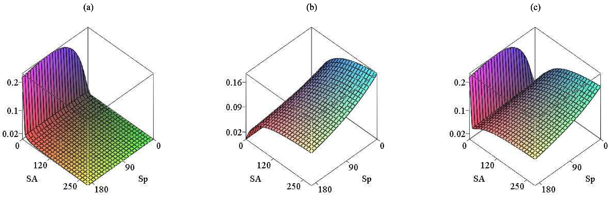
Figure 1 visualizes the functions ${\mu }_P(S_P,S_A)$, ${\mu }_A(S_P,S_A)$ and ${\mu }_P(S_P,S_A)+{\mu }_A(S_P,S_A)$.

The explicit expressions of ${\mu }_P$ and ${\mu }_A$ (see (4)) suggest the following properties of the latter:

Property 1. 

For $S_P\ge 0$, $S_A\ge 0$, ${\mu }_P(S_P,S_A)\ge 0$ with ${\mu }_P(S_P,S_A)>0$ if $S_P>0$, $S_A>0$; ${\mu }_P(S_P,S_A)$ is continuously differentiable and bounded;

$$\frac{\partial }{\partial S_A}{\mu }_P(S_P,S_A)<0,\underset{S_P\to \infty }{lim}{\mu }_P(S_P,S_A)=0,\underset{S_A\to \infty }{lim}{\mu }_P(S_P,S_A)=0.$$

Property 2. 

For $S_P\ge 0$, $S_A\ge 0$, ${\mu }_A(S_P,S_A)\ge 0$ with ${\mu }_A(S_P,S_A)>0$ if $S_P>0$, $S_A>0$; ${\mu }_A(S_P,S_A)$ is continuously differentiable and bounded;

$$\frac{\partial }{\partial S_P}{\mu }_A(S_P,S_A)<0,\underset{S_P\to \infty }{lim}{\mu }_A(S_P,S_A)=0,\underset{S_A\to \infty }{lim}{\mu }_A(S_P,S_A)=0.$$

3. Local Stability Analysis

In this section we investigate existence and local asymptotic stability of equilibrium points for model (1)–(3) in dependance of the key control parameter, the dilution rate D.

3.1. Existence of Equilibrium Points

The equilibrium points (called also steady states) are the simplest solutions of the dynamical system, which do not depend on time. Their existence is an essential prerequisite for global stabilization of the dynamics.

For model (1)–(3), the equilibrium points are solutions with respect to $(S_P,S_A,X)$ of the following system of nonlinear algebraic equations

$$\begin{array}{ccc}& & D(S_P^0-S_P)-{\displaystyle \frac{1}{Y_P}}{\mu }_P(S_P,S_A)X=0\hfill \end{array}$$

(5)

$$\begin{array}{ccc}& & D(S_A^0-S_A)-{\displaystyle \frac{1}{Y_A}}{\mu }_A(S_P,S_A)X=0\hfill \end{array}$$

(6)

$$\begin{array}{ccc}& & \left({\mu }_P(S_P,S_A)+{\mu }_A(S_P,S_A)-D\right)X=0.\hfill \end{array}$$

(7)

Obviously, $S_P=S_P^0$, $S_A=S_A^0$ and $X=0$ are solutions of (5)–(7) for any $D>0$. We denote this equilibrium point by $E_0=(S_P^0,S_A^0,0)$, which is called boundary or washout equilibrium.

Further we are looking for solutions of (5)–(7) with positive components. After multiplying Equation (5) by $Y_P$, Equation (6) by $Y_A$, summing the latter together and adding them to (7) we obtain the following expression for X

$$X=Y_P(S_P^0-S_P)+Y_A(S_A^0-S_A).$$

(8)

Obviously, $X>0$ will be valid if and only if $S_P<S_P^0$ and $S_A<S_A^0$ are satisfied.

Substituting X from (8) into Equations (5) and (6) leads to the following nonlinear algebraic system with respect to $S_P$ and $S_A$

$$\begin{array}{ccc}& & {\mu }_P(S_P,S_A)+{\mu }_A(S_P,S_A)=D\hfill \end{array}$$

(9)

$$\begin{array}{ccc}& & Y_P{\mu }_A(S_P,S_A)(S_P^0-S_P)-Y_A{\mu }_P(S_P,S_A)(S_A^0-S_A)=0.\hfill \end{array}$$

(10)

It follows from (9) that ${\mu }_A(S_P^0,S_A^0)+{\mu }_P(S_P^0,S_A^0)=D$, and then Equation (8) implies $X=0$. Denote

$$D_{max}={\mu }_A(S_P^0,S_A^0)+{\mu }_P(S_P^0,S_A^0).$$

(11)

The value $D_{max}$ will serve in the following as a critical point of the parameter D for existence of interior (with positive components) equilibrium points and for their local asymptotic stability.

The system (9) and (10) is difficult to be solved analytically due to the strong nonlinearities in the functions ${\mu }_A(S_P,S_A)$ and ${\mu }_P(S_P,S_A)$ with respect to $S_P$ and $S_A$. We shall show numerically that only one interior equilibrium exists for $D\in \left(0,D_{max}\right)$. Using the numerical values in Table 1 we get

$$D_{max}=0.0923920518.$$

We construct a mesh of points $\left\{D_j\right\}$ in the interval $\left(0,D_{max}\right]$ and for each value $D=D_j$ the system (9) and (10) is solved numerically, looking for solutions such that $0<S_P\le S_P^0$, $0<S_A\le S_A^0$. The third component X of the interior equilibrium is obtained from Equation (8). The numerical computations deliver existence of only one interior equilibrium point $E^{\ast }=E^{\ast }\left(D\right)=(S_P^{\ast },S_A^{\ast },X^{\ast })$. Figure 2 visualizes the components with respect to $S_P$, $S_A$ and X of the two equilibria $E^{\ast }$ and $E_0$. It is seen, that at $D=D_{max}$ the two equilibria $E^{\ast }$ and $E_0$ coincide, i.e., $S_P^{\ast }=S_P^0$, $S_A^{\ast }=S_A^0$ and $X^{\ast }=0$.

3.2. Local Asymptotic Stability of the Equilibrium Points

The local asymptotic stability of an equilibrium point is determined by the signs of the real parts of the eigenvalues of the Jacobian matrix evaluated at this equilibrium, or equivalently by the roots of the corresponding characteristic polynomial (cf. e.g., [18,40]).

The Jacobian matrix J related to the model Equations (1)–(3) has the form

$$J(S_P,S_A,X)=\left(\begin{array}{ccc}-D-\frac{1}{Y_P}\frac{\partial {\mu }_P}{\partial S_P}X\hfill & -\frac{1}{Y_A}\frac{\partial {\mu }_P}{\partial S_A}X\hfill & -\frac{1}{Y_P}{\mu }_P\hfill \\ -\frac{1}{Y_A}\frac{\partial {\mu }_A}{\partial S_P}X\hfill & -D-\frac{1}{Y_A}\frac{\partial {\mu }_A}{\partial S_A}X\hfill & -\frac{1}{Y_A}{\mu }_A\hfill \\ \left(\frac{\partial {\mu }_P}{\partial S_P}+\frac{\partial {\mu }_A}{\partial S_P}\right)X\hfill & \left(\frac{\partial {\mu }_P}{\partial S_A}+\frac{\partial {\mu }_A}{\partial S_A}\right)X\hfill & {\mu }_P+{\mu }_A-D\hfill \end{array}\right).$$

Denote by $|J\left(E_0\right)-\lambda I_3|$ the characteristic polynomial of J evaluated at the boundary equilibrium $E_0=(S_P^0,S_A^0,0)$. Here $I_3$ is the 3-dimensional identity matrix and $\lambda$ is any complex number. We obtain

$$\begin{array}{ccc}\hfill |J\left(E_0\right)-\lambda I_3\left)\right|& =& \left|\begin{array}{ccc}-D-\lambda \hfill & 0\hfill & -\frac{1}{Y_P}{\mu }_P(S_P^0,S_A^0)\hfill \\ 0\hfill & -D-\lambda \hfill & -\frac{1}{Y_A}{\mu }_A(S_P^0,S_A^0)\hfill \\ 0\hfill & 0\hfill & {\mu }_P(S_P^0,S_A^0)+{\mu }_A(S_P^0,S_A^0)-D-\lambda \hfill \end{array}\right|\hfill \\ & =& {(-D-\lambda )}^2({\mu }_P(S_P^0,S_A^0)+{\mu }_A(S_P^0,S_A^0)-D-\lambda ).\hfill \end{array}$$

Obviously, ${\lambda }_{1,2}=-D<0$ are two negative roots of the above characteristic polynomial. The third root is ${\lambda }_3={\mu }_P(S_P^0,S_A^0)+{\mu }_A(S_P^0,S_A^0)-D$. Since $D_{max}={\mu }_P(S_P^0,S_A^0)+{\mu }_A(S_P^0,S_A^0)$, the sign of ${\lambda }_3$ satisfies

$${\lambda }_3={\mu }_P(S_P^0,S_A^0)+{\mu }_A(S_P^0,S_A^0)-D\left\{\begin{array}{cc}>0,\hfill & \mathrm{if} D<D_{max},\hfill \\ <0,\hfill & \mathrm{if} D>D_{max},\hfill \\ =0,\hfill & \mathrm{if} D=D_{max}.\hfill \end{array}\right.$$

Therefore

$$E_0 \mathrm{is}\left\{\begin{array}{cc}\mathrm{locally} \mathrm{asymptotically} \mathrm{unstable},\hfill & \mathrm{if} D<D_{max},\hfill \\ \mathrm{locally} \mathrm{asymptotically} \mathrm{stable},\hfill & \mathrm{if} D>D_{max}.\hfill \end{array}\right.$$

At $D=D_{max}$ the third eigenvalue ${\lambda }_3$ becomes equal to zero, so $E_0$ can undergo a bifurcation at this value of D.

The eigenvalues of the interior equilibrium $E^{\ast }$ are determined numerically, using the already computed values of the equilibrium components on the mesh $\left\{D_j\right\}$. Figure 3 visualizes the three eigenvalues of $E^{\ast }$ with respect to D. It is seen, that the three eigenvalues of $E^{\ast }$ are negative for $D<D_{max}$, thus the interior equilibrium is locally asymptotically stable. At $D=D_{max}$ the first eigenvalue approaches zero, so $E^{\ast }$ undergoes a local bifurcation. In fact, $E_0$ and $E^{\ast }$ coalesce at $D=D_{max}$ and exchange stability, thus a transcritical bifurcation occurs at this value of D.

We summarize the above results in the following assertion.

Proposition 1. 

(i) 

The model (1)–(3) possesses a boundary equilibrium $E_0=(S_P^0,S_A^0,0)$ (with $X=0$) for all values of the dilution rate $D>0$. There exists a critical value $D_{max}>0$ of the dilution rate D, such that $E_0$ is locally asymptotically stable for $D>D_{max}$, and $E_0$ is locally asymptotically unstable for $0<D<D_{max}$.

(ii) 

An interior equilibrium $E^{\ast }=(S_P^{\ast },S_A^{\ast },X^{\ast })>0$ exists and is locally asymptotically stable for all $D\in (0,D_{max})$.

(iii) 

At $D=D_{max}$ the two equilibrium points $E_0$ and $E^{\ast }$ undergo a transcritical bifurcation, leading to stability exchange between them.

4. Global Analysis

In this section we provide the most important properties of the dynamics (1)–(3). We establish existence and positivity of the solutions for all time $t\ge 0$—properties, that ensure the ability of the mathematical model to describe the bioprocess, regarding its practical applicability. Further, we show the global asymptotic stability of the equilibrium points with respect to the dilution rate D, which actually means model-based control design of the process. These results provide a good framework for practical applications by indicating to the experimenter how to choose the proper control strategy in order to ensure best process performance and wastewater depollution up to known ecological norms.

Theorem 1. 

The nonnegative cone and the interior of the nonnegative cone in ${\mathbb{R}}^3$ are positively invariant under the flow (1)–(3).

Proof. 

If $X\left(\tau \right)=0$ at some time moment $\tau \ge 0$ then by Equation (3) it follows $X\left(t\right)=0$ for all $t\ge 0$ due to uniqueness of solutions of Cauchy’s problem. Then the model reduces to

$$\begin{array}{ccc}\hfill {\displaystyle \frac{d{S}_P\left(t\right)}{dt}}& =& D(S_P^0-S_P\left(t\right))\hfill \\ \hfill {\displaystyle \frac{d{S}_A\left(t\right)}{dt}}& =& D(S_A^0-S_A\left(t\right)),\hfill \end{array}$$

which solutions are

$$\begin{array}{ccc}\hfill S_P\left(t\right)& =& S_P^0+(S_P^0-S_P\left(0\right))e^{-Dt}\hfill \\ \hfill S_A\left(t\right)& =& S_A^0+(S_A^0-S_A\left(0\right))e^{-Dt}.\hfill \end{array}$$

Obviously, $S_P\left(t\right)\to S_P^0$ and $S_A\left(t\right)\to S_A^0$ exponentially as $t\to \infty$. So, the face $\{S_P\ge 0,S_A\ge 0,X=0\}$ is invariant under the flow (1)–(3).

If $X\left(0\right)>0$ then it follows from Equation (3)

$$X\left(t\right)=X\left(0\right)e^{{\int }_0^t[{\mu }_P(S_P\left(\theta \right),S_A\left(\theta \right))+{\mu }_A(S_P\left(\theta \right),S_A\left(\theta \right))-D]d\theta },$$

which means that $X\left(t\right)>0$ for all $t>0$.

If $S_P\left(\tau \right)=0$ for some $\tau \ge 0$ then by Equation (1), ${\displaystyle \frac{d{S}_P\left(t\right)}{dt}}=D{S}_P^0>0$. If $S_A\left(\tau \right)=0$ for some $\tau \ge 0$ then Equation (2) implies ${\displaystyle \frac{d{S}_A\left(t\right)}{dt}}=D{S}_A^0>0$. Therefore the vector field of (1)–(3) points inside the positive orthant, i.e., all model solutions are positive. This completes the proof of Theorem 1. □

In what follows we shall consider initial conditions for the dynamics (1)–(3) in the set

$$\Omega =\left\{(S_P,S_A,X):S_P\left(0\right)>0,S_A\left(0\right)>0,X\left(0\right)>0\right\}.$$

According to Theorem 1 the set $\Omega$ is positively invariant for the model, i.e., starting with initial conditions in $\Omega$ the corresponding solutions remain in $\Omega$ for all time $t\ge 0$.

Theorem 2. 

Let $(S_P\left(0\right),S_A\left(0\right),X\left(0\right))\in \Omega$. Then all solutions are uniformly bounded and thus exist for all time $t>0$.

Proof. 

After multiplying Equation (1) by $Y_P$, Equation (2) by $Y_A$ and adding the latter to Equation (3) we obtain

$$\begin{array}{c}{\displaystyle Y_P{\displaystyle \frac{d{S}_P\left(t\right)}{dt}}+Y_A{\displaystyle \frac{d{S}_A\left(t\right)}{dt}}+{\displaystyle \frac{dX\left(t\right)}{dt}}}\hfill \\ =D\left[-\left(Y_P{S}_P\left(t\right)+Y_A{S}_A\left(t\right)+X\left(t\right)\right)+Y_P{S}_P^0+Y_A{S}_A^0\right].\hfill \end{array}$$

(12)

Denoting $Z\left(t\right)=Y_P{S}_P\left(t\right)+Y_A{S}_A\left(t\right)+X\left(t\right)$, Equation (12) implies

$${\displaystyle \frac{dZ\left(t\right)}{dt}}=D\left(-Z\left(t\right)+Y_P{S}_P^0+Y_A{S}_A^0\right),$$

which yields ${lim}_{t\to \infty }Z\left(t\right)=Y_P{S}_P^0+Y_A{S}_A^0$. According to Theorem 1 all solutions are positive, and the latter presentation means that all solutions are uniformly bounded and thus exist for all $t>0$. The proof of Theorem 2 is completed. □

In the following we shall use the next Lemma.

Barbălat’s Lemma 

(cf. [41]). If $f:(0,\infty )\to \mathbb{R}$ is uniformly continuous and there exists ${\displaystyle \underset{t\to \infty }{lim}{\int }_0^{t}f\left(\xi \right)d\xi }$ then ${\displaystyle \underset{t\to \infty }{lim}f\left(t\right)=0}$.

Theorem 3. 

Let $(S_P\left(0\right),S_A\left(0\right),X\left(0\right))\in \Omega$. The following assertions are valid.

(i) 

For any $D>0$ and for any $\epsilon >0$ there exists time $T_{\epsilon }>0$ such that for all $t>T_{\epsilon }$, $S_P\left(t\right)\le S_P^0+\epsilon$ and $S_A\left(t\right)\le S_A^0+\epsilon$ hold true.

(ii) 

If $D\in (0,D_{max})$, then there exists time $T>0$ such that for all $t>T$, $S_P\left(t\right)<S_P^0$ and $S_A\left(t\right)<S_A^0$ are fulfilled.

Proof. 

$\left(i\right)$ Let $D>0$ be any value of the control function. If $S_P\left(t\right)>S_P^0$ holds for all $t\ge 0$ then by Equation (1) we obtain ${\displaystyle \frac{d{S}_P\left(t\right)}{dt}}<0$ for all $t>0$. If there is a time moment $\tilde{t}>0$ such that $S_P\left(\tilde{t}\right)=S_P^0$ then ${\displaystyle \frac{d{S}_P\left(\tilde{t}\right)}{dt}}=-{\displaystyle \frac{1}{Y_P}}{\mu }_P(S_P\left(\tilde{t}\right),S_A\left(\tilde{t}\right))X\left(\tilde{t}\right)<0$. This means that if there is a time moment ${\tilde{t}}_1>0$ such that $S_P\left({\tilde{t}}_1\right)\le S_P^0$ then $S_P\left(t\right)<S_P^0$ for all $t>{\tilde{t}}_1$ is valid. Therefore, $S_P\left(t\right)$ converges to some ${\tilde{S}}_P\ge S_P^0$ as $t\to \infty$. If ${\tilde{S}}_P>S_P^0$ then ${\displaystyle \frac{d{S}_P\left(t\right)}{dt}}<(S_P^0-{\tilde{S}}_P)D<0$ for all $t>0$, which means that $S_P\left(t\right)\to -\infty$ as $t\to \infty$, a contradiction. Thus, either $S_P\left(t\right)\le S_P^0$ for all sufficiently large $t>0$ or $S_P\left(t\right)$ converges to $S_P^0$ as $t\to \infty$. Hence, for any $\epsilon >0$ there exists time $T_P>0$ such that $S_P\left(t\right)<S_P^0+\epsilon$ for all $t>T_P$ holds true.

Similar conclusion can be made for $S_A\left(t\right)$ using the model Equation (2), i.e., either $S_A\left(t\right)\le S_A^0$ for all sufficiently large $t>0$ or $S_A\left(t\right)$ converges to $S_A^0$ as $t\to \infty$. Equivalently, for any $\epsilon >0$ there exists time $T_A>0$ so that for all $t\ge T_A$ the inequality $S_A\left(t\right)\le S_A^0+\epsilon$ holds true. Then choosing $T_{\epsilon }=max\{T_P,T_A\}$ proves point $\left(i\right)$ of the theorem.

$\left(ii\right)$ Choose and fix some $\overline{D}\in (0,D_{max})$. The proof of point $\left(i\right)$ implies that $S_P\left(t\right)$ is strictly decreasing with time. Moreover, since the set $\{S_P\left(t\right):t\in [0,+\infty )\}$ is bonded, it follows that there exists ${lim}_{t\to \infty }{S}_P\left(t\right)$. Similarly, $S_A\left(t\right)$ is strictly decreasing, too, and there exists ${lim}_{t\to \infty }{S}_A\left(t\right)$. Since $S_P\left(t\right)$, $S_A\left(t\right)$ and $X\left(t\right)$ are bounded differentiable functions for all $t\in (0,+\infty )$ it follows that ${\displaystyle \frac{d{S}_P\left(t\right)}{dt}}$ is uniformly continuous. Applying Barbălat’s Lemma yields

$$0=\underset{t\to \infty }{lim}{\displaystyle \frac{d}{dt}}{S}_P\left(t\right)=\underset{t\to \infty }{lim}\left(\overline{D}(S_P^0-S_P\left(t\right))-{\displaystyle \frac{1}{Y_P}}{\mu }_P(S_P\left(t\right),S_A\left(t\right))X\left(t\right)\right).$$

(13)

We have by Theorem 1 that $S_P\left(t\right)>0$, $S_A\left(t\right)>0$, $X\left(t\right)>0$, and because ${\mu }_P(S_P,S_A)>0$, the latter equality (13) implies $S_P\left(t\right)\downarrow S_P^0$, $X\left(t\right)\downarrow 0$ as $t\to \infty$. In a similar way one obtains that $S_A\left(t\right)\downarrow S_A^0$ as $t\to \infty$.

Since $\overline{D}<D_{max}={\mu }_P(S_P^0,S_A^0)+{\mu }_A(S_P^0,S_A^0)$, by Equation (3) we obtain

$$\begin{array}{ccc}\hfill {\displaystyle \frac{dX\left(t\right)}{dt}}& =& ({\mu }_P(S_P\left(t\right),S_A\left(t\right))+{\mu }_A(S_P\left(t\right),S_A\left(t\right))-\overline{D})X\left(t\right)\hfill \\ & >& \left({\mu }_P(S_P\left(t\right),S_A\left(t\right))+{\mu }_A(S_P\left(t\right),S_A\left(t\right))-D_{max}\right)X\left(t\right).\hfill \end{array}$$

Further, the relations $S_P\left(t\right)\downarrow S_P^0$, $S_A\left(t\right)\downarrow S_A^0$ as $t\to \infty$, as well as the properties $\left(P1\right)$, $\left(P2\right)$ of ${\mu }_P(·)$ and ${\mu }_A(·)$ imply that there exists a time moment $\overline{t}$ and a constant $\gamma >0$ such that

$${\mu }_P(S_P\left(t\right),S_A\left(t\right))+{\mu }_A(S_P\left(t\right),S_A\left(t\right))-D_{max}\ge \gamma$$

for all $t>\overline{t}$ is fulfilled. Then ${\displaystyle \frac{dX\left(t\right)}{dt}}\ge \gamma X\left(t\right)>0$ for all $t>\overline{t}$. The invariance of $\Omega$ with respect to the trajectories of the system implies that $X\left(\overline{t}\right)>0$. Then from ${\displaystyle \frac{dX\left(t\right)}{dt}}>0$ for all $t>\overline{t}$ it follows that $X\left(t\right)>X\left(\overline{t}\right)$ for each $t>\overline{t}$, a contradiction with $X\left(t\right)\downarrow 0$ as $t\to \infty$. Hence, there exists a sufficiently large time $T_P>0$ such that $S_P\left(t\right)\le S_P^0$ holds true for all $t>T_P$. If for some time moment $\widehat{t}>T_P$ the equality $S_P\left(\widehat{t}\right)=S_P^0$ is fulfilled, then

$${\displaystyle \frac{d{S}_P\left(\widehat{t}\right)}{dt}}=-{\displaystyle \frac{1}{Y_P}}{\mu }_P(S_P\left(\widehat{t}\right),S_A\left(\widehat{t}\right))X\left(\widehat{t}\right)<0.$$

This shows that $S_P\left(t\right)<S_P^0$ for all sufficiently large $t>T_P$ is satisfied.

In a similar way it can be shown that there exists time $T_A>0$ such that $S_A\left(t\right)<S_A^0$ for all $t>T_A$ holds true. Choosing $T=max\{T_P,T_A\}$ it follows that $S_P\left(t\right)<S_P^0$ and $S_A\left(t\right)<S_A^0$ are simultaneously satisfied for all $t>T$.

The proof of Theorem 3 is completed. □

Below we shall establish the global asymptotic stability of the boundary equilibrium $E_0$. This property of the washout steady state is also important because it characterizes the inability of the microorganisms to survive in the chemostat system and to degrade the organic chemical compounds.

Theorem 4. 

For any initial point from Ω and any $D>D_{max}$ the corresponding solution of (1)–(3) converges asymptotically to the boundary equilibrium $E_0=(S_P^0,S_A^0,0)$.

Proof. 

Choose an arbitrary initial point $(S_P\left(0\right),S_A\left(0\right),X\left(0\right))\in \Omega$, and let $\overline{D}>D_{max}$ be some value of the dilution rate. Suppose that ${lim}_{t\to \infty }X\left(t\right)=\overline{X}>0$. By Barbălat’s Lemma we obtain from Equation (3)

$$0=\underset{t\to \infty }{lim}\frac{d}{dt}X\left(t\right)=\underset{t\to \infty }{lim}\left[{\mu }_P(S_P\left(t\right),S_A\left(t\right))+{\mu }_A(S_P\left(t\right),S_A\left(t\right))-\overline{D}\right]\overline{X},$$

which leads to

$$\underset{t\to \infty }{lim}\left[{\mu }_P(S_P\left(t\right),S_A\left(t\right))+{\mu }_A(S_P\left(t\right),S_A\left(t\right))\right]=\overline{D}>D_{max}.$$

Based on Theorem 3$\left(i\right)$, on the properties $\left(P1\right)$ and $\left(P2\right)$ of ${\mu }_P(·)$ and ${\mu }_A(·)$, and since $D_{max}={\mu }_P(S_P^0,S_A^0)+{\mu }_A(S_P^0,S_A^0)$, the latter relation implies that there exists a time moment $\widehat{t}>0$ and a constant $\delta >0$ such that

$${\mu }_P(S_P\left(t\right),S_A\left(t\right))+{\mu }_A(S_P\left(t\right),S_A\left(t\right))-\overline{D}\ge \delta$$

for all $t>\widehat{t}$. This yields ${\displaystyle \frac{d}{dt}}X\left(t\right)\ge \delta X\left(t\right)$, or equivalently, $X\left(t\right)\ge X\left(\widehat{t}\right)e^{\delta (t-\widehat{t})}$ for all $t>\widehat{t}$, a contradiction with ${lim}_{t\to \infty }X\left(t\right)=\overline{X}$. Hence, ${lim}_{t\to \infty }X\left(t\right)=0$ holds true. Further, applying the theory of the asymptotically autonomous systems, the model (1)–(3) reduces to the limiting system

$${\displaystyle \frac{d}{dt}}{S}_P\left(t\right)=\overline{D}(S_P^0-S_P\left(t\right)),{\displaystyle \frac{d}{dt}}{S}_A\left(t\right)=\overline{D}(S_A^0-S_A\left(t\right)),$$

which means that ${lim}_{t\to \infty }{S}_P\left(t\right)=S_P^0$, ${lim}_{t\to \infty }{S}_A\left(t\right)=S_A^0$. This proves the global asymptotic stability of the washout equilibrium $E_0$. □

The next considerations concern the global asymptotic stability of the interior equilibrium $E^{\ast }=(S_P^{\ast },S_A^{\ast },X^{\ast })$ whenever $D\in (0,D_{max})$.

Experimental results in [16] indicate that SA is degraded more rapidly by P. putida 49451 cells than phenol. For that reason let us assume that the model dynamics is already stabilized at $S_A^{\ast }<S_A^0$ for some value $D^{\ast }\in (0,D_{max})$. Denote

$$C_A^{\ast }=Y_A(S_A^0-S_A^{\ast }).$$

(14)

Then model (1)–(3) can be reduced to the following 2-dimensional system with respect to $S_P$ and X:

$$\begin{array}{ccc}\hfill {\displaystyle \frac{d{S}_P\left(t\right)}{dt}}& =& D^{\ast }(S_P^0-S_P\left(t\right))-{\displaystyle \frac{1}{Y_P}}{\mu }_P(S_P\left(t\right),S_A^{\ast })X\left(t\right)\hfill \\ \hfill {\displaystyle \frac{dX\left(t\right)}{dt}}& =& \left({\mu }_P(S_P\left(t\right),S_A^{\ast })-D^{\ast }\right)X\left(t\right)+C_A^{\ast }{D}^{\ast }.\hfill \end{array}$$

Further, by (9) and (10) we have $S_P^0=S_P^{\ast }+{\displaystyle \frac{1}{Y_P}}(X^{\ast }-S_P^{\ast })+C_A^{\ast }$, and the above two equations can be rewritten in the form

$$\begin{array}{ccc}{\displaystyle \frac{d{S}_P\left(t\right)}{dt}}\hfill & =& -D^{\ast }\left[S_P\left(t\right)-S_P^{\ast }+{\displaystyle \frac{1}{Y_P}}(X\left(t\right)-X^{\ast })\right]-{\displaystyle \frac{1}{Y_P}}{C}_A^{\ast }{D}^{\ast }\hfill \\ \hfill & & -{\displaystyle \frac{1}{Y_P}}({\mu }_P(S_P\left(t\right),S_A^{\ast })-D^{\ast })X\left(t\right)\hfill \\ {\displaystyle \frac{dX\left(t\right)}{dt}}\hfill & =& \left({\mu }_P(S_P\left(t\right),S_A^{\ast })-D^{\ast }\right)X\left(t\right)+C_A^{\ast }{D}^{\ast }.\hfill \end{array}$$

(15)

We shall show that the dynamics (15) is asymptotically stabilizable towards $(S_P^{\ast },X^{\ast })$.

Theorem 5. 

For any initial point $(S_P\left(0\right),X\left(0\right))>0$ the corresponding solution $(S_P\left(t\right),X\left(t\right))$ of (15) converges asymptotically to $(S_P^{\ast },X^{\ast })$.

Proof. 

From Theorem 3$\left(ii\right)$ it follows that there is no loss of generality if we restrict our considerations to initial conditions from the set

$${\Omega }_1=\{(S_P,X):0<S_P\left(0\right)<S_P^0,X>0\}.$$

Define the following Lyapunov function

$$V=V(S_P,X)={\left(S_P-S_P^{\ast }+{\displaystyle \frac{1}{Y_P}}(X-X^{\ast })\right)}^2+\Gamma {\int }_{S_P^{\ast }}^{S_P}{\displaystyle \frac{v-S_P^{\ast }}{S_P^0-v}}dv,$$

where $\Gamma$ is a positive constant, which will be determined later. Obviously, V is continuously differentiable in $\Omega$, $V>0$ for all $(S_P,X)\in {\Omega }_1$ with $S_P<S_P^0$, and $V=0$ at $(S_P^{\ast },X^{\ast })$. It is straightforward to see, that the derivative of V along the solutions of (15) is

$$\begin{array}{ccc}\hfill {\displaystyle \frac{dV}{dt}}& =& 2\left(S_P-S_P^{\ast }+\frac{1}{Y_P}(X-X^{\ast })\right)·\left(\frac{d{S}_P}{dt}+\frac{1}{Y_P}\frac{dX}{dt}\right)+\Gamma {\displaystyle \frac{S_P-S_P^{\ast }}{S_P^0-S_P}}·\frac{d{S}_P}{dt}\hfill \\ & =& -2D^{\ast }{\left[S_P-S_P^{\ast }+\frac{1}{Y_P}(X-X^{\ast })\right]}^2\hfill \\ & & -\Gamma {\displaystyle \frac{1}{S_P^0-S_P}}\left[{(S_P-S_P^{\ast })}^2+\frac{1}{Y_P}(S_P-S_P^{\ast })(X-X^{\ast })\right]\hfill \\ & & -\Gamma {\displaystyle \frac{1}{S_P^0-S_P}}\left[\frac{1}{Y_P}{C}_A^{\ast }(S_P-S_P^{\ast })+\frac{1}{Y_P}({\mu }_P(S_P,S_A^{\ast })-D^{\ast })X(S_P-S_P^{\ast })\right]\hfill \\ & =& -\left(2D^{\ast }+{\displaystyle \frac{\Gamma }{S_P^0-S_P}}\right){(S_P-S_P^{\ast })}^2-2D^{\ast }{\displaystyle \frac{1}{Y_P^2}}{(X-X^{\ast })}^2\hfill \\ & & -\left(4D^{\ast }\frac{1}{Y_P}+{\displaystyle \frac{\Gamma }{Y_P(S_P^0-S_P)}}\right)(S_P-S_P^{\ast })(X-X^{\ast })\hfill \\ & & -\Gamma {\displaystyle \frac{1}{Y_P}}·{\displaystyle \frac{S_P-S_P^{\ast }}{S_P^0-S_P}}\left(C_A^{\ast }+({\mu }_P(S_P,S_A^{\ast })-D^{\ast })X\right).\hfill \end{array}$$

Since all model solutions are positive and bounded, we can choose the constant $\Gamma >0$ sufficiently large so that ${\displaystyle \frac{dV}{dt}}\le 0$ for all $(S_P,X>0)\in {\Omega }_1$. Obviously, ${\displaystyle \frac{dV}{dt}}=0$ if and only if $S_P=S_P^{\ast }$ and $X=X^{\ast }$ are fulfilled. By LaSalle’s invariance principle (cf. [42]) every solution of (15) initiating in ${\Omega }_1$ approaches the largest invariant set $V^{\ast }=\{(S_P,X):\frac{dV}{dt}=0\}$. Since $E^{\ast }$ is locally asymptotically stable, it follows that $V^{\ast }=\left\{(S_P^{\ast },X^{\ast })\right\}$. Therefore, $(S_P^{\ast },X^{\ast })$ is globally asymptotically stable for system (15), and this means that all solutions of (1)–(3) converge to $E^{\ast }=(S_P^{\ast },S_A^{\ast },X^{\ast })$ as $t\to \infty$. The proof of Theorem 5 is completed. □

Remark 1. 

Similar conclusions about the global stability of $E^{\ast }$ can be made by assuming that the dynamics is first stabilized at $S_P=S_P^{\ast }$ for some $D^{\ast }\in (0,D_{max})$ and then show that the solutions $(S_A\left(t\right),X\left(t\right))$ converge asymptotically to $(S_A^{\ast },X^{\ast })$ as $t\to \infty$. This will be in agreement with the experimental work in [14] where it is concluded that P. putida CCRC 14365 cells preferably degrade phenol rather than SA.

5. Numerical Simulation of the Model Dynamics

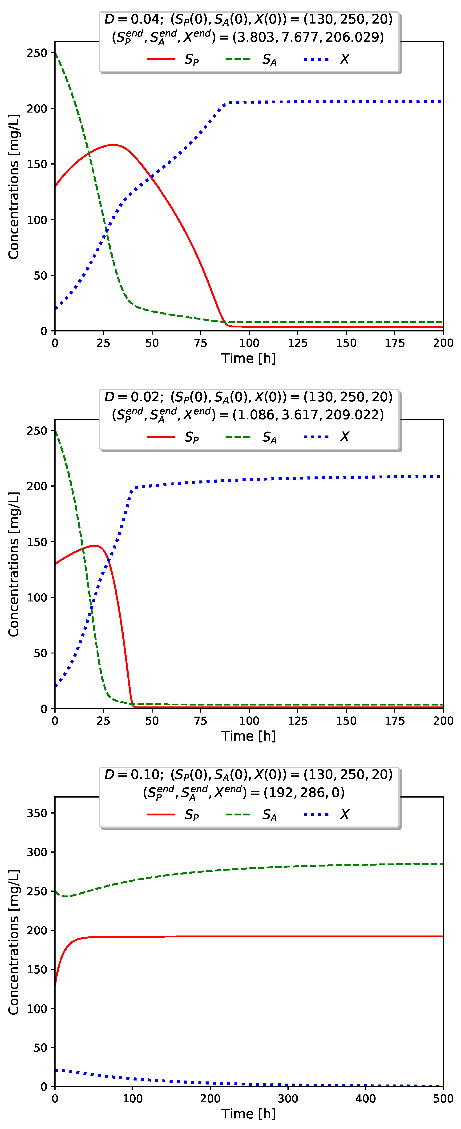
In this section we consider numerical examples demonstrating the dynamic behavior of the model (1)–(3) in accordance with the theoretical results.

Example 1. 

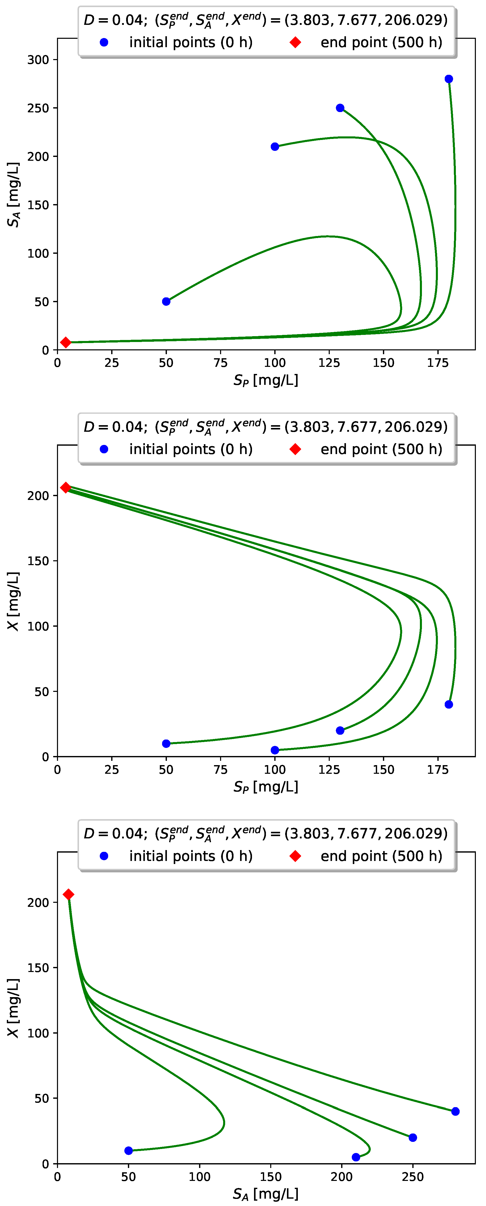
$D=0.04<D_{max}=0.0923920518$

As mentioned before, the model (1)–(3) has been tested at this value of D in [16]. It is shown there that the solutions fall in finite time into the point $F=(6.6,8.5,232)$, called a steady state, but it is not. Our computer simulations deliver the following components for the interior equilibrium $E^{\ast }=(S_P^{\ast },S_A^{\ast },X^{\ast })=(3.803,7.677,206.029)$, which are quite different from that ones of F. According to Theorem 5 namely the equilibrium $E^{\ast }$ is globally asymptotically stable and attracts all solutions for any initial point from the set $\Omega$ as time tends to infinity. Practically this means that after finite time the solutions fall into a neighborhood of $E^{\ast }$, say a ball with center $E^{\ast }$ and radius $r>0$, where the value r (called also tolerance) can be chosen by the user.

Example 2. 

$D=0.02$

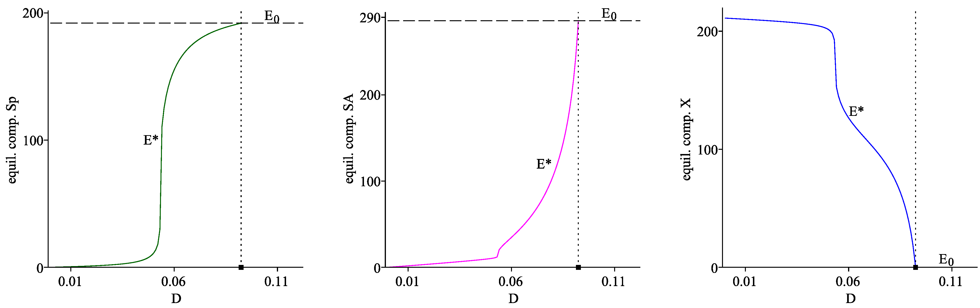
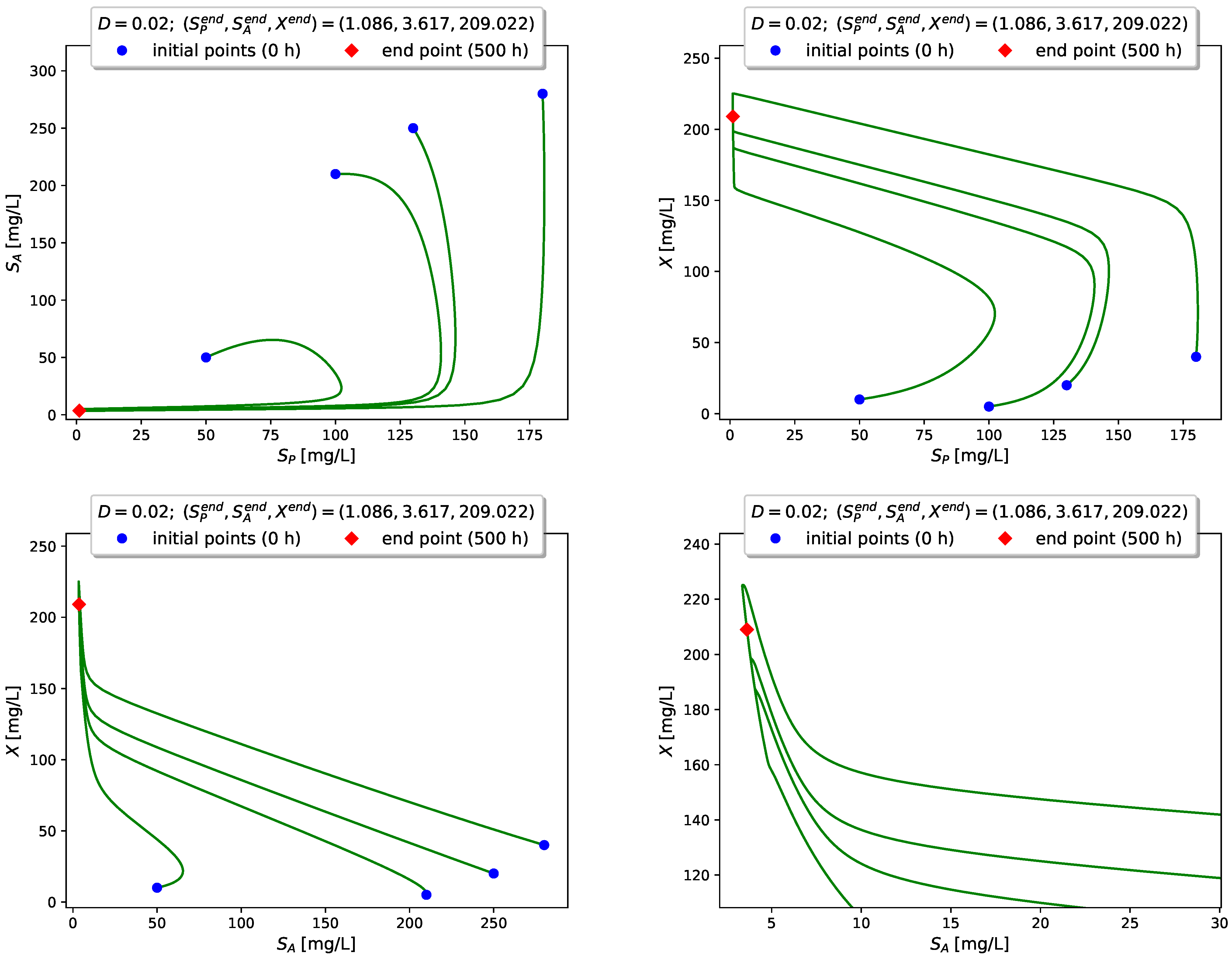
At $D=0.02<D_{max}$ the equilibrium components of the interior equilibrium are $E^{\ast }=(S_P^{\ast },S_A^{\ast },X^{\ast })=(1.086,3.617,209.022)$. Obviously, lower values of the dilution rate D lead to lower values of $S_P^{\ast }$ and $S_A^{\ast }$, but high values of $X^{\ast }$ in the global attractor $E^{\ast }$.

Example 3. 

$D=0.1$

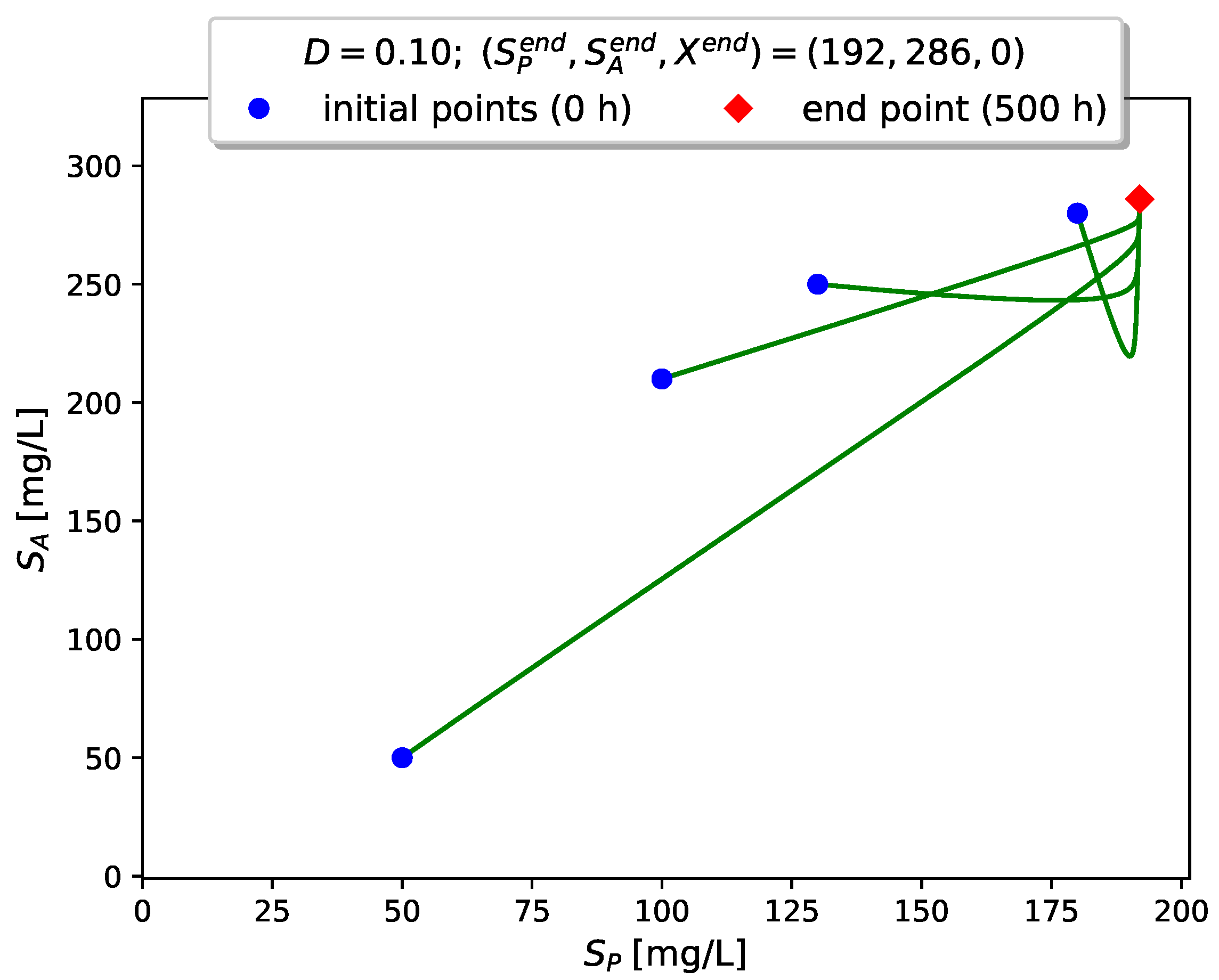
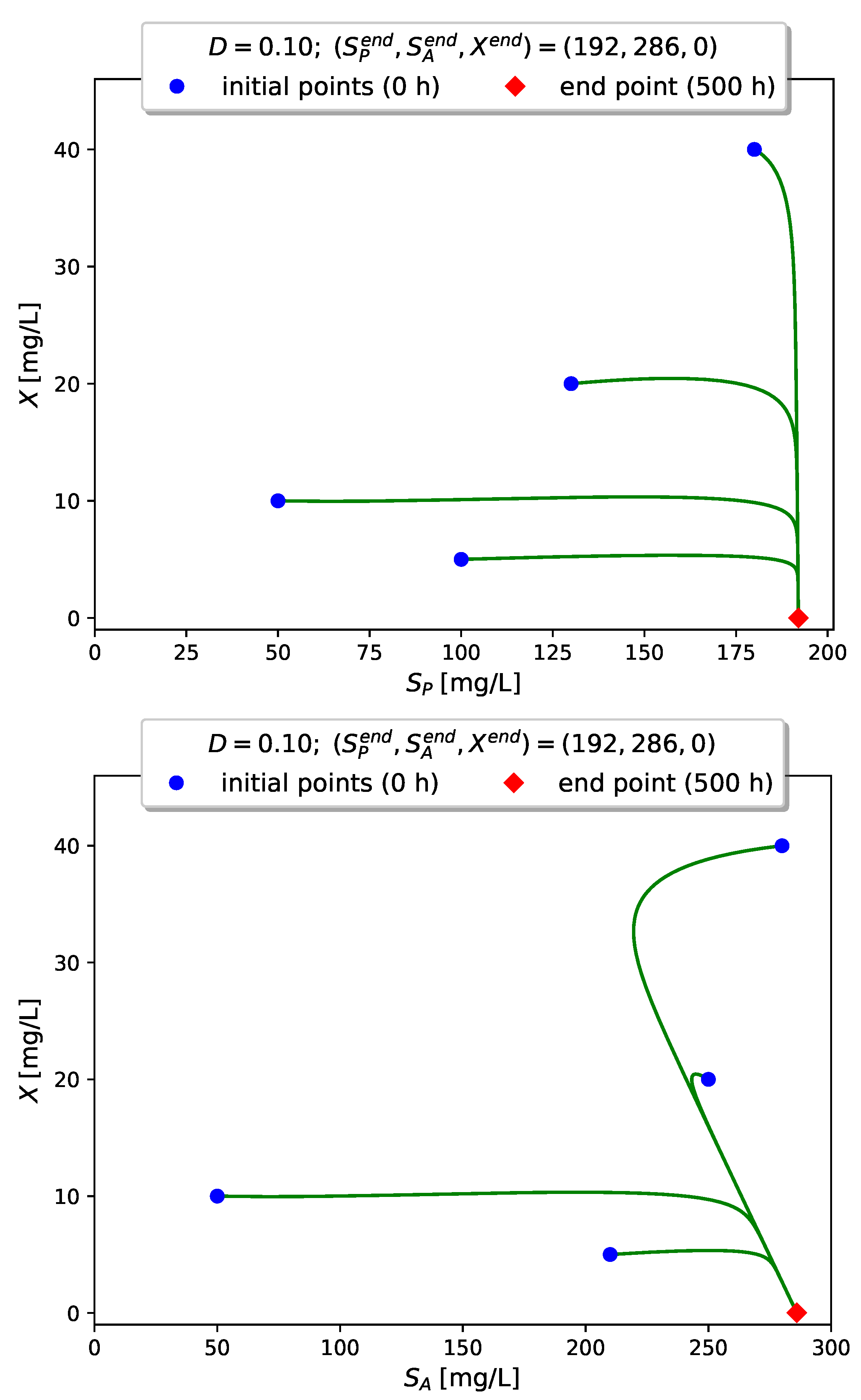
In this case we have $D>D_{max}=0.0923920518$, so that the boundary equilibrium $E_0=(S_P^0,S_A^0,0)=(192,286,0)$ is the unique global attractor of the model.

Figure 4 visualizes the time evolution of $S_P\left(t\right)$, $S_A\left(t\right)$ and $X\left(t\right)$ for the 3 different values of D corresponding to Examples 1–3.

Figure 5, Figure 6 and Figure 7 show projections of several trajectories in different phase planes for values of D according to Examples 1, 2 and 3, respectively.

The computer simulations with model (1)–(3) confirm the global stabilizability of the dynamics to either the interior (persistence) equilibrium $E^{\ast }$ if $0<D<D_{max}$ or to the boundary (washout) equilibrium $E_0$ when $D>D_{max}$.

6. Discussion and Conclusions

In this paper we provide a mathematical analysis of the model for biodegradation of phenol and sodium salicylate in a chemostat by P. putida 49451 cells, proposed for the first time and experimentally validated in [16]. The model is described by a system of three nonlinear ordinary differential equations involving SKIP kinetics as specific growth rate of the microorganisms. The mathematical investigation of the dynamical system includes local and global analysis of the solutions. Two equilibrium points—one interior (persistence) and one boundary (washout) equilibrium—are computed in dependance of the dilution rate D as an important model parameter. A critical value $D_{max}>0$ is found, such that the interior equilibrium point $E^{\ast }=(S_P^{\ast },S_A^{\ast },X^{\ast })$ exists if $0<D<D_{max}$. The boundary steady state $E_0=(S_P^0,S_A^0,0)$ is available for all values of $D>0$. It is shown by numerical computations that $E^{\ast }$ is locally asymptotically stable whenever it exists, and $E_0$ is locally asymptotically stable for $D>D_{max}$, and unstable if $D<D_{max}$. 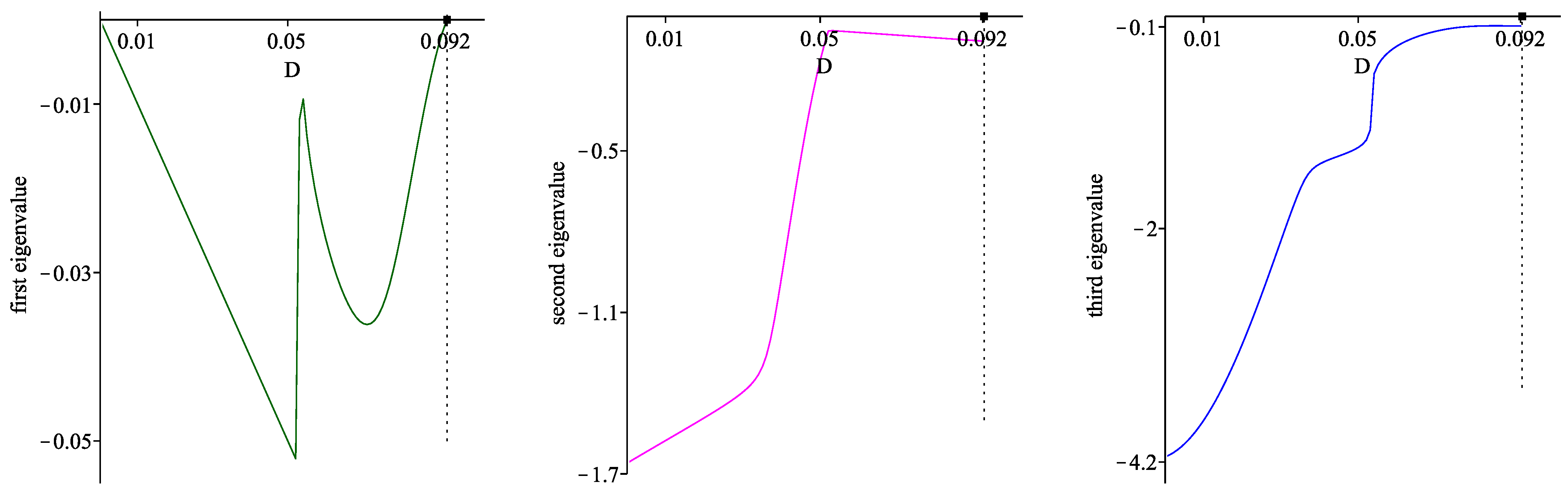These conclusions are summarized in Proposition 1.

The most important properties of the model solutions—existence, positivity, uniqueness and uniform boundedness—are established theoretically in Section 4, by Theorems 1–3. In Theorem 4 we prove the global stability of the boundary equilibrium $E_0=(S_P^0,S_A^0,0)$ (within $X=0$) if the values of the dilution rate D are large, i.e., if $D>D_{max}$. As usual, the global stability of $E_0$ is interpreted as total washout of the microorganisms from the chemostat leading to process breakdown. Theorem 5 is devoted to global stability of the interior equilibrium $E^{\ast }=(S_P^{\ast },S_A^{\ast },X^{\ast })$ for any $D\in (0,D_{max})$. The theorem is proved by assuming that the model dynamics is already stabilized to $S_A^{\ast }$ for some value $D^{\ast }\in (0, D_{max})$, and then it is shown, by providing an explicit Lyapunov function, that the solutions $S_P\left(t\right)$ and $X\left(t\right)$ converge asymptotically to $S_P^{\ast }$ and $X^{\ast }$ respectively as $t\to \infty$ for any initial point in the set $\Omega$. A similar result can be obtained supposing that the dynamics is first stabilized to $S_P^{\ast }$, and then showing that $S_A\left(t\right)\to S_A^{\ast }$ and $X\left(t\right)\to X^{\ast }$ respectively as $t\to \infty$ (see Remark 1). The global stability characteristics give useful advises to the experimenter how to tune the dilution rate D in order to control the biodegradation of the chemical compounds up to prescribed ecological norms.

It remains an open problem to prove the global asymptotic stability of the interior equilibrium $E^{\ast }$ with $D\in (0,D_{max})$ for the whole system (1)–(3), for example by constructing an appropriate Lyapunov function or using other approaches. This will be a subject of future studies.

Some numerical examples for different values of the dilution rate D support the theoretical studies and illustrate the dynamic behavior of the solutions. The model predictions are in agreement with the experimental work in [16] for phenol and SA biodegradation by P. putida cells.