Two-Dimensional Age Replacement Decision for Structural Dependence Parallel Systems via Intelligent Optimization Algorithm

Abstract

From large-scale aerospace systems to household appliances and other systems in daily life, the application of parallel systems is involved. A parallel system is a typical structural dependence multi-component system, in addition to a series system and hybrid system. This paper takes a parallel system as the research object and minimizes the expected cost rate or maximizes the availability by determining the optimal two-dimensional age replacement interval. The structural dependence of the components is described by the copula function, and the system life model is established. Based on the system life model, the two-dimensional age replacement expected cost rate model and availability model are proposed. In case analysis, the simulated annealing algorithm (SAA), genetic algorithm (GA) and particle swarm optimization (PSO) algorithm are used to find the optimal warranty scheme for the engine fuel fine filter. SAA can converge faster and find a warranty scheme that makes the warranty cost rate lower or the availability higher. Compared with one-dimensional age replacement, two-dimensional age replacement strategy has more advantages in saving warranty costs and improving system availability. Finally, rationalization suggestions are put forward for managers to make maintenance decisions through comparative analysis and sensitivity analysis.

1. Introduction

Periodic maintenance is a type of preventive maintenance strategy whose main goal is to prevent equipment failures from occurring before they occur [1]. In terms of the maintenance degree, periodic maintenance can be separated into four categories: deterioration maintenance, minimal maintenance, imperfect maintenance and perfect maintenance. The two most common maintenance methods are imperfect maintenance and perfect maintenance. Imperfect maintenance usually comprises activities such as equipment inspections, partial or full overhauls in a specific cycle, oil changes, lubrication, etc. Perfect maintenance usually utilizes replacements to enhance the reliability of equipment before it actually fails [2]. A periodic maintenance plan can prevent equipment failure and its serious consequences, but too frequent maintenance can result in increased maintenance costs or reduced system availability. Therefore, the periodic maintenance plan needs to be carefully designed, and the most important issue is the determination of the periodic maintenance interval [3].

The age replacement strategy is a popular periodic maintenance strategy. The age replacement strategy mainly refers to the planned replacement or maintenance of the product according to the preset service age to restore it to its original state. Barlow and Proschan [4] studied the age replacement strategy earlier, and Sheu and Chang [5], Sheu and Zhang [6] extended the strategy. Among them, Sheu and Chang [5] considers the imperfect preventive maintenance strategy, and Sheu and Zhang [6] considers the multi-state system. Subsequent studies mostly consider different decision-making objectives or conduct research on items with different degradation characteristics [7,8,9,10]. However, most of the current research on age replacement is carried out in a one-dimensional framework, and there are few studies on two-dimensional age replacement strategies. In this paper, a system with a two-dimensional warranty is considered, and the optimal age replacement strategy is found.

Warranties can be divided into one-dimensional warranties and two-dimensional warranties. Two-dimensional warranty is represented by an area on a two-dimensional plane, with one dimension usually representing time and the other dimension representing usage. In recent years, two-dimensional warranty decision models under different decision objectives such as lowest cost [11,12,13], highest profit [14,15,16], maximum availability [17] have been widely discussed by scholars. Optimization of a two-dimensional warranty scheme based on different maintenance strategies such as imperfect maintenance [15,18], minimal maintenance [19], perfect maintenance [20] and so on are considered. Two-dimensional basic warranty [11] and extended warranty [14,19] are proposed. However, the current research assumes that most two-dimensional warranty products are one-component or black box systems, ignoring the multi-component systems widely existing in engineering practice. There is usually dependence between the components of the multi-component system. The dependence cannot be ignored and often has an important impact on the two-dimensional warranty decision.

In most cases, there are dependencies among the components within the system that make up the product, namely structural dependence, economic dependence, failure dependence, and resource dependence [21,22,23]. Because structural dependence is easier to find, they are usually considered first before maintenance decisions. The series system and parallel system are the most common structure dependence multi-component systems. For the series system, as long as one component fails, the whole system often needs preventive maintenance; for the parallel system, the maintenance time of the system depends on the last faulty component. In this paper, the copula function is mainly used to describe the structural dependence between the components of the parallel system. The parameter $\alpha$ in the copula function represents the correlation of the failure time of the components in the system. The copula function is the function that describes the interaction results of multiple random variables with correlation. The joint distribution of multi-dimensional random variables can be expressed by the one-dimensional marginal distribution of each random variable [24]. The copula function provides a new method for reliability evaluation and system maintenance decisions. References [25,26,27] use the copula function for reliability evaluation, and reference [28,29] use the copula function for maintenance strategy optimization.

The research in this paper fills a gap in the current research: for a multi-component system with a two-dimensional warranty, considering the dependence between components, a two-dimensional age replacement decision-making study is carried out. In this paper, based on the characteristics of the parallel system, we consider using the FGM copula function to describe the dependence between components failure time and system failure time. Taking the lowest expected cost rate and the highest availability as the decision objectives, we use the SAA, GA, and PSO algorithms to obtain the optimal two-dimensional age replacement scheme of the system, and the performance of the three algorithms in solving this problem is compared. In the case analysis, the application of the model in the engine fuel fine filter is discussed. Through comparative analysis and sensitivity analysis, reasonable suggestions are put forward for managers to make maintenance decisions. The main novel contributions of this article are listed as follows:

(1)

The applicable scope of the age replacement model is extended from the one-dimensional warranty to the two-dimensional warranty, and the optimal scheme of two-dimensional age replacement and one-dimensional age replacement are compared, highlighting the advantages of the two-dimensional age replacement.

(2)

The research object is extended from a single component (single system) to a multi-component parallel system with structural dependence.

(3)

The application of the model in an engine fuel fine filter proves the effectiveness of the model.

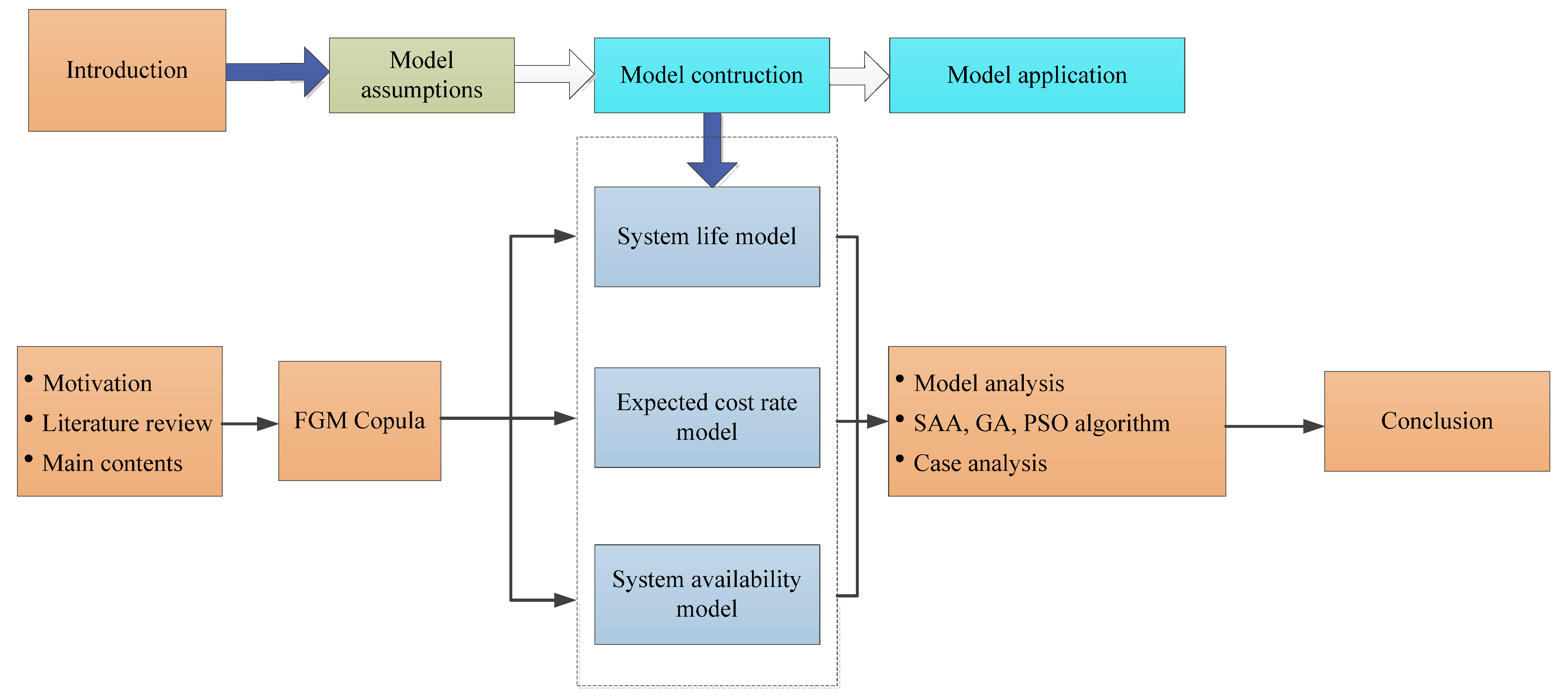
The rest of this paper is organized as follows. Section 2 introduces the general situation of the model and the basic assumptions followed by the establishment of the model, as well as provides the symbols in the model and their meanings. Section 3 shows the process of model establishment. Based on the copula function and taking the system life model as the starting point, the two-dimensional expected cost rate model and system availability model are established successively. The fourth section gives the basic steps of model solving. The fifth section is the case analysis, which mainly verifies the application of the model in the engine fuel fine filter, gives its optimal two-dimensional age replacement scheme, and puts forward reasonable suggestions for managers to make maintenance decisions combined with the results of the comparative analysis and sensitivity analysis. Some concluding remarks are presented in Section 6. The main structure of this paper is shown in Figure 1. The arrows represent the order in which relevant content appears in the paper.

2. Model Description, Assumptions and Notation

2.1. Model Description

The multi-component system is composed of several components in parallel. The two-dimensional age replacement strategy is adopted for the system, that is, the preventive replacement is carried out when the system runs to the specified two-dimensional preventive maintenance interval (T₀, U₀), where T₀ is the preventive maintenance interval in the time dimension, and the unit is year; U₀ is the preventive maintenance interval in the use degree dimension, and the unit is 10⁴ km. If the failure occurs between the two-dimensional age replacement intervals, the component shall be replaced, and the new age replacement period shall be recalculated again after the system is replaced.

2.2. Model Assumptions

(1)

The system consists of multiple components in parallel.

(2)

The multi-component system is not repairable, and the failure rate increases.

(3)

The utilization rate of the same user remains unchanged; the utilization rate of different users is a random variable and follows a certain distribution.

(4)

The failure response time is ignored, that is, it is replaced immediately after the failure.

(5)

The degradation of components and their corresponding degradation states are not explicitly considered (only their life and failure rate functions are used).

(6)

Maintenance activities are perfect (the replaced components are brand new) and independent of each other.

3. Model Construction

3.1. The System Life Model

A system is considered with n components. The components are connected in parallel. X_i is the life of the i-th component. It is a random variable subject to a certain distribution. Its probability density function, probability cumulative distribution function and failure rate function are: $f_i(\cdot )$, $F_i(\cdot )$ and ${\lambda }_i(\cdot )$, where $i=1,2,\dots ,n$.

The copula function is used to describe the parallel structure dependence between components, and its expression is [30]:

$$C(v_1,v_2,\dots ,v_n)=P(V_1\le v_1,V_2\le v_2,\dots ,V_n\le v_n)$$

(1)

The life of a parallel multi-component system under a certain utilization rate is expressed as $\chi (X_1,X_2,\dots ,X_N|r;\alpha )$, which is obviously a random variable. Its probability density function, probability cumulative distribution function and failure rate function are $f_{\chi }(\cdot |r;\alpha )$, $F_{\chi }(\cdot |r;\alpha )$ and ${\lambda }_{\chi }(\cdot |r;\alpha )$, respectively, and $\alpha$ is the component dependence parameter. For a parallel system, $\chi (X_1,X_2,\dots ,X_N|r;\alpha )=X_{N:N}$ means that the life of the parallel system is determined by the component with the longest life in the system. The parallel multi-component system is replaced at a certain time interval T_r or at time $\chi (X_1,X_2,\dots ,X_N|r;\alpha )$, depending on which event occurs first. Therefore, the actual life of a multi-component system can be expressed as:

$$X_{TRS}=\min [\chi (X_1,X_2,\dots ,X_N|r;\alpha ),T_r]$$

(2)

3.2. Two-Dimensional Age Replacement Expected Cost Rate Model

Since the specified two-dimensional age replacement interval is (T₀, U₀), the actual system age replacement interval T_r changes due to different utilization rates. Specifically:

$$T_r=\left\{\begin{array}{lll}{T}_0& & r\le U_0/T_0\\ U_0/r& & r>U_0/T_0\end{array}\right.$$

(3)

According to Equation (3), the usage is a linear function of time, and the coefficient of this function is the utilization rate, that is, $U=rT$. As shown in Figure 2a, when $r\le U_0/T_0$, because the utilization rate is a relatively low value, the system is replaced in the time dimension, that is, the replacement time interval $T_r=T_0$. As shown in Figure 2b, when $r>U_0/T_0$, because the utilization rate is a relatively high value, the system is replaced in the dimension of usage, that is, the replacement time interval $T_r=U_0/r$.

The reliability function of the multi-component system can be expressed as:

$$\begin{array}{ll}{\overline{F}}_{X_{TRS}}(t|r;\alpha )& =P(\min [\chi (X_1,X_2,\dots ,X_N|r;\alpha ),T_r]>t)\\ & =\underset{\chi (X_1,X_2,\dots ,X_N|r;\alpha )>t}{{\displaystyle \int \cdots }{\displaystyle \int }}dC[F_1(x_1|r),F_2(x_2|r),\dots ,F_N(x_N|r);\alpha ]\end{array}$$

(4)

Then, the average replacement time of the system can be expressed as:

$$E_{\alpha }(X_{TRS}|r)={\displaystyle \underset{0}{\overset{T_r}{\int }}\underset{\chi (X_1,X_2,\dots ,X_N|r;\alpha )>t}{{\displaystyle \int \cdots }{\displaystyle \int }}dC[F_1(x_1|r),F_2(x_2|r),\dots ,F_N(x_N|r);\alpha ]dt}$$

(5)

Then, the expected cost rate of the multi-component system in the replacement interval can be expressed as:

$$\begin{array}{ll}{C}_a(T_r;\alpha )& =\frac{C_f{F}_{\chi }(T_r|r;\alpha )+C_p\overline{F_{\chi }}(T_r|r;\alpha )}{E_{\alpha }(X_{TRS}|r)}\\ & =\frac{C_f+(C_p-C_f)\overline{F_{\chi }}(T_r|r;\alpha )}{E_{\alpha }(X_{TRS}|r)}\end{array}$$

(6)

The FGM copula function can adapt to the relatively weak correlation between marginal variables. Thus, the FGM copula function is considered to describe the dependence between components, which is in the form of:

$$C(v_1,v_2,\dots ,v_n;\alpha )={\displaystyle \prod _{j=1}^n{v}_j\{1+\alpha {\displaystyle \prod _{j=1}^n(1-v_j)}\}}$$

(7)

where $0<v_j<1,j=1,2,\dots ,n$ and $0<\alpha <1$. In particular, when $\alpha =0$, it indicates that there is no dependence between components.

Formulas (4) and (7) are combined to obtain:

$$\begin{array}{ll}{\overline{F}}_{X_{TRS}}(t|r;\alpha )& =1-C[F_1(t|r),F_2(t|r),\dots ,F_n(t|r);\alpha ]\\ & =1-M(t)-\alpha M(t)\overline{M}(t)\end{array}$$

(8)

where $M(t|r)={\displaystyle \prod _{j=1}^n{F}_j(t|r)}$, $\overline{M}(t|r)={\displaystyle \prod _{j=1}^n{\overline{F}}_j(t|r)}$.

Formulas (5) and (7) are combined to obtain average replacement time of the system:

$$E_{\alpha }(X_{TRS}|r)=T_r-{\displaystyle \underset{0}{\overset{T_r}{\int }}M(t)dt-\alpha {\displaystyle \underset{0}{\overset{T_r}{\int }}M(t)\overline{M}(t)}}dt$$

(9)

The expected cost rate of the multi-component system during the replacement interval is:

$$C_a(T_r;\alpha )=\frac{C_f+(C_p-C_f)[1-M(T_r)-\alpha M(T_r)\overline{M}(T_r)]}{T_r-{\displaystyle \underset{0}{\overset{T_r}{\int }}M(t)dt-\alpha {\displaystyle \underset{0}{\overset{T_r}{\int }}M(t)\overline{M}(t)}}dt}$$

(10)

Formulas (3) and (10) are combined, then the optimal $(T_0^{\ast },U_0^{\ast })$ is obtained and the minimization of $C_a(T_r;\alpha )$ is realized, and the $C_a(T_r;\alpha )$ is the optimal two-dimensional age replacement scheme. If $(T_0^{\ast },U_0^{\ast })$ does not exist, it is the best choice to replace it after failure.

3.3. Two-Dimensional Age Replacement Availability Model

MTTF is used to represent the expected duration of continuous operation of the system (the average time of operation of the system), and MTTR is used to represent the expected time required to replace the system; then, the availability of the system can be expressed as:

$$A=\frac{MTTF}{MTTF+MTTR}$$

(11)

The derivation method similar to the expected cost rate is used, the availability function of the system can be obtained as follows:

$$A(T_r;\alpha )=\frac{E_{\alpha }(X_{TRS}|r)}{E_{\alpha }(X_{TRS}|r)+T_f+(T_p-T_f)\overline{F_{\chi }}(T_r|r;\alpha )}$$

(12)

Formulas (3) and (12) are combined, then the optimal $(T_0^{\ast },U_0^{\ast })$ is obtained, and the maximization of $A(T_r;\alpha )$ is realized. If $(T_0^{\ast },U_0^{\ast })$ does not exist, it is the best choice to replace it after failure.

Then, MTTR and MTTF can be expressed as:

$$MTTR=T_f+(T_p-T_f)[1-M(t)-\alpha M(t)\overline{M}(t)]$$

(13)

$$MTTF=T_r-{\displaystyle \underset{0}{\overset{T_r}{\int }}M(t)dt-}\alpha {\displaystyle \underset{0}{\overset{T_r}{\int }}M(t)\overline{M}(t)dt}]$$

(14)

Formula (12) can be rewritten as:

$$A(T_r;\alpha )=\frac{T_r-{\displaystyle \underset{0}{\overset{T_r}{\int }}M(t)dt-\alpha {\displaystyle \underset{0}{\overset{T_r}{\int }}M(t)\overline{M}(t)}}dt}{T_r-{\displaystyle \underset{0}{\overset{T_r}{\int }}M(t)dt-\alpha {\displaystyle \underset{0}{\overset{T_r}{\int }}M(t)\overline{M}(t)}}dt+T_f+(T_p-T_f)[1-M(T_r)-\alpha M(T_r)\overline{M}(T_r)]}$$

(15)

4. Model Analysis

Due to the two-dimensional age replacement strategy, the time of replacement will change with the alteration of the utilization rate. The specific steps of solving the model are as follows:

Step 1: A group of (T₀, U₀) is given, and r₀ = U₀/T₀.

Step 2: When $r\le r_0$, $T_r=T_0$. In this case, the expected cost rate and expected availability are:

$$C_{\exp }(1)={\displaystyle \underset{r_l}{\overset{r_0}{\int }}{C}_a(T_0;\alpha )}dG(r)$$

(16)

$$A_{\exp }(1)={\displaystyle \underset{r_l}{\overset{r_0}{\int }}A(T_0;\alpha )}dG(r)$$

(17)

where $r_l$ is the lower limit of the utilization rate, and $G(r)$ is the probability cumulative distribution function to which the utilization rate obeys.

Step 3: $r_u$ is the upper limit of the utilization rate. $[r_0,r_u]$ is divided into k intervals on average, and each interval can be expressed as: $[r_{a-1},r_a),a=1,2,\dots ,k$. $r_a$ can be expressed as:

$$r_a=r_1+a\times \frac{r_u-r_1}{k},a=1,2,\dots ,k$$

(18)

Step 4: The method of transforming continuity into discreteness is adopted, and the average utilization rate of this interval is used to replace this interval for calculation. The average utilization rate of the interval can be expressed as:

$$\overline{r_a}={\displaystyle {\int }_{r_{a-1}}^{r_a}\frac{sg(s)}{G(r_a)-G(r_{a-1})}}ds$$

(19)

Step 5: The probability that the utilization rate falls in each interval is:

$$P_a=G(r_a)-G(r_{a-1})$$

(20)

Step 6: The expected cost rate and expected availability of each interval are calculated. The calculation formula is:

$$C_{\exp a}=C_a(U_0/\overline{r_a};\alpha )P_{a}a=1,2,\dots ,k$$

(21)

$$A_{\exp a}=A(U_0/\overline{r_a};\alpha )P_{a}a=1,2,\dots ,k$$

(22)

Step 7: When $r>r_0$, the expected cost rate and the expected availability are:

$$C_{\exp }(2)={\displaystyle \sum _{a=1}^k{C}_{\exp a}} a=1,2,\dots ,k$$

(23)

$$A_{\exp }(2)={\displaystyle \sum _{a=1}^k{A}_{\exp a}} a=1,2,\dots ,k$$

(24)

Step 8: Then, the total expected cost rate and total expected availability of the system during the two-dimensional age replacement interval are:

$$C_a=C_{\exp }(1)+C_{\exp }(2)$$

(25)

$$A=A_{\exp }(1)+A_{\exp }(2)$$

(26)

The specific process of solving the model is shown in Figure 3.

5. Case Analysis

5.1. Problem Description and Case Preparation

Taking the fuel fine filter of a certain type of engine as an example, the analysis is carried out. The fuel fine filter is used to filter out the fine impurities and moisture in diesel oil and provide clean diesel oil for the fuel injection pump and the injector to ensure its reliable operation. The fuel fine filter is composed of two filters in parallel.

The main failure mode of the fuel fine filter is that the fuel filter is blocked and dirty, resulting in insufficient fuel supply. Finally, the starting power is insufficient or even unable to start, resulting in vehicle paralysis. Therefore, the fuel fine filter should be replaced at regular intervals or after reaching a certain driving mileage. The purpose of this case is to determine the optimal two-dimensional age replacement interval of fuel fine filters, so as to minimize the expected cost rate or maximize the availability of fuel fine filters.

Based on the accelerated failure time (AFT) model, the failure rate function of the filter is constructed in this paper. Lawless [31] used the concept of accelerated failure time and proportional hazards models to construct the impact of utilization rate on system failure. This method has a certain theoretical basis and mature application.

Assuming that $T_s$ and $T_r$ represent the time of the first failure under the design utilization rate $r_s$ and utilization rate $r$, respectively, the relationship between them can be expressed as:

$$\frac{T_r}{T_s}={(\frac{r_s}{r})}^{\gamma }$$

(27)

$F_s(t;{\alpha }_s,\phi )$ is supposed as the cumulative failure distribution function under the design utilization rate $r_s$, where the scale parameters and shape parameters of the failure distribution under the design utilization rate are represented by ${\alpha }_s$ and $\phi$, respectively. When the utilization rate is $r$, the cumulative failure distribution function of the system has the same form as the cumulative failure distribution function of the system under the design utilization rate, but the scale parameter changes:

$${\alpha }_r={\alpha }_s{(\frac{r_s}{r})}^{\gamma }$$

(28)

where AFT parameter $\gamma \ge 1$. Based on this, when the utilization rate is $r$, the cumulative failure distribution function of the system can be expressed as:

$$F(t;{\alpha }_r,\phi )=F_s(t;{\alpha }_s{(\frac{r_s}{r})}^{\gamma },\phi )$$

(29)

The fuel fine filter is composed of two identical filters in parallel, and the utilization rate of the system follows a uniform distribution. Under the design utilization rate $r_s$, the cumulative failure distribution function of a single component is:

$$F_0(t;{\alpha }_s)=1-\exp [-{(t/{\alpha }_s)}^{\phi }]$$

(30)

Then, the cumulative failure distribution function of a single component is:

$$F(t|r)=F_s(t;{\alpha }_s{(\frac{r_s}{r})}^{\gamma },\phi )=1-\exp [-{(\frac{r}{r_s})}^{\gamma \phi }\frac{t^{\phi }}{{\alpha }_s^{\phi }}]$$

(31)

The fuel fine filter is mainly composed of two filters in parallel. According to Formula (13):

$$M(t|r)={\displaystyle \prod _{j=1}^2{F}_j(t|r)}={\{1-\exp [-{(\frac{r}{r_s})}^{\gamma \phi }\frac{t^{\phi }}{{\alpha }_s^{\phi }}]\}}^2$$

(32)

$$\overline{M}(t|r)={\displaystyle \prod _{j=1}^2{\overline{F}}_j(t|r)}=\{\exp [-2{(\frac{r}{r_s})}^{\gamma \phi }\frac{t^{\phi }}{{\alpha }_s^{\phi }}]\}$$

(33)

Other parameter settings of fuel fine filter are shown in

Table 1. Parameter setting.

Cp/CNY	Cf/CNY	Tp/Day	Tf/Day	${\mathit{r}}_{\mathit{s}}(\times 10 {\mathbf{km}}^4/\mathbf{Year})$	$\mathit{\gamma }$	$\mathit{\phi }$	${\mathit{\alpha }}_{\mathit{s}}$	${\mathit{r}}_{\mathit{l}} (\times 10 {\mathbf{km}}^4/\mathbf{Year})$	${\mathit{r}}_{\mathit{u}} (\times 10 {\mathbf{km}}^4/\mathbf{Year})$
5000	10,000	1	3	1	1.15	1.6	1.2	0.36	3.6

.

5.2. Optimal Two-Dimensional Age Replacement Scheme of the System

Using the parameter values set in Table 1 and based on the steps of solving the model in the model analysis, the change of the expected cost rate and availability of the system with the replacement interval is obtained, as shown in Figure 4 and Figure 5. In the figure, the unit of T₀ is a year, the unit of U₀ is 10⁴ km, and the unit of C is CNY. This rule also applies to all subsequent 3D images.

Figure 4 shows the change in the expected cost rate of the system with the alteration of the two-dimensional replacement interval. It can be seen from Figure 4 that the expected cost rate of the system is jointly affected by T₀ and U₀, and there is an optimal two-dimensional replacement interval (T₀, U₀) to minimize the expected cost rate of the system. Figure 5 shows the change in system availability with the alteration of a two-dimensional replacement interval. Similar to the expected cost rate, the system availability is affected by T₀ and U₀. There is an optimal two-dimensional replacement interval (T₀, U₀), so that the system has the highest availability during the replacement interval.

It can be seen from Figure 4 and Figure 5 that T₀ has little impact on the system warranty cost and availability, that is, when U₀ is fixed, the change in the time interval for replacing the system will not cause a significant change in the system warranty cost and availability. The main failure mode of the fuel fine filter is that the fuel filter is blocked and dirty, resulting in efficient fuel supply. Therefore, the mileage has a great impact on the failure of the fuel fine filter, and the two have a strong correlation. Furthermore, as time goes by, the components that make up the fuel fine filter may corrode, but this process is very slow. Therefore, calendar time is not the main factor that causes the failure of the fuel fine filter. Thus, there is weak dependency between T₀ and system availability/warranty cost. This is also the reason why this paper chooses to use the AFT model to construct the failure rate function.

In order to find the optimal two-dimensional replacement interval of the system, taking the minimum expected cost rate and the highest availability as the decision objectives, the optimal two-dimensional age replacement scheme is solved based on the intelligent optimization algorithm. The particle swarm optimization (PSO) algorithm [32], genetic algorithm (GA) [33] and simulated annealing algorithm (SAA) [34] are compared and analyzed. The iteration number is 700, and the population number is 100 (this parameter is not involved in the SAA). The replication strategy of GA is the elite selection method, with a proportion of 10, a crossover probability of 0.8, and a mutation probability of 0.01. The SAA is set to iterate 500 times per temperature, and the initial temperature is 10,000. The cooling rate is 0.9. The inertia weight of the PSO algorithm is 0.9, the self-adjustment weight is 1.49, and the social-adjustment weight is 1.49. The value range of U₀ is (0 km, 10 × 10⁴ km), and the value range of T₀ is (0 years, 5 years). The initial value of the two-dimensional age replacement interval (T₀, U₀) is set as (2 years, 5 × 10⁴ km). Aiming at the lowest warranty cost rate, the iterative process of each algorithm is shown in Figure 6.

Figure 6a–c show the convergence curves of the PSO algorithm, SAA and GA, respectively, when aiming at the lowest warranty cost rate. Aiming at the maximum availability, the iterative process of each algorithm is shown in Figure 7.

Figure 7a–c show the convergence curves of the PSO algorithm, SAA and GA, respectively, when aiming at the maximum availability. The results of each algorithm under different decision objectives are shown in

Table 2. The results of each algorithm.

Algorithm	Warranty Cost Rate (CNY)	Availability
PSO	66,245.7	0.66453
GA	63,598.6	0.68352
SAA	62,945.1	0.71265

.

The above three algorithms are global optimization algorithms, which can obtain the best possible global optimal solution region in the sense of probability through probability search. Therefore, the results of each run may be different. In order to test the stability of the results, the three algorithms are run 100 times with the same parameters, and the average value of the results of 100 runs is calculated for comparison. The optimal value obtained after each run of the program is shown in Figure 8. The average value of 100 operations is shown in

Table 3. The results and operation time of each algorithm.

Algorithm	Average Cost (CNY)	Average Availability
PSO	66,276.4	0.665
GA	63,582.3	0.682
SAA	62,941.6	0.713

.

Through comparison, it can be found that SAA can obtain a lower warranty cost rate and higher availability, and can converge earlier with higher operational efficiency; thus, it has more advantages in solving this model. The schematic diagram of the optimization process for the SAA is shown in Figure 9.

In Figure 9, the black marked points show the iterative process of the simulated annealing algorithm. Figure 9a shows that with the minimum expected cost rate as the goal, the optimal two-dimensional age replacement scheme is (2.2 years, 9000 km), and the expected cost rate is 62,945.1 CNY/year. Figure 9b shows that taking the maximum system availability as the goal, the optimal two-dimensional age replacement scheme is (1.8 years, 6000 km), and the availability is 0.71265. It can be seen that the model established in this paper can provide technical support for determining the optimal age replacement scheme under different decision objectives.

Table 4. Expected cost rate under different two-dimensional age replacement schemes.

T0/Years	U0/104 km
	0.1	0.3	1	3	5	6	7	8	9	10
1	251,312	92,389.5	63,218.9	65,378.5	65,379.4	65,379.6	65,380.1	65,381.2	65,383.3	65,386.4
2	251,316	92,389.9	63,217.6	65,377.3	65,378.3	65,378.5	65,379.3	65,380.3	65,382.3	65,384.3
3	251,327	92,390.3	63,217.9	65,377.9	65,378.7	65,378.8	65,379.9	65,381.1	65,382	65,386
4	251,334	92,394	63,218.2	65,379	65,382	65,383	65,383.7	65,386	65,395	65,399
5	251,403	92,401.5	63,227.2	65,386	65,394	65,396	65,398	65,402	65,452	65,503

and

Table 5. Availability under different two-dimensional age replacement schemes.

T0/Years	U0/104 km
	0.1	0.3	1	3	5	6	7	8	9	10
1	0.477	0.675	0.698	0.682	0.682	0.682	0.682	0.682	0.682	0.682
2	0.477	0.675	0.698	0.682	0.682	0.682	0.682	0.682	0.682	0.682
3	0.477	0.675	0.698	0.682	0.682	0.682	0.682	0.682	0.682	0.682
4	0.477	0.675	0.698	0.682	0.682	0.682	0.682	0.682	0.682	0.682
5	0.477	0.675	0.698	0.681	0.682	0.682	0.682	0.682	0.682	0.682

show the expected cost rate and availability of the system under more two-dimensional age replacement schemes.

It can be seen from Table 4 and Table 5 that the model proposed in this paper can provide a scientific basis for cost calculation and availability estimation under the two-dimensional age replacement strategy of the system.

5.3. Comparative Analysis

5.3.1. Comparison between Weibull Distribution and Normal Distribution

In the analysis of 5.2, the utilization rate obeys uniform distribution, but in reality, the distribution of the utilization rate is not always uniform. To determine the utilization rate distribution, it is necessary to use a specific distribution to fit the parameters on the basis of sufficient utilization rate data. There are many methods of parameter fitting, and the most commonly used is maximum likelihood estimation. This method is relatively simple and easy to implement. In the field of two-dimensional warranty research, uniform distribution, normal distribution and Weibull distribution are the most common distribution forms of utilization rate r. To facilitate comparison, it is assumed that the three distribution forms of utilization have the same upper and lower limits, and the maximum utilization rate is 3.6 × 10⁴ km/year, while the minimum utilization rate is 0.36 × 10⁴ km/year. Moreover, it is assumed that the mean value of normal distribution is 2 × 10⁴ km/year, and the standard deviation is 0.8. Since the value range of the normal distribution variable is (−∞, +∞), but the utilization rate cannot be negative, this paper makes an approximate estimation of the parameters of the normal distribution to ensure that the integral value within the utilization rate interval (0.36, 3.6) is greater than 0.95. In order to verify the influence of different utilization rate distributions on the optimal two-dimensional age replacement scheme, the optimal two-dimensional age replacement scheme of the system under the condition that the utilization rate obeys the two-parameter Weibull distribution, normal distribution and uniform distribution is compared. Both normal distribution and Weibull distribution are commonly used. It is known that the utilization rate follows the two-parameter Weibull distribution, the scale parameter m = 20,000 km/year, and the shape parameter n = 2.5. The probability density function of this distribution is:

$$g(r)=\frac{n}{m}{(\frac{r}{m})}^{n-1}{e}^{-{(\frac{r}{m})}^n}(0.36<r<3.6)$$

(34)

The other distribution is normal distribution, with mean value $\mu =2\times {10}^4\mathrm{km}/\mathrm{year}$ and standard deviation $\sigma =0.8\times {10}^4\mathrm{km}/\mathrm{year}$. The probability density function of this distribution is:

$$g(r,\mu ,\sigma )=\frac{1}{\sigma \sqrt{2\pi }}{e}^{-\frac{{(r-\mu )}^2}{2{\sigma }^2}}(0.36<r<3.6)$$

(35)

The curve corresponding to the probability density function is shown in Figure 10.

Figure 10a shows the probability density function image when the utilization follows a Weibull distribution, and Figure 10b shows the probability density function image when the utilization follows a normal distribution. Based on the simulated annealing algorithm, the iterative schematic diagrams of the expected cost rate and availability of the system when the utilization is subject to two-parameter Weibull distribution and normal distribution are obtained by using the same steps as when the utilization is subject to uniform distribution in 5.2, as shown in Figure 11 and Figure 12.

Figure 11 shows the iterative diagram of the expected cost rate and availability of the system when the utilization rate follows the two-parameter Weibull distribution. It can be seen from Figure 11a that when the utilization rate obeys the two-parameter Weibull distribution, the optimal two-dimensional age replacement scheme of the system is (2.5 years, 8000 km), and the expected cost rate is 71,263.3 CNY/year. It can be seen from Figure 11b that the optimal two-dimensional age replacement scheme is (2 years, 9000 km), and the availability is 0.687. The availability is a little low. This is mainly due to the high failure rate of the fuel fine filter in this case. Because of the high failure rate of the fuel fine filter, within a preventive replacement interval, the fuel fine filter needs to be replaced after multiple failures, which not only increases the warranty cost, but also reduces the availability. In addition, this model also considers the failure interaction between components and introduces parameter α to describe the correlation of failure time between components, which further increases the failure rate of the fuel fine filter and reduces the availability. A value of 0.687 is the availability corresponding to the optimal two-dimensional replacement scheme found when the utilization rate follows the two-parameter Weibull distribution. This value is less than the availability corresponding to the optimal two-dimensional age replacement scheme found when the utilization rate follows the uniform distribution and normal distribution. This is mainly because when the utilization rate follows the two-parameter Weibull distribution, the higher utilization rate appears with a higher probability; thus, the failure of the fuel fine filter is more frequent. This factor can also lead to reduced availability. Figure 12 shows the iterative diagram of the expected cost rate and availability of the system when the utilization is normally distributed. It can be seen from Figure 12a that taking the lowest expected cost rate as the goal, the optimal two-dimensional age replacement scheme of the system is (1.9 years, 11,000 km). At this time, the expected cost rate is 46,213.1 CNY/year. It can be seen from Figure 12b that taking the maximum system availability as the goal, the optimal two-dimensional age replacement scheme is (3.1 years, 13,000 km), and the availability is 0.762. When the utilization rate follows different distributions, the comparison of the optimal two-dimensional age replacement schemes of the system under different decision objectives is shown in

Table 6. The optimal scheme when the utilization rate follows different distributions.

Distribution Type	The Lowest Expected Cost Rate as the Goal		Optimal Value (CNY)	The Highest Availability as the Goal		Optimal Value
	T0 (Years)	U0 (104 km)		T0 (Years)	U0 (104 km)
Uniform distribution	2.2	0.9	62,945.1	1.8	0.6	0.7127
Two-parameter Weibull distribution	2.5	0.8	71,263.3	2	0.9	0.687
Normal distribution	1.9	1.1	46,213.1	3.1	1.3	0.762

.

It can be seen from Table 6 that the two-dimensional age replacement scheme and optimal value of the system are quite different under different utilization rate distributions. Therefore, before formulating the warranty scheme of the system, the manufacturer should conduct sufficient market research to clarify the utilization rate of potential consumers as much as possible and then use the model and method proposed in this paper to formulate a more accurate two-dimensional age replacement scheme of the system, which is beneficial to the manufacturer to save the warranty cost and improve the availability of the system.

5.3.2. Comparison between One-Dimensional Age Replacement and Two-Dimensional Age Replacement

The maintenance strategy adopted in this paper is the two-dimensional age replacement strategy, that is, the system is replaced in the warranty period considering both the time dimension and the mileage dimension. The commonly used age replacement strategy is a one-dimensional age replacement strategy at present, that is, the system is replaced only considering the calendar time during the warranty period. In order to reflect the advantages of two-dimensional age replacement, the two strategies are compared.

In the study above, the scheme of two-dimensional age replacement has been obtained by SAA. The situation of one-dimensional age replacement is analyzed below. U₀ is taken as its maximum value of 100,000 km, and it can be obtained by using the same calculation method as 5.2 that when the age replacement interval is 1.8 years, the minimum warranty cost rate is 63,785.6 CNY. When the age replacement interval is 1.3 years, the highest availability is 0.6914. It can be seen that the two-dimensional age replacement strategy has more advantages in reducing warranty costs and improving availability compared with the one-dimensional age replacement strategy.

5.4. Sensitivity Analysis

$\alpha$ is the parameter of the copula function, which measures the correlation strength between variables. In the case study, $\alpha$ indicates the correlation between the failure times of the two filter bodies of the fuel fine filter; thus, it represents the physical quantity of failure interaction between components. The correlation coefficient can be determined by the following methods:

(1)

Obtained by probability theory;

(2)

Based on experience of designers, manufacturers and maintenance personnel;

(3)

Based on mechanical or dynamic estimation;

(4)

Based on laboratory experiments.

In order to explore the influence of different values of $\alpha$ on the optimal age replacement scheme of the system, the value of $\alpha$ is transformed to obtain the optimal age replacement scheme of the system under different values of $\alpha$, as shown in

Table 7. The optimal scheme under different.

$\mathit{\alpha }$	The Lowest Expected Cost Rate as the Goal		Optimal Value (CNY)	The Highest Availability as the Goal		Optimal Value
	T0 (Years)	U0 (104 km)		T0 (Years)	U0 (104 km)
0	1.8	0.7	58,412.3	1.9	0.8	0.7245
0.5	2.2	0.9	62,945.1	1.8	0.6	0.7127
1	2.4	1.2	68,521.4	1.5	0.4	0.6512

.

Figure 13a,b show the lowest expected cost rate and highest availability of the system under different $\alpha$ values, respectively. It can be seen from Table 6 and Figure 13 that with the increase in $\alpha$, the optimal two-dimensional age replacement scheme of the system will change greatly, and the warranty cost and system availability corresponding to the optimal scheme will change tremendously. Specifically, with the increase in $\alpha$, that is, the correlation of failure time between components becomes stronger and stronger, the failure of one component has a greater and greater impact on another component, the warranty cost of the system during the warranty period will increase, and the availability will decrease. This shows that in the product design and manufacturing stage, the transmission of failure between components should be prevented, and the value of $\alpha$ can be reduced as much as possible by increasing the flexible connection between components.

6. Conclusions

This paper mainly studies the two-dimensional age replacement strategy of a parallel system with structural dependence. The FGM copula function is used to describe the dependence between multi-components, and a two-dimensional age replacement strategy optimization method based on the minimum expected cost rate function and maximum availability function is proposed. The intelligent optimization algorithm is used to find the optimal decision-making scheme. Finally, the application of the model in an engine fuel fine filter is discussed. Through an optimization solution, comparative analysis and sensitivity analysis, the following conclusions can be obtained.

1. The model proposed in this paper can provide an optimal two-dimensional age replacement scheme for a parallel system with structural dependence and provide a scientific basis for the maintenance cost calculation and availability estimation of the system. When solving such problems, compared with the PSO algorithm and GA, SAA can obtain a lower warranty cost rate and higher availability with higher operational efficiency.

2. The utilization rate of the system has a great impact on the optimal two-dimensional age replacement scheme. Therefore, this paper suggests that manufacturers should conduct sufficient market research before formulating the warranty scheme of the system, clarify the utilization rate of potential consumers as much as possible, and then use the models and methods proposed in this paper to formulate a more accurate two-dimensional age replacement scheme of the system, so as to save maintenance costs and improve system availability. In addition, manufacturers can save warranty costs and improve system availability by providing a two-dimensional age replacement strategy.

3. As the correlation coefficient $\alpha$ between components increases, the system maintenance cost increases, and the availability decreases. This shows that in the product design and manufacturing stage, the transmission of failure between components should be prevented by increasing the flexible connection between components, so as to reduce the correlation between components.

This single example can represent more general application scenarios. The application of this model requires two conditions: one is that the warranty object is a multi-component parallel system, and the other is that there is a correlation between the failure times of components, such as the Warm Standby Redundant. On the basis of meeting these two conditions, by fitting the failure rate function and utilization rate function as well as estimating the value of α, this model can be used to obtain the two-dimensional age replacement plan under different decision-making objectives. Some extensions of the proposed model in this paper can be considered for future study:

• The parallel system is extended to series systems, hybrid systems, cold reserve systems and other types of systems to improve the applicability of the model.
• There are many kinds of copula functions. We can explore the method to determine the optimal copula function. The applicability of the copula function is worth studying.
• The maintenance strategy mainly adopted in this paper is age replacement. In addition to age replacement, block replacement, failure detection and function inspection are common preventive maintenance methods. Future research can focus on maintenance decisions under different preventive maintenance methods.
• In the next step of research, we can consider taking the lowest warranty cost and the highest availability as the decision objectives, using the NSGA algorithm to solve the optimal warranty scheme, taking into account the interests of both manufacturers and users, and expanding the application scope of the model.

References

1. Wang, J.; Miao, Y.; Yi, Y.; Huang, D. An imperfect age-based and condition-based opportunistic maintenance model for a two-unit series system. Comput. Ind. Eng. 2021, 160, 107583. [Google Scholar] [CrossRef]
2. Gan, S.; Song, Z.; Zhang, L. A maintenance strategy based on system reliability considering imperfect corrective maintenance and shocks. Comput. Ind. Eng. 2022, 164, 107886. [Google Scholar] [CrossRef]
3. Assis, R.; Marques, P.C. A dynamic methodology for setting up inspection time intervals in conditional preventive maintenance. Appl. Sci. 2021, 11, 8715. [Google Scholar] [CrossRef]
4. Barlow, R.E.; Proschan, F. Mathematical Theory of Reliability; John Wiley and Sons: Hoboken, NJ, USA, 1965. [Google Scholar]
5. Sheu, S.H.; Chang, C.C. An extended periodic imperfect preventive maintenance model with age-dependent failure type. IEEE Trans. Reliab. 2009, 58, 397–405. [Google Scholar] [CrossRef]
6. Sheu, S.-H.; Zhang, Z.G. An optimal age replacement policy for Multi-State Systems. IEEE Trans. Reliab. 2013, 62, 722–735. [Google Scholar] [CrossRef]
7. Dagpunar, J.S. Some necessary and sufficient conditions for age replacement with non-zero downtimes. J. Oper. Res. Soc. 1994, 45, 225–229. [Google Scholar] [CrossRef]
8. Jiang, R.; Ji, P. Age replacement policy: A multi-attribute Value Model. Reliab. Eng. Syst. Saf. 2002, 76, 311–318. [Google Scholar] [CrossRef]
9. Safaei, F.; Ahmadi, J.; Sadeghpour Gildeh, B. An optimal planned replacement time based on availability and cost functions for a system subject to three types of failures. Comput. Ind. Eng. 2018, 124, 77–87. [Google Scholar] [CrossRef]
10. Finkelstein, M.; Cha, J.H.; Levitin, G. On a new age-replacement policy for items with observed stochastic degradation. Qual. Reliab. Eng. Int. 2020, 36, 1132–1143. [Google Scholar] [CrossRef]
11. Huang, Y.-S.; Huang, C.-D.; Ho, J.-W. A customized two-dimensional extended warranty with preventive maintenance. Eur. J. Oper. Res. 2017, 257, 971–978. [Google Scholar] [CrossRef]
12. Shahanaghi, K.; Noorossana, R.; Jalali-Naini, S.G.; Heydari, M. Failure modeling and optimizing preventive maintenance strategy during two-dimensional extended warranty contracts. Eng. Fail. Anal. 2013, 28, 90–102. [Google Scholar] [CrossRef]
13. Varnosafaderani, S.; Chukova, S. A two-dimensional warranty servicing strategy based on reduction in product failure intensity. Comput. Math. Appl. 2012, 63, 201–213. [Google Scholar] [CrossRef] [Green Version]
14. Bouguerra, S.; Rezg, N.; Chelbi, A. A decision model for adopting an extended two-dimensional warranty considering different maintenance policies with variable customer’s behavior. IFAC Proc. Vol. 2012, 45, 968–974. [Google Scholar] [CrossRef]
15. Mitra, A. Warranty parameters for extended two-dimensional warranties incorporating consumer preferences. Eur. J. Oper. Res. 2021, 291, 525–535. [Google Scholar] [CrossRef]
16. Taleizadeh, A.A.; Mokhtarzadeh, M. Pricing and two-dimensional warranty policy of multi-products with online and offline channels using a value-at-risk approach. Comput. Ind. Eng. 2020, 148, 106674. [Google Scholar] [CrossRef]
17. Cheng, Z.H.; Wang, Q.; Bai, Y.S.; Zhao, R.D.; Guo, S.K. Availability optimization model of two-dimensional warranty equipment. J. Acad. Armored Force Eng. 2019, 33, 34–39. [Google Scholar]
18. Cheng, Z.H.; Yang, Z.Y.; Zhao, Z.; Wang, Y.B.; Li, Z.W. Preventive maintenance strategy optimizing model under two-dimensional warranty policy. Eksploat. I Niezawodn.—Maint. Reliab. 2015, 17, 365–372. [Google Scholar] [CrossRef]
19. Wang, L.; Pei, Z.; Zhu, H.; Liu, B. Optimising extended warranty policies following the two-dimensional warranty with repair time threshold. Eksploat. I Niezawodn.—Maint. Reliab. 2018, 20, 523–530. [Google Scholar] [CrossRef]
20. Husniah, H.; Iskandar, B.P. Modelling two-dimensional lease contract with preventive maintenance and servicing strategy. J. Teknol. 2016, 78, 19–25. [Google Scholar] [CrossRef] [Green Version]
21. Dekker, R.; Wildeman, R.E.; van der Duyn Schouten, F.A. A review of multi-component maintenance models with economic dependence. Math. Methods Oper. Res. 1997, 45, 411–435. [Google Scholar] [CrossRef] [Green Version]
22. Nicolai, R.P.; Dekker, R. Optimal Maintenance of multi-component systems: A Review. Springer Ser. Reliab. Eng. 2000, 263–286. [Google Scholar] [CrossRef]
23. Thomas, L.C. A survey of maintenance and replacement models for maintainability and reliability of multi-item systems. Reliab. Eng. 1986, 16, 297–309. [Google Scholar] [CrossRef]
24. Sklar, A. Fonctions de repartition an dimensions et leurs marges. Publ. Inst. Stat. Univ. Paris 1959, 8, 229–231. [Google Scholar]
25. Tang, X.-S.; Li, D.-Q.; Zhou, C.-B.; Phoon, K.-K.; Zhang, L.-M. Impact of copulas for Modeling Bivariate Distributions on System Reliability. Struct. Saf. 2013, 44, 80–90. [Google Scholar] [CrossRef]
26. Xie, K.; Li, Y.; Li, W. Modelling wind speed dependence in system reliability assessment using copulas. IET Renew. Power Gener. 2012, 6, 392–399. [Google Scholar] [CrossRef]
27. Yang, S.C.; Liu, T.J.; Hong, H.P. Reliability of Tower and tower-line systems under spatiotemporally varying wind or earthquake loads. J. Struct. Eng. 2017, 143, 04017137. [Google Scholar] [CrossRef]
28. Guo, C.; Wang, W.; Guo, B.; Peng, R. Maintenance optimization for systems with dependent competing risks using a copula function. Eksploat. I Niezawodn.-Maint. Reliab. 2013, 15, 9–17. [Google Scholar]
29. Li, H.; Deloux, E.; Dieulle, L. A condition-based maintenance policy for multi-component systems with Lévy copulas dependence. Reliab. Eng. Syst. Saf. 2016, 149, 44–55. [Google Scholar] [CrossRef]
30. Liu, Y.; Chen, Y. Dynamic Reliability Evaluation of High-Speed Train Gearbox Based on Copula Function. IEEE Access 2022, 10, 51792–51803. [Google Scholar] [CrossRef]
31. Lawless, J.; Hu, J.; Cao, J. Methods for the estimation of failure distributions and rates from automobile warranty data. Lifetime Data Anal. 1995, 1, 227–240. [Google Scholar] [CrossRef]
32. Lin, D.P.; Jin, B.P.; Chang, D.F. A PSO approach for the integrated maintenance model. Reliab. Eng. Syst. Saf. 2020, 193, 106625. [Google Scholar] [CrossRef]
33. Yu, A.J.; Seif, J. Minimizing tardiness and maintenance costs in flow shop scheduling by a lower-bound-based GA. Comput. Ind. Eng. 2016, 97, 26–40. [Google Scholar] [CrossRef]
34. He, F.; Ye, Q. A bearing fault diagnosis method based on wavelet packet transform and convolutional neural network optimized by simulated annealing algorithm. Sensors 2022, 22, 1410. [Google Scholar] [CrossRef]
Figure 1. Thesis structure.
Processes 10 02519 g001
Figure 2. The real replacement time of a system. (a) r U 0 / T 0 , (b) r > U 0 / T 0 . Red line: Nominal utilization rate; Blue line: Actual utilization rate.
Processes 10 02519 g002
Figure 3. Model solving process.
Processes 10 02519 g003
Figure 4. System expected cost rate change.
Processes 10 02519 g004
Figure 5. System availability change.
Processes 10 02519 g005
Figure 6. The iterative process of each algorithm when aiming at the lowest warranty cost rate. (a) Convergence curve of PSO algorithm, (b) convergence curve of SAA, (c) convergence curve of GA.
Processes 10 02519 g006
Figure 7. The iterative process of each algorithm when aiming at the maximum availability. (a) Convergence curve of PSO algorithm, (b) convergence curve of SAA, (c) convergence curve of GA.
Processes 10 02519 g007
Figure 8. Optimal value of each algorithm run. (a) Changes in availability, (b) Changes in warranty cost.
Processes 10 02519 g008
Figure 9. Algorithm iteration diagram. (a) Changes in warranty cost, (b) Changes in availability.
Processes 10 02519 g009
Figure 10. Probability density function of different utilization rates: (a) Weibull distribution, (b) normal distribution.
Processes 10 02519 g010
Figure 11. Iteration when utilization rate follows Weibull distribution. (a) Minimum warranty cost under Weibull distribution, (b) The highest availability under Weibull distribution.
Processes 10 02519 g011
Figure 12. Iteration when utilization rate follows normal distribution. (a) Minimum warranty cost under normal distribution, (b) The highest availability under normal distribution.
Processes 10 02519 g012
Figure 13. Sensitivity analysis of α . (a) Minimum warranty cost under different α , (b) The highest availability under different α .
Processes 10 02519 g013