Deep Hierarchical Interval Type 2 Self-Organizing Fuzzy System for Data-Driven Robot Control

Abstract

To solve the dimensional explosion problem, this paper proposes a new architecture for the fuzzy system, the deep hierarchical self-organizing interval type-2 fuzzy system (DHSOIT2FS). Each sub-fuzzy system is a self-organizing interval type-2 fuzzy system, constructed online, with rules constructed by a rule online update algorithm, consequent parameters updated by iterative least squares, and antecedent parameters are updated using a gradient descent algorithm. DHSOIT2FS uses a classic serial-layered structure to build the overall framework. The first layer uses the first two dimensions of data as input. Each subsequent layer uses the output of the previous layer with the next dimensional data as input until it is built. During the training process, each data point is trained with DHSOIT2FS before passing in the next data point to achieve online construction. The effectiveness of the approach in this paper is illustrated using two numerical simulation examples. The proposed method is also applied to a data-driven control example of a single-link robot and achieves good tracking results.

1. Introduction

High latitude, in addition to a large order of magnitude data from data streams, is becoming the most common data type in many real-world applications [1]. Datastream data are quick and prone to conceptual drift. Therefore, it has become a popular problem for research in recent years [2]. Self-organizing fuzzy systems are effective structures for confronting this problem. Self-organizing fuzzy systems are powerful tools that are widely used for real-time non-stationary problem approximation. There are many developments in recent years [3,4,5]. Online self-organizing fuzzy systems can handle streaming data. After each datum comes in, the self-organizing fuzzy system only needs to adjust a few parameters instead of adjusting all parameters.

Fuzzy logic systems (FLSs) have been successfully used in a variety of areas [6,7,8,9]. However, most of these studies focus on type 1 FLSs. In recent years, studies on interval type 2 (IT2) FLSs have drawn much attention [10,11,12], and a complete theory of IT2 FLSs has been developed in [13]. IT2 FLSs are extensions of type 1 FLSs, where the membership value of an IT2 fuzzy set is a type 1 fuzzy number. IT2 FLSs appear to be a more promising method than their type 1 counterparts in handling problems with uncertainties such as noisy data and different word meanings. IT2 fuzzy sets allow researchers to model and minimize the effects of uncertainties in rule-based systems. Successful applications of IT2 FLSs include areas of signal processing [10,11], control [13,14,15], and medical applications [16].

Hierarchical fuzzy systems can be used to solve the problem of rule explosion. Each sub-fuzzy system is connected in a layer-to-layer fashion [17,18]. There are many ways to connect hierarchical fuzzy systems. The most classical ones are serial and stacked connections. Using serial connections can effectively reduce the number of rules. Hierarchical fuzzy systems also have practical applications in many ways [19,20].

The great success of deep convolutional neural networks (DCNN) [21] in solving complex practical problems [22,23,24] reveals a basic fact that multilevel structures are very powerful models in representing complex relationships. The main problems of DCNN are the substantial computational load required to train the many parameters of the DCNN and the lack of interpretability for the large number of model parameters [25]. To solve this problem, some scholars try to combine fuzzy systems with deep learning to obtain deep fuzzy neural networks. Currently, there is also substantial literature combining deep learning with fuzzy systems [26,27,28]. It can appropriately improve the interpretability of the system and reduce the computation time.

In this paper, we mainly combine the self-organizing interval type 2 fuzzy system with the deep hierarchical fuzzy system to form the deep hierarchical self-organizing interval type 2 fuzzy system (DHSOIT2FS). Each sub-fuzzy system is generated by self-organized construction. The structure of the sub-fuzzy system is formed by the self-organization of online data flow. Then, antecedent and consequent parameters are adjusted by gradient descent and iterative least squares algorithms. A serial hierarchical architecture is also used to combine multiple sub-fuzzy systems to form the DHSOIT2FS. When training the entire system, each data point is trained in turn for each sub-fuzzy system until all sub-fuzzy systems are trained. The effectiveness of the proposed algorithm is then illustrated in two numerical simulation examples and an actual single-link robot control simulation example.

The rest of this paper is organized as follows. Section 2 introduces the interval type 2 fuzzy system. Section 3 describes the construction method of DHSOIT2FS. Section 4 shows two numerical simulation examples and a data-driven robot control example. Finally, the conclusion is presented in Section 5.

2. Interval Type-2 Fuzzy System

In this section, we introduce information on interval type 2 fuzzy systems.

The IT2 FLS uses first-order TSK-type rules, and each rule has the following form:

$$\begin{array}{ll}\mathrm{Rule}i:& \mathrm{If}{x}_1\left(k\right)\mathrm{is}{A}_1^i,\dots ,\mathrm{and}{x}_n\left(k\right)\mathrm{is}{A}_n^i\\ & \mathrm{Then}y\mathrm{is}{\tilde{a}}_0^i+\sum _{j=1}^n{\tilde{a}}_j^i{x}_j\left(k\right),i=1,\dots ,R\end{array}$$

(1)

where $x_j\left(k\right),j=1\dots n$ is the input variable, and antecedent fuzzy set $A_j^i,i=1\dots R$, $j=1\dots n$ is an IT2 fuzzy set. k represents the sampling serial number. y is the output variable, and R is the number of rules. Consequent parameters ${\tilde{a}}_j^i,i=1\dots R,j=0\dots n$ are interval sets:

$$\begin{array}{l}{\tilde{a}}_j^i=\left[c_j^i-d_j^i,c_j^i+d_j^i\right],j=0,\dots ,n\end{array}$$

(2)

where $c_j^i$ and $d_j^i$ represent the central value and range of ${\tilde{a}}_j^i$, respectively. The IT2 FLS consists of a fuzzifier, inference engine, type reducer, and defuzzifier.

The fuzzier maps a crisp value to an IT2 fuzzy set. A Gaussian membership function with an uncertain mean, m, and a fixed standard deviation, $\sigma$, is used in this paper, which is described by the following:

$$\begin{array}{ll}{\mu }_j^i\left(x_{{}_j}\right)& =exp\left\{{\left(\frac{x_j-m_j^i}{{\sigma }_j^i}\right)}^2\right\}\\ & \equiv N\left(m_j^i,{\sigma }_j^i;x_{{}_j}\right),m_j^i\in \left[m_{j1}^i,m_{j2}^i\right]\end{array}$$

(3)

where $m_{j1}^i,m_{j2}^i$ represent the left mean and right mean of the Gaussian membership function, respectively. The membership degree ${\mu }_j^i\left(x_{{}_j}\right)$ is denoted by ${\mu }_j^i\left(x_{{}_j}\right)=\left[{\overline{\mu }}_j^i\left(x_j\right),{\underline{\mu }}_j^i\left(x_j\right)\right]$. ${\overline{\mu }}_j^i\left(x_j\right)$ and ${\underline{\mu }}_j^i\left(x_j\right)$ denote the upper membership degree and lower membership degree, respectively, which are calculated as follows.

$${\overline{\mu }}_j^i\left(x_j\right)=\left\{\begin{array}{cc}N\left(m_{j1}^i,{\sigma }_j^i;x_j\right)& x_j<m_{j1}^i\\ 1& m_{j1}^i\le x_j\le m_{j2}^i\\ N\left(m_{j2}^i,{\sigma }_j^i;x_j\right)& x_j>m_{j2}^i\end{array}\right.$$

(4)

$${\underline{\mu }}_j^i\left(x_j\right)=\left\{\begin{array}{cc}N\left(m_{j2}^i,{\sigma }_j^i;x_j\right)& x_j\le \left(m_{j1}^i+m_{j2}^i\right)/2\\ N\left(m_{j1}^i,{\sigma }_j^i;x_j\right)& x_j>\left(m_{j1}^i+m_{j2}^i\right)/2\end{array}\right.$$

(5)

The fire strength of the ith rule is given as follows:

$$f_i=\left[\begin{array}{cc}{\prod }_{j=1}^n{\underline{\mu }}_j^i\left(x_j\right)& {\prod }_{j=1}^n{\overline{\mu }}_j^i\left(x_j\right)\end{array}\right]=\left[\begin{array}{cc}{\underline{f}}_i& {\overline{f}}_i\end{array}\right]$$

(6)

where $f_i$ denotes the fire strength interval of the $i_{th}$ rule; ${\underline{f}}_i$ and ${\overline{f}}_i$ represent the lower and upper bounds of the activation intensity, respectively. Let $x_0\triangleq 1$; the output of each rule is an interval vaule denoted by $[g_i^l,g_i^r]$.

$$\begin{array}{c}\left[g_i^l,g_i^r\right]=\left[\sum _{j=0}^n{c}_j^i{x}_j-\sum _{j=0}^n\left|x_j\right|s_j^i,\sum _{j=0}^n{c}_j^i{x}_j+\sum _{j=0}^n\left|x_j\right|s_j^i\right]\end{array}$$

(7)

According to [29,30], let ${\mathit{g}}^{\mathit{l}}=(g_1^l,g_2^l,\dots ,g_R^l)$ and ${\mathit{g}}^{\mathit{r}}=(g_1^r,g_2^r,\dots ,g_R^r)$ denote the original rule-ordered consequent values. Let $\underline{\mathit{f}}=({\underline{f}}_1,{\underline{f}}_2,\dots ,{\underline{f}}_R)$, and $\overline{\mathit{f}}=({\overline{f}}_1,{\overline{f}}_2,\dots ,{\overline{f}}_R)$. Through the type-reduction operation, an interval output $[y^l,y^r]$ is calculated as follows:

$$y^l=\frac{{\overline{\mathit{f}}}^{\mathrm{T}}{Q}_l^{\mathrm{T}}{E}_1^{\mathrm{T}}{E}_1{Q}_l{\mathit{g}}^{\mathit{l}}+{\underline{\mathit{f}}}^{\mathrm{T}}{Q}_l^{\mathrm{T}}{E}_2^{\mathrm{T}}{E}_2{Q}_l{\mathit{g}}^{\mathit{l}}}{{\sum }_{i=1}^{S_L}{\left(Q_l{\overline{\mathit{f}}}^{\mathrm{T}}\right)}_i+{\sum }_{i=S_L+1}^R{\left(Q_l{\underline{\mathit{f}}}^{\mathrm{T}}\right)}_i}$$

(8)

$$y^r=\frac{{\underline{\mathit{f}}}^{\mathrm{T}}{Q}_r^{\mathrm{T}}{E}_3^{\mathrm{T}}{E}_3{Q}_r{\mathit{g}}^{\mathit{r}}+{\overline{\mathit{f}}}^{\mathrm{T}}{Q}_r^{\mathrm{T}}{E}_4^{\mathrm{T}}{E}_4{Q}_r{\mathit{g}}^{\mathit{r}}}{{\sum }_{i=1}^{S_R}{\left(Q_r{\overline{\mathit{f}}}^{\mathrm{T}}\right)}_i+{\sum }_{i=S_R+1}^R{\left(Q_r{\underline{\mathit{f}}}^{\mathrm{T}}\right)}_i}$$

(9)

where $S_L$ and $S_R$ are the switched points obtained from the Karnik–Mendel (KM) algorithm [13]. $Q_l$ and $Q_r$ are $R\times R$ permutation matrices, and the following is the case.

$$\begin{array}{l}{E}_1=({\mathit{I}}_{S_L\times S_L},{\mathbf{0}}_{(R-S_L)\times S_L})\in {\mathcal{R}}^{S_L\times R}\\ E_2=({\mathbf{0}}_{(R-S_L)\times S_L},{\mathit{I}}_{(R-S_L)\times (R-S_L)})\in {\mathcal{R}}^{(R-S_L)\times R}\\ E_3=({\mathit{I}}_{S_R\times S_R},{\mathbf{0}}_{(R-S_R)\times S_R})\in {\mathcal{R}}^{S_R\times R}\\ E_4=({\mathbf{0}}_{(R-S_R)\times S_R},{\mathit{I}}_{(R-S_R)\times (R-S_R)})\in {\mathcal{R}}^{(R-S_R)\times R}\end{array}$$

(10)

The defuzzier maps T1 fuzzy set to a crisp value. Here, the output is as follows.

$$y=\frac{1}{2}\left(y^l+y^r\right)$$

(11)

3. Deep Hierarchical Self-Organizing Interval Type 2 Fuzzy System

In this section, the structure learning of self-organizing interval type 2 fuzzy system (abbreviated as SOFS) is introduced, and the parameters are learned. Then, the overall composition framework of DHSOIT2FS is introduced.

3.1. SOFS Systems Structure Learning

The task of structure learning is to determine when to generate a new rule. Structure learning and parameter learning methods from paper [29] are used here. The threshold of the activation strength of the rule is also linked to the threshold of the fuzzy set to reduce the number of parameters. Since the firing strength in the SOFS is an interval, the center of the interval is computed as follows:

$$f_c=\underset{1\le i\le R\left(k\right)}{max}\frac{1}{2}\left({\overline{f}}_i\left(\overrightarrow{x}\right)+{\underline{f}}_i\left(\overrightarrow{x}\right)\right)$$

(12)

where $R\left(k\right)$ is the number of rules at time t. If $f_c$ is smaller than $f_{th}$, which means that there is no cluster (rule) that properly covers the input data, a new cluster (rule) is added. $f_{th}\in \left(0,1\right)$ is a threshold predefined by humans, which is used to adjust the number of rules.

Once a new rule is generated, there is a problem in determining if the corresponding fuzzy set in each input variable should be generated. An intuitive idea is to use the maximum value of the membership of the input to determine whether a new fuzzy set is to be generated:

$${\mu }_j^c=\underset{1\le i\le n{s}_j\left(k\right)}{max}\frac{1}{2}\left({\overline{\mu }}_j^i\left(\overrightarrow{x}\right)+{\underline{\mu }}_j^i\left(\overrightarrow{x}\right)\right),j=1,\dots ,n$$

(13)

where $n{s}_j\left(k\right)$ is the number of fuzzy sets in input variable j. If ${\mu }_j^c$ is larger than $\rho$, which is calculated as (14), then use the existing fuzzy $A_n^{I_c}$ as the antecedent part of the new rule in input variable j, where $I_c$ is the subscript of the corresponding fuzzy set.

$$\rho =\sqrt[n]{f_{th}}$$

(14)

The intuitive basis comes from distributing the threshold of activation intensity equally to each fuzzy set. If the membership of a fuzzy set does not reach this average membership value, then a new fuzzy set should be generated. This is one of the ways to relate the fire strength threshold to the number of inputs. It also reduces the number of user-defined parameters.

If ${\mu }_j^c$ is smaller than $\rho$, generate a new fuzzy set in input variable j and set $n{s}_j(k+1)=n{s}_j\left(k\right)+1$; the initial uncertain mean, $m_j^i$, and standard deviation, ${\sigma }_j^i$, for the $n{s}_j(k+1)$th interval type-2 fuzzy set in input variable $x_j$ are as follows:

$$m_{n{s}_j(k+1)}^i\in \left[x_j-m_0,x_j+m_0\right]$$

(15)

$${\sigma }_{n{s}_j(k+1)}^i={\sigma }_0$$

(16)

where $m_0$ represents the uncertain mean value of the initial interval type 2 fuzzy set. ${\sigma }_0$ is a prespecified parameter for determining the initial fuzzy set width. The choice of the two parameters depends on the range of the input domain. If the input has a large fluctuating range of values, then this value should also be larger; in contrast, if it is smaller, then its value should also be chosen to be smaller. If the input domain is normalized to between 0 and 1, then $m_0=0.1,{\sigma }_0=0.4$ can be chosen as its empirical value.

In addition to assigning the initial antecedent part parameters, the initial consequent part parameters should also be determined for a new generated rule. The initial consequent parameters are set to the following.

$$\begin{array}{cc}\hfill c_0^i& =y_d\left(k\right),d_0^i=0.1,c_j^i=0.01,d_j^i=0.1,\hfill \\ \hfill j& =1,\dots ,nandi=1,\dots ,R\hfill \end{array}$$

(17)

where $y_d\left(k\right)$ is the desired output for input $\overrightarrow{x}$. The selection of these values has little to do with the output theoretical domain, as they can all be optimized by subsequent iterative least squares algorithms. Repeat the above operation for all subsequent input pairs.

3.2. SOFS Systems Parameters Learning

The task of parameters learning is to tune the antecedent and consequent parameters to minimize the error function, which is described by the following Equation (18):

$$E=\frac{1}{2}{\left[y-y_d\right]}^2$$

(18)

where y denotes real output. In this paper, we use a gradient descent algorithm to tune antecedent parameters. Let $p_j^i$ denote one of the free parameters in rule i and variable j. Using the gradient descent algorithm, we can obtain the following:

$$\begin{array}{c}{p}_j^i(k+1)=p_j^i\left(k\right)-\eta \frac{\partial E\left(k\right)}{\partial p_j^i\left(k\right)}\end{array}$$

(19)

where $\eta$ denotes the learning coefficient. The value of learning rate is related to the amount of data and the size of the input domain. When there is more data and the input domain is smaller, the learning rate can be reduced appropriately. Conversely, it should be increased appropriately. More details can be found in [29].

We used rule-ordered iterative least squares to tune consequent parameters. According to [29,30], (11) can be reexpressed as follows:

$$\begin{array}{ll}y& =\frac{1}{2}\left(y^l+y^r\right)=\left[{\overline{\mathsf{\varphi }}}_{\mathit{l}}^{\mathrm{T}}{\overline{\mathsf{\varphi }}}_{\mathit{r}}^{\mathrm{T}}\right]\left[\begin{array}{c}{\mathit{g}}^{\mathit{l}}\\ {\mathit{g}}^{\mathit{r}}\end{array}\right]\\ & =\left[{\overline{\varphi }}_{l1}\dots {\overline{\varphi }}_{lR}{\overline{\varphi }}_{r1}\dots {\overline{\varphi }}_{rR}\right]\left[\begin{array}{c}{\mathit{g}}^{\mathit{l}}\\ {\mathit{g}}^{\mathit{r}}\end{array}\right]\\ & =\left[{\overline{\varphi }}_{c1}{x}_0\dots {\overline{\varphi }}_{c1}{x}_n-{\overline{\varphi }}_{s1}\left|x_0\right|\dots {\overline{\varphi }}_{s1}\left|x_n\right|\right.\\ & \left.{\overline{\varphi }}_{cR}{x}_0\dots {\overline{\varphi }}_{cR}{x}_n-{\overline{\varphi }}_{sR}\left|x_0\right|\dots {\overline{\varphi }}_{sR}\left|x_n\right|\right]\\ & \times \left[c_0^1,\dots c_n^1{d}_0^1\dots d_n^1\dots \dots c_0^R\dots c_n^R{d}_0^R\dots d_n^R\right]\\ & ={\mathsf{\varphi }}_{IL}^{\mathrm{T}}{\mathit{g}}_{IL}\end{array}$$

(20)

where ${\overline{\varphi }}_{ci}={\overline{\varphi }}_{ri}+{\overline{\varphi }}_{li}$ and ${\overline{\varphi }}_{si}={\overline{\varphi }}_{ri}-{\overline{\varphi }}_{li},i=1,\dots ,n$, then the consequent parameters vector ${\mathit{g}}_{\mathit{IL}}$ can be updated by the following rule-ordered iterative least squares.

$$\begin{array}{cc}\hfill S\left(k+1\right)& =\frac{1}{\lambda }\left[S\left(k\right)-\frac{S\left(k\right){\mathsf{\varphi }}_{IL}(k+1){\mathsf{\varphi }}_{IL}^{\mathrm{T}}(k+1)S\left(k\right)}{\lambda +{\mathsf{\varphi }}_{IL}^{\mathrm{T}}(k+1)S\left(k\right){\mathsf{\varphi }}_{IL}(k+1)}\right]\hfill \\ \hfill {\mathit{g}}_{IL}(k+1)& ={\mathit{g}}_{IL}\left(k\right)+S(k+1){\mathsf{\varphi }}_{IL}(k+1)\hfill \\ & \times \left(y_d(k+1)-{\mathsf{\varphi }}_{IL}^{\mathrm{T}}(k+1){\mathit{g}}_{IL}\left(k\right)\right)\hfill \end{array}$$

(21)

where $0\le \lambda \le 1$ is a forgetting factor ($\lambda =0.99998$ in this paper) and $S\in {\mathcal{R}}^{R\times R}$. The initial value of S is a large positive quantity matrix.

For a new data pair, structure learning is performed first, followed by learning consequent parameters, and then learning the antecedent parameters. This is repeated until all training data pass.

3.3. DHSOIT2FS Structure and Learning

Fuzzy systems often face the problem of “dimensional catastrophe” when dealing with high-dimensional problems. We used a hierarchical block structure to build a DHSOIT2FS, dividing variables into groups for calculations to reduce the dimensionality of data. The model is built from the bottom up, and the final target output is used as the target output of each sub-fuzzy system in each layer.

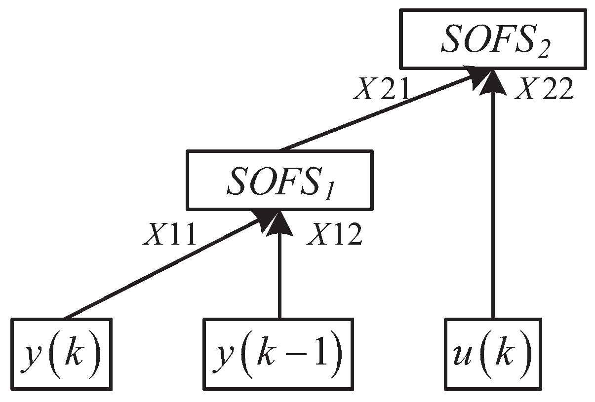
The basic structure of DHSOIT2FS is shown in Figure 1. The input and fuzzy systems for each layer are denoted as $X_{ij},{\mathrm{SOFS}}_k$, where i denotes the ith level, j denotes the jth input, and k denotes the kth sub-fuzzy system. Consider a problem with n-dimensional input and a single output. A DHSOIT2FS will contain $n-1$ SOFS subsystems. The entire system is constructed from the bottom up. This is a serial hierarchical structure that allows the system to be computationally reduced, the overall number of rules to be reduced, and the interpretability to be improved.

Each subsystem is a two-input, one-output system; thus, the number of rules and the number of fuzzy sets for a single sub-fuzzy system is not too large, and the computational complexity is low. For each subsystem, the desired output data are the desired output at the current moment. The input of the first sub-fuzzy system is the first two dimensions of input data at the current moment. The input of the subsequent sub-fuzzy system is the integration of the output of the previous sub-fuzzy system with the data of the next dimension.

The entire deep hierarchical fuzzy system is trained from the bottom to the top. Training processes with respect to the signal sub-fuzzy system is carried out as described above. The input and output data pairs are first obtained, and then the structure is learned, followed by the parameters, and the current output is finally given. This structure is suitable for use in online data streams. For each online data, each sub-fuzzy system is trained in turn until the entire system is trained. The entire process is quick and efficient. Then, the next data point is imported, and so on until all data streams are trained. This approach is different from using all training data to train a subsystem individually and then using all data to train the next subsystem.

4. Simulation

In this section, nonlinear dynamical system identification, high-dimensional dynamical system identification, and a single-link robot control problem are provided. The simulation results illustrate the effectiveness of the methods in this paper.

4.1. Nonlinear Dynamic System Identification

A simple nonlinear system is used to approximate a simple robotic system. Its expression is given in (22) and is widely used in several papers. It is used to verify the effectiveness of the algorithm proposed in this paper.

$$y(k+1)=\frac{y\left(k\right)y(k-1)\left[y\right(k)+2.5]}{1+y^2\left(k\right)+y^3(k-1)}+u\left(k\right)$$

(22)

where $u\left(k\right)=sin(2\pi k/25),y\left(0\right)=0,y\left(1\right)=1$. There are three inputs $\left(y\left(k\right),y(k-1),y\left(k\right)\right)$ and one output $y(k+1)$. The model can be described by the following equation:

$$y_p(k+1)=f\left(y\left(k\right),y(k-1),u\left(k\right)\right)$$

(23)

where $f(·)$ represents the fuzzy model obtained by our algorithm. Five hundred patterns are generated from $k=1$ to $k=500$, with the first 400 patterns used for training and the last 100 used for testing. The parameters in the DHSOIT2FS are set to be $f_{th}=0.1$, ${\sigma }_0=0.4$, and $\eta =0.001$. The RMSE between desired output $y_d(k+1)$ and predicted output $y_p(k+1)$ includes evaluation indicators, which is calculated as follows.

$$\mathrm{RMSE}=\sqrt{\frac{{\sum }_{k=400}^{499}{\left(y_d\left(k+1\right)-y_p\left(k+1\right)\right)}^2}{500}}$$

(24)

The structure of the system is shown in Figure 2. There are two sub-fuzzy systems, SOFS1 and SOFS2, and the output of the former system is used as the first dimensional input of the next system. The entire system is constructed using online data. After each piece of data comes in, it is first trained using $y\left(k\right)$ and $y(k-1)$ as the two-dimensional inputs to SOFS1. After the parameters of SOFS1 are adjusted, its output and $u\left(k\right)$ are used as two-dimensional inputs with respect to SOFS2 for training.

To better illustrate the effectiveness of the algorithm, a comparison is made here with the algorithm in the paper [26]. The algorithm uses the code provided in the attachment of the paper [26]. The number of fuzzy sets for each dimension is set to seven. There is a sliding window size of 3, i.e., three inputs per subsystem. This method of constructing a deep fuzzy system is a stacked approach, which is different from the serial approach in this paper. The former requires more rules and fuzzy sets. It can be observed that our predicted output almost coincides with the desired output. The number of rules used by the two methods, the number of fuzzy sets, and the final RMSE accuracy on the test set are shown in

Table 1. Comparison of the results of the two methods in 4.1.

Methods	WM	DHSOIT2FS
RMSE	0.0926	0.0476
Number of rules	343	20
Total number of fuzzy sets	21	20
TrainRunTime	0.1570 s	2.1560 s
TestRunTime	0.0342 s	0.1790 s

. It can be seen that the method in this paper uses fewer rules and several fuzzy sets to obtain improved accuracies. Here, the simulation time of the WM method is much smaller than the simulation time of the method in this paper. Because the WM method is not trained online but offline, the training test time is very short. Although the simulation time of our method is longer than that of the WM method, it is within an acceptable range.

Figure 3 shows the predicted output of our method and the expected output of the test samples. It can be seen that the method in this paper keeps track of the given output very well. The horizontal and vertical coordinates are a numerical quantity and have no physical meaning; thus, there are no units. In particular, the horizontal coordinate represents the sampling interval, which is also not a real sense of time.

Figure 4 shows the fuzzy set of the entire DHSOIT2FS. It can be seen that the fuzzy sets are well distributed and each fuzzy set has a suitable width. The overall interpretability is strong.

Figure 5 shows the changes in the fuzzy system’s parameters throughout the training process. It can be seen that both antecedent and consequent parameters converge quickly, which verifies the effectiveness of the method in this paper.

4.2. Higher Dimensional System Identification

A simple equation is used here to describe a robotic system. High-dimensional data are also used to model the multidimensional inputs to the robot. The system can be described by (25):

$$y\left(k\right)=\frac{{\sum }_{i=1}^{m}y(k-i)}{1+{\sum }_{i=1}^m{y}^2(k-i)}+u(k-1)$$

(25)

where $u\left(k\right)=sin(2\pi k/20),y\left(k\right)=0,k=1,2,\dots ,m$. In this paper, we take m as 10. There are ten inputs, $\left(y(k-1),y(k-2),\dots ,y(k-10),u(k-1)\right)$, and one output, $y\left(k\right)$. The model can be described by the following equation.

$$y_p(k+1)=f\left(y(k-1),\dots ,y(k-10),u(k-1)\right)$$

(26)

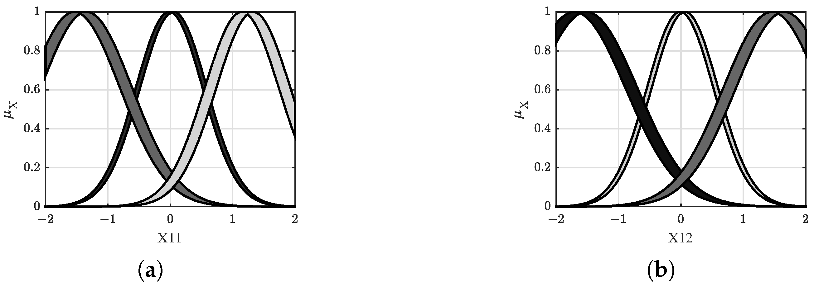
Three thousand three hundred patterns are generated from $k=1$ to $k=3300$, with eighty percent of the data used as the training set and the rest as the test set. The parameters in the DHSOIT2FS are set to be $f_{th}=0.01$, ${\sigma }_0=0.5$, and $\eta =0.001$. The evaluation metrics still use RMSE, and the formula is similar to (24). Training is also performed as described in the previous section. The structure of the system is similar to Figure 1. The method from the paper [26] is also used here for comparison. The number of its fuzzy sets is set to 5 and the size of the sliding window is set to 3. The number of rules used by the two methods, the number of fuzzy sets, and the final RMSE accuracy on the test set are shown in

Table 2. Comparison of the results of the two methods in 4.2.

Methods	WM	DHSOIT2FS
RMSE	0.2390	0.05185
Number of rules	3125	48
Total number of fuzzy sets	375	58
TrainRunTime	8.180 s	46.404 s
TestRunTime	2.159 s	4.457 s

. It can be seen that the method in this paper uses fewer rules and a number of fuzzy sets to obtain improved accuracies.

Figure 6 shows the predicted output of our method and the expected output of the test samples. It can be seen that the proposed method in this paper can identify nonlinear systems very well.

Figure 7 shows the fuzzy set of the SOFS1. The fuzzy sets are all distributed very evenly, and semantic variables can be specified for each fuzzy set. The system is highly interpretable.

4.3. Data-Driven Single Linkage Robot Control

Consider a single-link robot control system described by the following:

$$\begin{array}{r}M\ddot{q}+0.5\mathrm{mgl}sin\left(q\right)=\tau \\ y=q\end{array}$$

(27)

where M = 0.5 kgm${}^2$ represents the rotational inertia of the rod. m = 1 kg is the mass of the rod. l = 1 m denotes the length of the rod. g = 9.8 m/s${}^2$ stands for the acceleration of gravity. $q,\dot{q}$, and $\ddot{q}$ represent the angular position, angular velocity, and angular acceleration of the rod, respectively.

The task here is to consider keeping the angular position of the system constant at 1 (that is, to have the angular position of the system track a step signal). The simulation time is $ST$ = 5 s. The step size is 0.01. Assume that the initial states of the system are all zero. First, the pid control method is used with the following expression (28):

$$\tau \left(k\right)=k_{p}e\left(k\right)+k_i\sum _{n=0}^{k}e\left(i\right)+k_d\left(e\left(k\right)-e(k-1)\right)$$

(28)

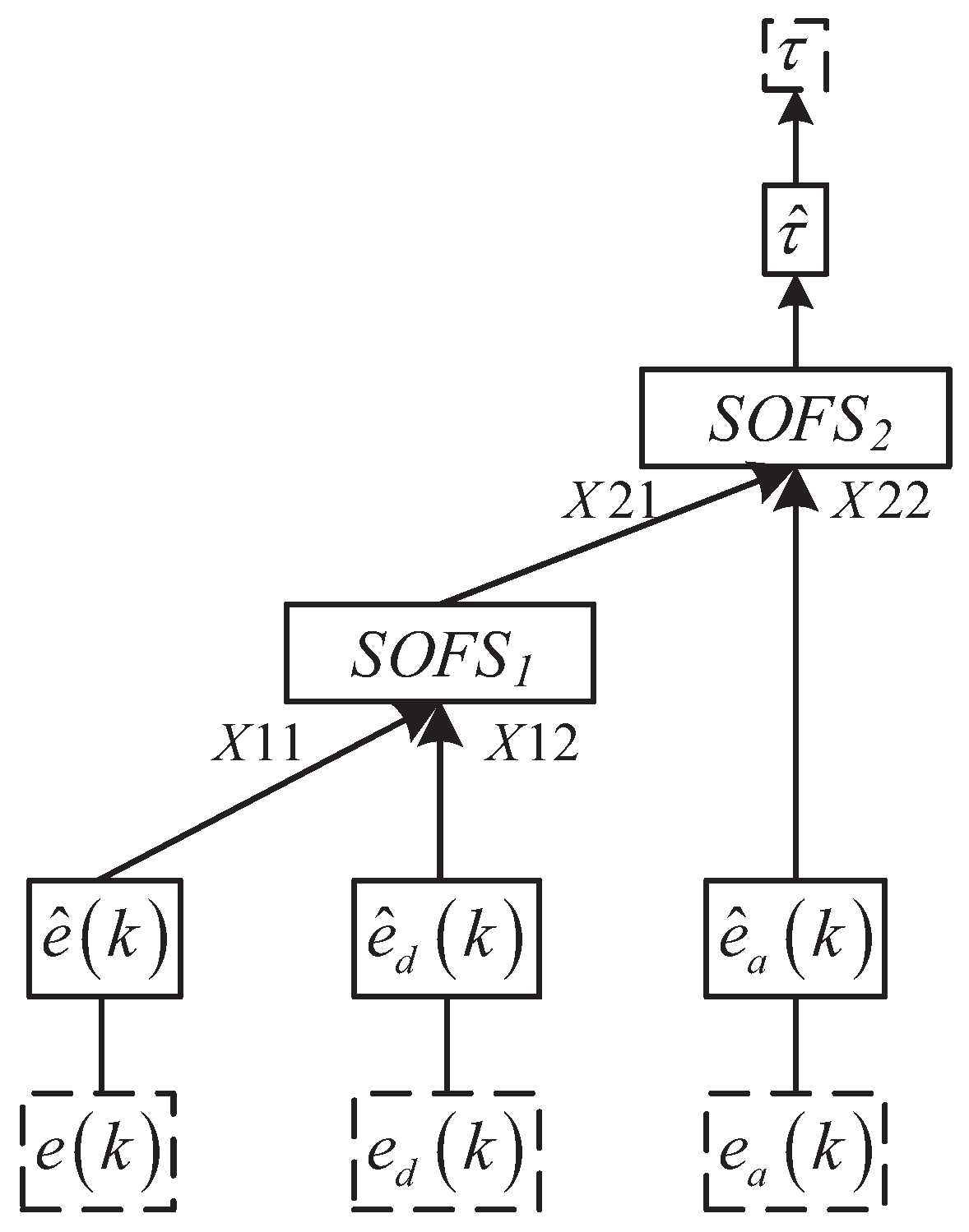
where $k_p$ is scale coefficient, $k_i$ is integral coefficient, and $k_d$ is differential coefficient. Appropriate pid parameters are selected, $k_p=100,k_i=5,k_d=2000$, to make the system stable. Moreover, define $e_a\left(k\right)={\sum }_{n=0}^{k}e\left(n\right)=e_a(k-1)+e\left(k\right),e_d\left(k\right)=e\left(k\right)-e(k-1)$. The composition of variables is inserted into input data sets $X=\left\{e\left(k\right),e_d\left(k\right),e_a\left(k\right),k=1,2,\dots ,4001\right\}$. The output data are the control signal $\tau \left(k\right)$. Since the order of magnitude of ea differs too much from that of e, two design approaches are considered here for normalizing and not normalizing the input and output data. This idea can also be extended to other data sets or control methods. The structure of the algorithm without normalization is similar to Figure 2. The normalized algorithm structure has two additional modules: the normalization of the input data and denormalization of the output data. The structure is shown in Figure 8, where variable $\widehat{e}\left(k\right),{\widehat{e}}_d\left(k\right),{\widehat{e}}_a\left(k\right),\widehat{\tau }$ is the normalized variable.

Since the data set needs to be collected first here, obtaining the maximum and minimum values of the data for the entire process is straightforward. Essentially, the online training method is still used here, with the exception that the prior knowledge of the maximum and minimum values of the inputs and outputs is known in advance. This is also available in practical applications. The normalized expressions are given below:

$$\widehat{e}\left(k\right)=\frac{e\left(k\right)-e_{min}}{e_{max}-e_{min}}$$

(29)

where $e_{min}$ and $e_{max}$ represent the minimum and maximum values of $e\left(k\right)$ in the entire training process, respectively. The parameters in the DHSOIT2FS are set to be $f_{th}=0.001$, ${\sigma }_0=0.4$, and $\eta =0.0001$. When the training is over, the resulting DHSOIT2FS is replaced by the pid controller in the original model. The result obtained is shown in Figure 9. $y1$ represents the output state obtained without the normalized DHSOIT2FS algorithm; $y2$ represents the output state obtained with the normalized DHSOIT2FS algorithm; $ypid$ represents the output state obtained with the pid algorithm; $yd$ represents the desired output state. The results of other methods are consistent with our method. The algorithm in this paper is completely data-driven, and there is no need to know any parameters of the model at all. In Figure 9, the lines of ypid are sources of the original data. Moreover, the method of this paper can well construct the fuzzy system after obtaining several data points, eventually making the effect consistent with it. This shows the effectiveness of the method in this paper because if the control method of the data source uses other methods with better controls, then the results of this paper can also fit that method very well. It can be seen that the output obtained by our method can track well on the given input, proving the effectiveness of our method.

Figure 10 shows the distribution of the fuzzy set of antecedent for the DHSOIT2FS algorithm with normalization. It can be seen that only one fuzzy set is used for each dimension. It is very concise as well as highly interpretable. In contrast, if the normalization algorithm is not used, the output of the SOFS1 sub-fuzzy system fluctuates greatly in value since it is trained using the desired control input, u. This would lead to a range of values of X21 well beyond [0,1], which would cause a mismatch between the parameters set by SOFS2 and the range of values of X21. This will cause the system to set too many unnecessary fuzzy sets as well as rules. This normalization method is the online learning method when the scope of the data is known. Although this experiment is a simple pid control simulation, the idea is analogous to other methods of the control simulation.

5. Conclusions

This paper proposes a new fuzzy system architecture: the DHSOIT2FS. Each sub-fuzzy system is a self-organizing interval type-2 fuzzy system, constructed online, with rules constructed by an online rule update algorithm, consequent parameters updated by iterative least squares, and antecedent parameters updated using a gradient descent algorithm. DHSOIT2FS uses a classic serial-layered structure to build the overall framework. The first layer uses the first two dimensions of data as input. Each subsequent layer uses the output of the previous layer with the next dimensional data as input until it is built. During the training process, each data point is trained with DHSOIT2FS before passing in the next data point to achieve the online construction. The effectiveness of the approach in this paper is illustrated using two numerical simulation examples as well as a robot control simulation example.

References

1. Ge, D.; Zeng, X.J. A self-evolving fuzzy system which learns dynamic threshold parameter by itself. IEEE Trans. Fuzzy Syst. 2018, 27, 1625–1637. [Google Scholar] [CrossRef] [Green Version]
2. Gu, X.; Shen, Q. A self-adaptive fuzzy learning system for streaming data prediction. Inf. Sci. 2021, 579, 623–647. [Google Scholar] [CrossRef]
3. Wei, Z.X.; Doctor, F.; Liu, Y.X.; Fan, S.Z.; Shieh, J.S. An optimized type-2 self-organizing fuzzy logic controller applied in anesthesia for propofol dosing to regulate BIS. IEEE Trans. Fuzzy Syst. 2020, 28, 1062–1072. [Google Scholar] [CrossRef]
4. Ferdaus, M.M.; Pratama, M.; Anavatti, S.G.; Garratt, M.A.; Pan, Y. Generic evolving self-organizing neuro-fuzzy control of bio-inspired unmanned aerial vehicles. IEEE Trans. Fuzzy Syst. 2019, 28, 1542–1556. [Google Scholar] [CrossRef] [Green Version]
5. Gu, X. Multilayer ensemble evolving fuzzy inference system. IEEE Trans. Fuzzy Syst. 2020, 29, 2425–2431. [Google Scholar] [CrossRef]
6. Zhao, T.; Tong, W.; Mao, Y. Hybrid Non-singleton Fuzzy Strong Tracking Kalman Filtering for High Precision Photoelectric Tracking System. IEEE Trans. Ind. Inform. 2022. [Google Scholar] [CrossRef]
7. Zhao, T.; Chen, C.; Cao, H. Evolutionary self-organizing fuzzy system using fuzzy-classification-based social learning particle swarm optimization. Inf. Sci. 2022, 606, 92–111. [Google Scholar] [CrossRef]
8. Zhao, T.; Cao, H.; Dian, S. A Self-Organized Method for a Hierarchical Fuzzy Logic System based on a Fuzzy Autoencoder. IEEE Trans. Fuzzy Syst. 2022. [Google Scholar] [CrossRef]
9. Zhao, T.; Chen, C.; Cao, H.; Dian, S.; Xie, X. Multiobjective Optimization Design of Interpretable Evolutionary Fuzzy Systems With Type Self-Organizing Learning of Fuzzy Sets. IEEE Trans. Fuzzy Syst. 2022. [Google Scholar] [CrossRef]
10. Karnik, N.N.; Mendel, J.M.; Liang, Q. Type-2 fuzzy logic systems. IEEE Trans. Fuzzy Syst. 1999, 7, 643–658. [Google Scholar] [CrossRef]
11. Mendel, J.M.; John, R.B. Type-2 fuzzy sets made simple. IEEE Trans. Fuzzy Syst. 2002, 10, 117–127. [Google Scholar] [CrossRef]
12. Deng, Z.; Choi, K.S.; Cao, L.; Wang, S. T2FELA: Type-2 fuzzy extreme learning algorithm for fast training of interval type-2 TSK fuzzy logic system. IEEE Trans. Neural Netw. Learn. Syst. 2013, 25, 664–676. [Google Scholar] [CrossRef] [PubMed]
13. Liang, Q.; Mendel, J.M. Interval type-2 fuzzy logic systems: Theory and design. IEEE Trans. Fuzzy Syst. 2000, 8, 535–550. [Google Scholar] [CrossRef] [Green Version]
14. Liang, Q.; Mendel, J.M. Equalization of nonlinear time-varying channels using type-2 fuzzy adaptive filters. IEEE Trans. Fuzzy Syst. 2000, 8, 551–563. [Google Scholar] [CrossRef] [Green Version]
15. Mitchell, H.B. Pattern recognition using type-II fuzzy sets. Inf. Sci. 2005, 170, 409–418. [Google Scholar] [CrossRef]
16. Yorozu, T.; Hirano, M.; Oka, K.; Tagawa, Y. Electron spectroscopy studies on magneto-optical media and plastic substrate interface. IEEE Transl. J. Magn. Jpn. 1987, 2, 740–741. [Google Scholar] [CrossRef]
17. Wang, L.X. Analysis and design of hierarchical fuzzy systems. IEEE Trans. Fuzzy Syst. 1999, 7, 617–624. [Google Scholar] [CrossRef]
18. Lee, M.L.; Chung, H.Y.; Yu, F.M. Modeling of hierarchical fuzzy systems. Fuzzy Sets Syst. 2003, 138, 343–361. [Google Scholar] [CrossRef]
19. Zhang, Y.; Ishibuchi, H.; Wang, S. Deep Takagi–Sugeno–Kang fuzzy classifier with shared linguistic fuzzy rules. IEEE Trans. Fuzzy Syst. 2017, 26, 1535–1549. [Google Scholar] [CrossRef]
20. Fukuda, T.; Hasegawa, Y.; Shimojima, K. Structure organization of hierarchical fuzzy model using by genetic algorithm. Proc. 1995 IEEE Int. Conf. Fuzzy Syst. 1995, 1, 295–300. [Google Scholar]
21. Hinton, G.E.; Osindero, S.; Teh, Y.W. A fast learning algorithm for deep belief nets. Neural Comput. 2006, 18, 1527–1554. [Google Scholar] [CrossRef]
22. LeCun, Y.; Bengio, Y.; Hinton, G. Deep learning. Nature 2015, 521, 436–444. [Google Scholar] [CrossRef] [PubMed]
23. Wang, G.; Qiao, J. An Efficient Self-Organizing Deep Fuzzy Neural Network for Nonlinear System Modeling. IEEE Trans. Fuzzy Syst. 2022, 30, 2170–2182. [Google Scholar] [CrossRef]
24. Silver, D.; Huang, A.; Maddison, C.J.; Guez, A.; Sifre, L.; Van Den Driessche, G.; Schrittwieser, J.; Antonoglou, I.; Panneershelvam, V.; Lanctot, M.; et al. Mastering the game of Go with deep neural networks and tree search. Nature 2016, 529, 484–489. [Google Scholar] [CrossRef]
25. Sadeghi, R.; Banerjee, T.; Romine, W. Early hospital mortality prediction using vital signals. Smart Health 2018, 9, 265–274. [Google Scholar] [CrossRef] [PubMed]
26. Wang, L.X. Fast Training Algorithms for Deep Convolutional Fuzzy Systems With Application to Stock Index Prediction. IEEE Trans. Fuzzy Syst. 2020, 28, 1301–1314. [Google Scholar] [CrossRef] [Green Version]
27. Qin, B.; Nojima, Y.; Ishibuchi, H.; Wang, S. Realizing deep high-order TSK fuzzy classifier by ensembling interpretable zero-order TSK fuzzy subclassifiers. IEEE Trans. Fuzzy Syst. 2020, 29, 3441–3455. [Google Scholar] [CrossRef]
28. Liu, Y.; Lu, X.; Peng, W.; Li, C.; Wang, H. Compression and regularized optimization of modules stacked residual deep fuzzy system with application to time series prediction. Inf. Sci. 2022, 608, 551–577. [Google Scholar] [CrossRef]
29. Juang, C.F.; Tsao, Y.W. A self-evolving interval type-2 fuzzy neural network with online structure and parameter learning. IEEE Trans. Fuzzy Syst. 2008, 16, 1411–1424. [Google Scholar] [CrossRef]
30. Mendel, J.M. Computing derivatives in interval type-2 fuzzy logic systems. IEEE Trans. Fuzzy Syst. 2004, 12, 84–98. [Google Scholar] [CrossRef]
Figure 1. The structure of the DHSOIT2FS.
Processes 10 02091 g001
Figure 2. The structure of the DHSOIT2FS in 4.1.
Processes 10 02091 g002
Figure 3. The predicted output with the desired output in 4.1.
Processes 10 02091 g003
Figure 4. Fuzzy set of the entire DHSOIT2FS in 4.1. (a) Fuzzy set of SOFS1’s first dimension. (b) Fuzzy set of SOFS1’s second dimension. (c) Fuzzy set of SOFS2’s first dimension. (d) Fuzzy set of SOFS2’s second dimension.
Processes 10 02091 g004
Figure 5. Variations in antecedent and consequent parameters during DHSOIT2FS training. (a) Antecedent parameters. (b) Consequent parameters.
Processes 10 02091 g005
Figure 6. The predicted output with the desired output in 4.2.
Processes 10 02091 g006
Figure 7. Fuzzy set of the SOFS1 in 4.2. (a) Fuzzy set of SOFS1’s first dimension. (b) Fuzzy set of SOFS1’s second dimension.
Processes 10 02091 g007
Figure 8. The structure of the DHSOIT2FS in 4.3.
Processes 10 02091 g008
Figure 9. The output obtained by each control algorithm and the desired output.
Processes 10 02091 g009
Figure 10. Distribution of the fuzzy set of antecedent for the DHSOIT2FS algorithm with normalization. (a) Fuzzy set of SOFS1’s first dimension. (b) Fuzzy set of SOFS1’s second dimension. (c) Fuzzy set of SOFS2’s first dimension. (d) Fuzzy set of SOFS2’s second dimension.
Processes 10 02091 g010