1. Introduction
Normally, allowing a vacation for a server helps to maintain the working efficiency and increase the life span of the server (machine). Due to continuously working in the system, even a human server may encounter physical or mental stress, which reduces their efficiency. As a result, the vacation allows the human server to de-stress and re-energize. After completing the vacation, the server can maintain the productivity of the system without any hardship. One can gain a deep understanding of a single server vacation under the queuing system by referring to Doshi [
1], Tian and Zhang [
2], and Ke et al. [
3].
The concept of vacation was first initiated in an inventory system by Daniel, and Ramanarayanan [
4] who applied the server vacation during the stock-out time. Sivakumar [
5] extended the multiple vacation policy in a retrial queuing inventory system. Jeganathan [
6] analyzed a finite queuing inventory system with multiple vacations of a single server and impatient customers whose reneging time is assumed to be exponential. Yadavalli and Jeganathan [
7] studied a retrial perishable inventory finite queuing system with two heterogeneous servers in which one server is assumed to take multiple vacations. Again, Jeganathan et al. [
8] explored the significance of heterogeneous servers over homogeneous servers on a finite retrial inventory system with server vacations.
Either during a period of stock out or a server vacation, any arriving customer’s demand is not fulfilled. Rather, some of their customers may revisit the shop/stall to meet their demand in the future due to the credibility of either of their products or services. This retrial concept plays an important role in the development of either queuing or inventory theory. The retrial concept with an inventory system was first studied by Artaljeo et al. [
9]. Paul Manuel et al. [
10] analyzed a retrial perishable inventory system with negative demands. Generally, we notice that the retrial of any individual customer does not depend on the other customers in orbit. However, the rate of retrial customers is directly proportional to the number of customers in orbit. An inventory system with this retrial policy is known as the classical retrial inventory system (CRIS). The analytical approach to CRIS was first established by Ushakumari [
11]. Krishnamoorthy and Jose [
12] studied a retrial inventory system in which the capacity of orbital customers is assumed to be infinite. Jeganathan et al. [
13], investigated a
retrial inventory system connected to a finite capacity waiting hall, where the service rate is queue dependent and a classical retrial policy is used for orbital customers. Recently, Jeganathan et al. [
14] studied a multi-server queueing inventory system with a classical retrial facility.
Dong-YuhYang et al. [
15] discussed a retrial queueing system with a single server that takes multiple optional vacations in a finite order under which batch arrivals and a constant retrial rate are also considered. Dong-Yuh Yang and Chia-Huang Wub [
16] described a finite capacity classical retrial queue with server breakdown in which the server is further encountered with working vacation under Bernoulli trail. Reshmi and Jose [
17] investigated a perishable inventory system with a classical retrial policy under a matrix analytic approach in which both primary and retrial customers were considered to enter into an orbit with independent Bernoulli’s schedules. Dhanya Shajin et al. [
18] deeply studied the marked Markovian arrival demand of a retrial inventory system with additional items and two kinds of customers where services are provided according to preemptive priority and threshold-based inventory, and classical retail policy is used for low priority customers with the Bernoulli approach. Jothivel Kathiresan et al. [
19] worked on a finite buffer inventory system with two kinds of services, and the nature of the service is assumed by Bernoulli distribution.
Most researchers have studied an inventory system where customers’ arrival policies are independent of stock levels in the system. Nevertheless, in a real-life scenario, the higher rate of customers entering happens in a system where the stock is kept in large quantities. This can be found at any marketplace where all dealers have kept their products in a line. Further, customers are inspired by a dealer who stocks their products in different sizes and modes in some conditions. For instance, in a food exhibition, a stall displays a food product with different varieties that attract different sections of people according to their age and diets. It is because the product choice varies according to customer preferences. Hence, customer preferences are highly satisfied by such a system with a large stock level. This will be seen on a regular basis at food exhibitions, book exhibitions, mobile showrooms, and car showrooms, among other places.
The following literature reviews show how the stock level influences the demand pattern of customers. Levin et al. [
20], Silver and Peterson [
21] both considered the number of customers’ arrivals functionally related to the quantity of displayed stock over a period of time. Gupta and Vrat [
22] defined the consummation rate of items as dependent upon the inventory size. Baker and Urban [
23] studied an inventory system with a deterministic approach where the demand is estimated as a polynomial function with the reference of stock level over the time interval. Badmanabhan and Vrat [
24] determined the optimum ordering quantity where the demand rate is assumed to be stock-dependent.
Further, Urban [
25] delineated and analyzed two kinds of demand rates, one of which is dependent upon the stock out period, and the other is dependent upon the stock-in period. Rathod and Bhathawala [
26] studied a stock-dependent inventory system with varying holding costs and shortages. Alfares [
27] deeply analyzed an inventory system where demand and storage time are assumed to be correlated with stock level and holding cost, respectively. Sudhir Kumar Sahu et al. [
28] discussed a perishable inventory system in which the demand rate is dependent upon the present stock level. Sandeep Kumar [
29] furnished the optimum ordering quantity and cycle time of a stock-dependent inventory system with shortages and variable holding costs.
Gabi Hanukov et al. [
30] also analyzed the stock-dependent Markovian demand with two servers. In this model, the preliminary service inventory is also made during the servers’ idle time. Jeganathan et al. [
31] analyzed the comparative study in their queueing-inventory system in which they assumed that the arrival process of a customer was dependent on the current stock level of the system. Recently, Abdul Reiyas and Jeganathan [
32] discussed stock-dependent arrivals in the base stock queueing-inventory system. Mostly, many authors applied a positive service time in their respective models, whereas Paul Manual et al. [
10], Sivakumar [
33], Sivakumar [
34], and Jeganathan et al. [
31] assumed that the inventory in the system was depleted at the instant of the arrival of a customer.
These observations strongly motivated us to do further research on an inventory system with stock-dependent arrivals. In the extension of Sivakumar [
5], the arrival of both primary and retrial is incorporated with the dependency of stock level, which makes the novelty of this study. In addition, we employ the classical retrial policy for a retrial customer. The rest of the paper is designed as follows. In the next section, the mathematical formulation of the model is explained. The details of the mathematical approach of the model with the steady-state analysis are presented in
Section 3. Furthermore, the analysis of waiting time is done in
Section 4. Some key system performance measures and sensitive analysis of the model are achieved in
Section 5 and
Section 6, respectively. Furthermore, the conclusion is given in the last section.
2. Explanation of System
This paper investigates a continuous review inventory to explore a stock-dependent arrival process for a customer and two different tasks for the server. This system can hold a maximum of S items. The server availability can be either in vacation mode or in normal mode (not on vacation). In this connection, the arriving customer receives an item immediately whenever the inventory is positive. More clearly, the customer’s service time is assumed to be instantaneous. In the event of a zero stock level, the server goes on vacation. If the server finds a positive inventory at the end of the vacation, then only he will return from the vacation; otherwise, (zero stock level), he will take another vacation. This is called the “multiple vacation policy”.
Any primary arrival of the system is assumed to be a non-homogeneous Poisson process. This is because the primary arrival to the system is dependent on the current stock level. The intensity rate of a primary arrival is defined as where . As we stated earlier, during the stock-out period, the server goes into vacation mode. In such a period (the server is on vacation), an arriving primary customer enters into an infinite orbit with an intensity . The customer from orbit can approach the system at any time. However, the successful retrial of a customer happens only when the inventory is not empty and the server is in normal mode. The time between two successful retrials is assumed to be exponentially distributed. The retrial process of a customer is dependent on the current stock level as well as the number of customers in the orbit. The intensity of a retrial customer is defined as , where k is the number of customers in the orbit and . Further, the replenishment process of the system will be started immediately if the inventory level falls to the predetermined stock level s under the ordering policy. The lead time follows an exponential distribution and its intensity is denoted as .
Description of Stock-Dependent Parameters
: mean retrial rate of orbital customers is given by , , , .
: mean arrival rate of primary customers is given by , , ,
3. Analysis of the System
This system can be referred by triplets , where and represent orbital customers’ size, server status and inventory level at time t, respectively.
The status of the server is defined by
Based on the assumptions of the given model, the continuous time discrete state random process
} is said to follow Markov process with the state space
E is determined by
and its infinitesimal generator transition rate matrix
M can be framed as:
Suppose be a transition state from a given state , then the following transition sub matrices are determined as follows:
Case (i):
The following sub-block holds the transition of a primary customer entering into orbit if the server is on vacation mode.
Case (ii):
The following sub-block holds the transition of a retrial customer who purchases the product successfully if the server is in normal mode.
For
Case (iii):
The following sub-block holds the transition of the reorder level, vacation return, primary and retrial customer is purchasing.
For
It is noted that the above matrices are all square matrices of order .
3.1. Matrix Geometric Approximation
Steady-State Analysis
Consider
k to be the cutoff point for the matrix-geometric approximation in the truncation process. Since the solving procedures of a classical retrial system have some analytical difficulty, we apply the Neuts-Rao truncation method. The classical retrial system under consideration is terminated at the truncation point
k. After such truncation point, the system admits a constant retrial policy for a retrial customer. This concept is called the Neuts-Rao truncation method. We assume
and
for all
. The modified generator matrix of the truncated system
is shown below.
3.2. Analysis of Steady-State Behavior
Let
. Then
N can also be determined by
where
Clearly N is a square matrix of order and the sub-matrices and are all matrices of orders and , respectively.
Lemma 1. The steady-state probability vector where = and = corresponding to the generator N is given bywhere,and can be obtained by solving equation and . Proof. Let be the steady-state probability vector of N. That is, satisfies .
The equation
of the above yields the following set of equations:
Now, expanding the Equations (
1) and (2) explicitly, we obtain the following set of equations,
Solving the above system of equations recursively and using the normalizing condition, we get the stated result. □
Next, we derive the condition under which the system is stable.
Lemma 2. The stability condition of the system under study is given by Proof. From the well known result of Neuts [
35] on the positive recurrence of
M we have
and by exploiting the structure of the matrices
and
and
the stated result follows. □
It can be seen from the structure of the rate matrix
M and from the Lemma 2, that the Markov process
with the state space
E is regular. Hence the limiting probability distribution
exists and is independent of the initial state. Let
satisfies
We can partition the vector
as
3.3. R Matrix Calculation
For analyzing the QBD process, suppose the steady-state probability vector can be determined by the relation
The rate matrix,
R, is the smallest non-negative solution to the quadratic equation above. Because the matrix
only has two non-zero rows, the structure of the unknown rate matrix
R also has two non-zero rows, resulting in a rate matrix
R with only non-zero entries in the first two rows and only zero elements in the remaining rows:
Apply R to the Equation (4), we get the following set of equations:
For
,
From the above non-linear equations, the matrix R can be determined explicitly by using Gauss–Seidel iterative technique.
Theorem 1. The vector Φ can be determined by due to the special structure of M and where R is as in Equation (4) and the vector and can be computed by set of equations Proof. The sub vector
and the block partitioned matrix of
gives the set of equations
using Equation (
8),
again using (
8),
where
Next,
where
On continuing this procedure up to
times, we get,
where
We use the block Gaussian elimination method to find the vectors
. The sub vector
satisfies the following relation,
Assume,
From (
10) we get
This can be written as
(
11) becomes
Since
= 1, then
As a result,
is the only solution to the Equations (
12) and (
13).
Hence,
Again by (
9) and (
14), we get (
6). Since
= 1 and using (
6),
which gives
as in (
7). □
6. Numerical Investigation
The author’s real-life experience is studied to provide a numerical picture for the readers regarding the contemplated recommended model. One day, the author went to a mobile store and observed how it operated. It also sells clients’ pen drives. Those who come into the shop to make a purchase are instantly served. They will not let a new customer into the system if there’s a zero-stock situation. They go outside and perform some personal work in such a situation. They return after some time to buy the pen-drive if it is still available. Suppose the shop has more pen drives. They start displaying or advertising them. When customers or people see the advertisement, they start purchasing. When the current stock level reaches some fixed quantity, the server makes a call to the supplier to furnish the replenishment. If there is no pen drive available currently, the server will close its service and take a rest. Once the ordered pen drive comes, the server will continue his service. From this experience, the author wanted to use the pen-drive sales functions as a mathematical model. Since the arrival occurs according to the displayed stock level, a stock-dependent arrival process is considered in this paper. At zero stock level, the server’s rest situation is considered a vacation, and new customers are not allowed. To provide a numerical illustration, an arrival rate (positive stock), , a reorder rate, , an arrival rate (zero stock), , a vacation completion rate, , scale factors, , a retrial rate, , a holding cost, , a setup cost, , and awaiting cost per unit in the orbit, are assumed.
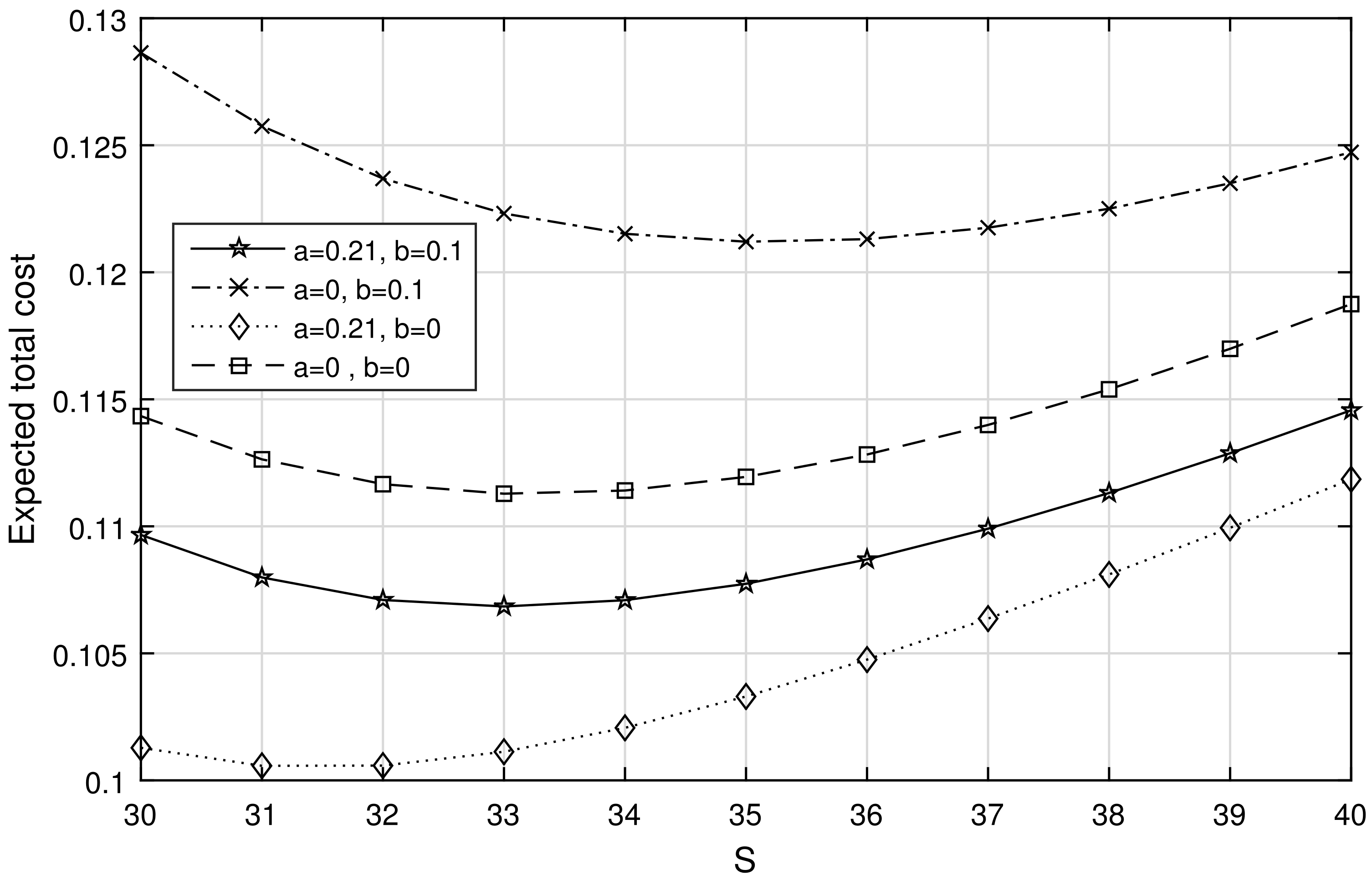
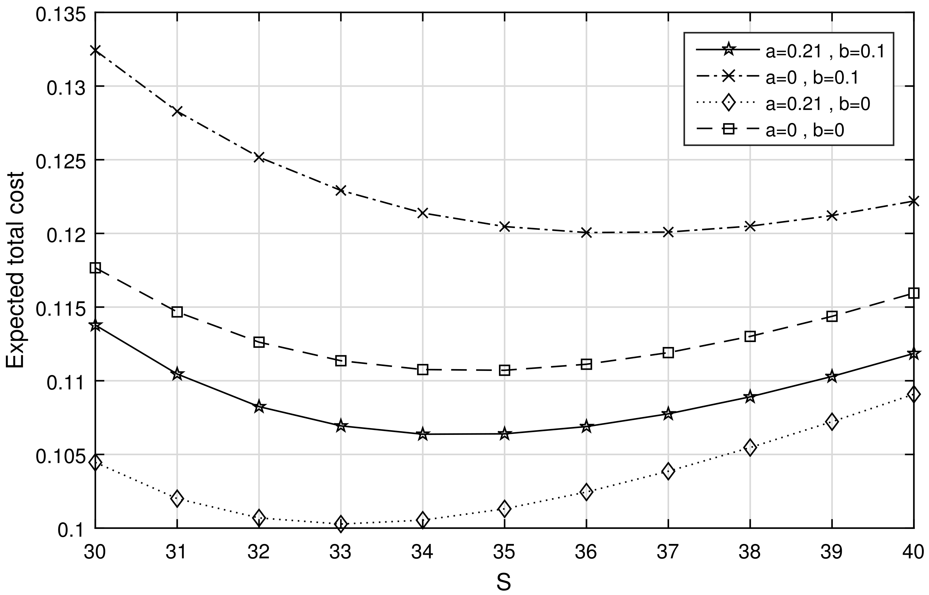
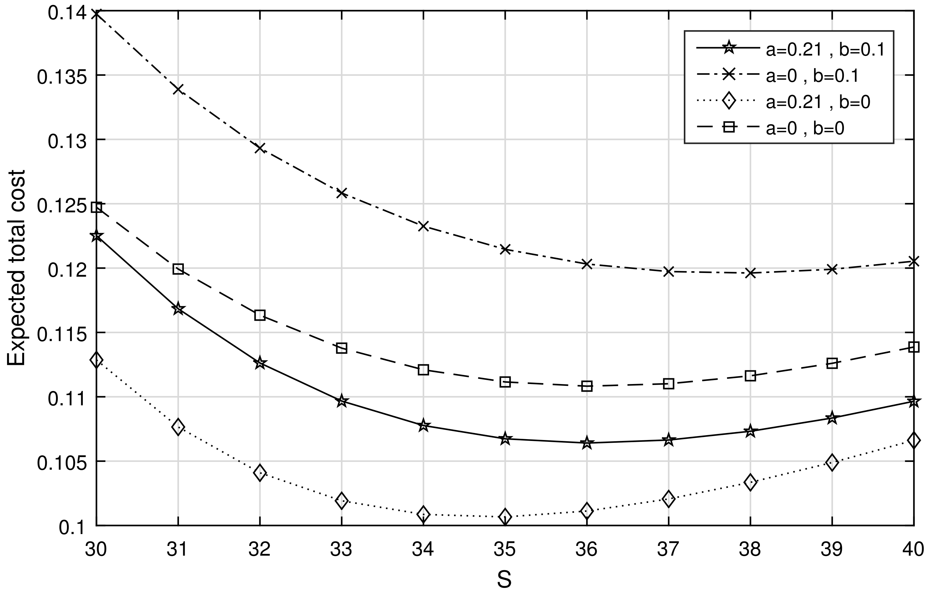
Case (i):
The two dimensional, local convexity of the expected total cost curve(
) is obtained when the maximum number of items(number of pen-drive)
S lies in the integer interval [30,40] with regard to pre-fixed reorder level
,
and
which are shown in
Figure 1,
Figure 2 and
Figure 3 respectively. Each figure depicts the convexity of the
curve under the classification of stock-dependent (SD) and non-stock-dependent (NSD). Each curve in those diagrams has a minimum point, which is referred to as the optimum point. That is, the estimated overall cost of pen-drive sales should be kept to a minimum (optimized). These curves show the total cost of the pen-drive sales when the arrival is wholly SD (
) and NSD (
) or partially SD (
,
and
,
). Because the optimum total cost is determined for both fully SD (or NSD) and partially SD arrivals, the organizer can pick for either the purely SD (or NSD) or partially SD arrival approach to boost pen-drive sales profits. The contrasting results of both solely and partially SD arrival processes are also shown in the
Figure 1,
Figure 2 and
Figure 3. This will be valuable to all readers as well as business tycoons who are in the inventory business (electric and electronic items, home appliances, etc.) and apply any of the arrival policies depending on their business plan. The optimal predicted total cost of the pen-drive store is attained when the store follows a partially SD arrival method, as shown in all three figures. However, if the
s varies, one can see that the best-reduced cost varies continually. They will determine the critical reorder level to attain the optimal
S, as indicated in
Figure 1,
Figure 2 and
Figure 3. Overall, at the middle reorder level
, the optimum estimated total cost of the pen-drive business exists. The overall expenditure of the store may be regulated with the help of this shown case, which shows the optimal predicted total cost of the pen-drive business and the best fit of the reorder point.
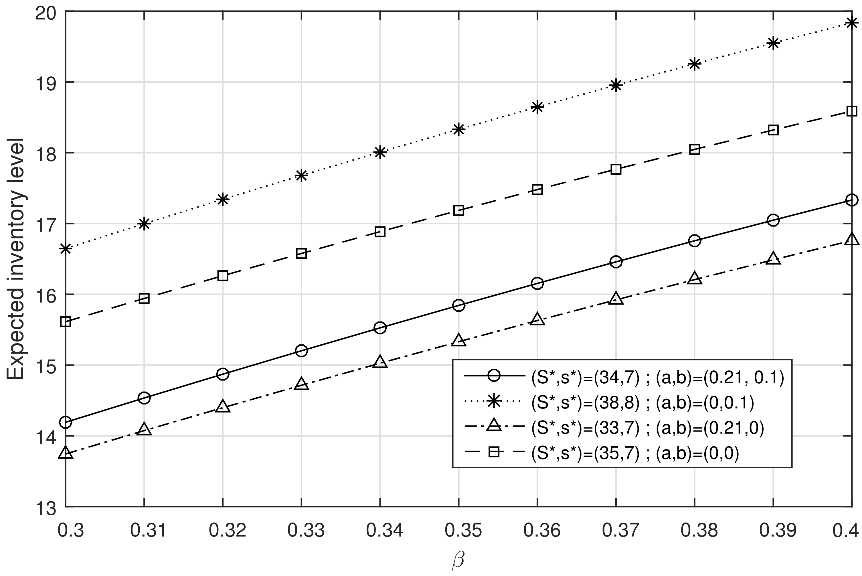
Case (ii):
This case explores the expected number of existing pen drives, its re-order rate, the number of customers in orbit, and the total and successful rate of retrial. With respect to purely SD (or NSD) and partially SD classifications. The increase in
shows that the average time between two consecutive reorders has decreased.
Figure 4 demonstrates that the expected number of current stock levels has increased if the lead time decreased. The owner of the pen-drive store will have more products in the storage system (if
is increased). That is, the shop’s displayed stock level has been increased. When individuals look at the objects on showcase, they may be tempted to them. They become customers and begin purchasing the displayed things if they are intrigued with them. The information concerning about expected reorder rate is shown in
Figure 5 which demonstrates that the re-order intensity rate is always proportional to its expected rate. As a result, as shown in
Figure 5, the merchant ensures that the appropriate steps are followed to obtain a prompt replacement.
Figure 6,
Figure 7 and
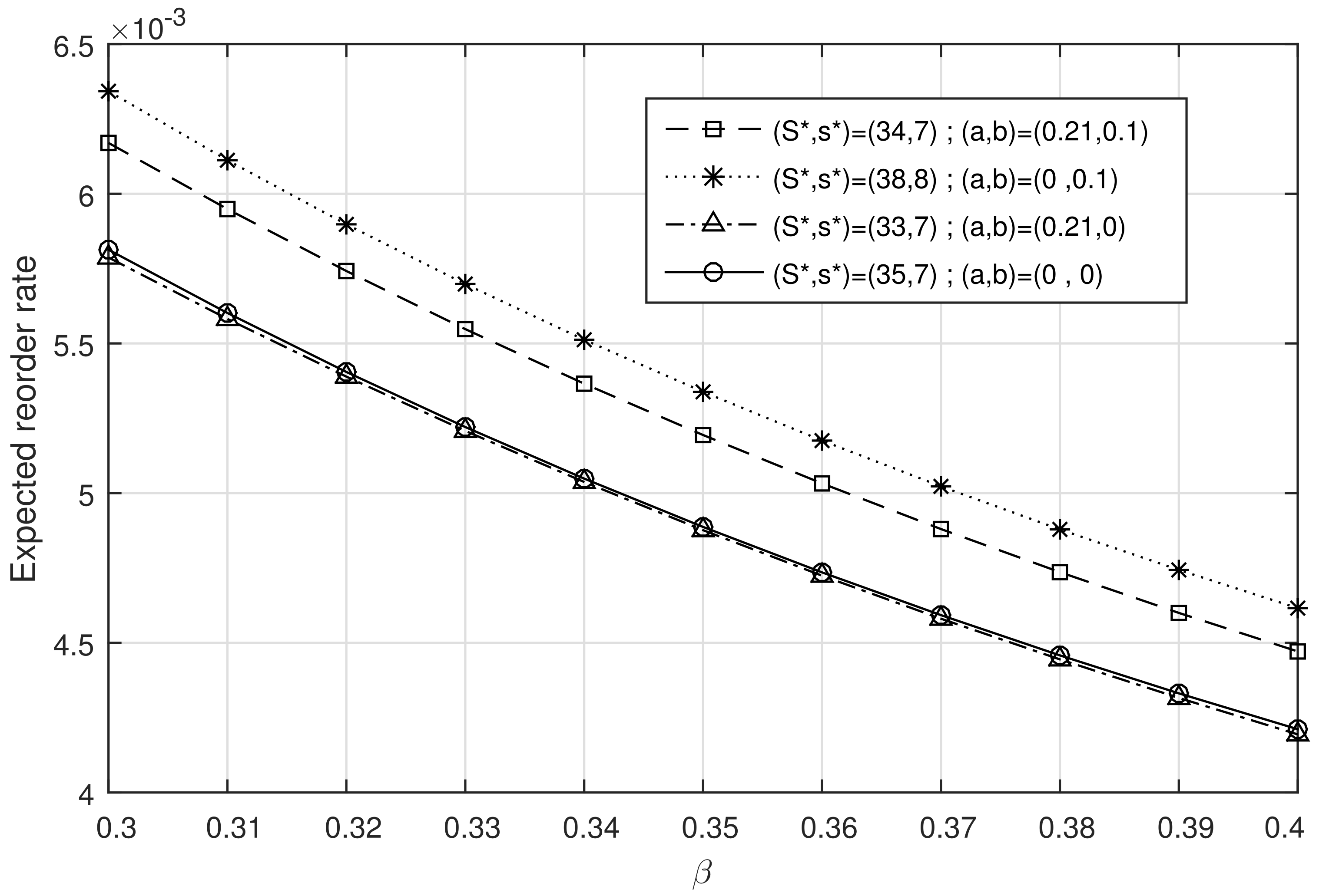
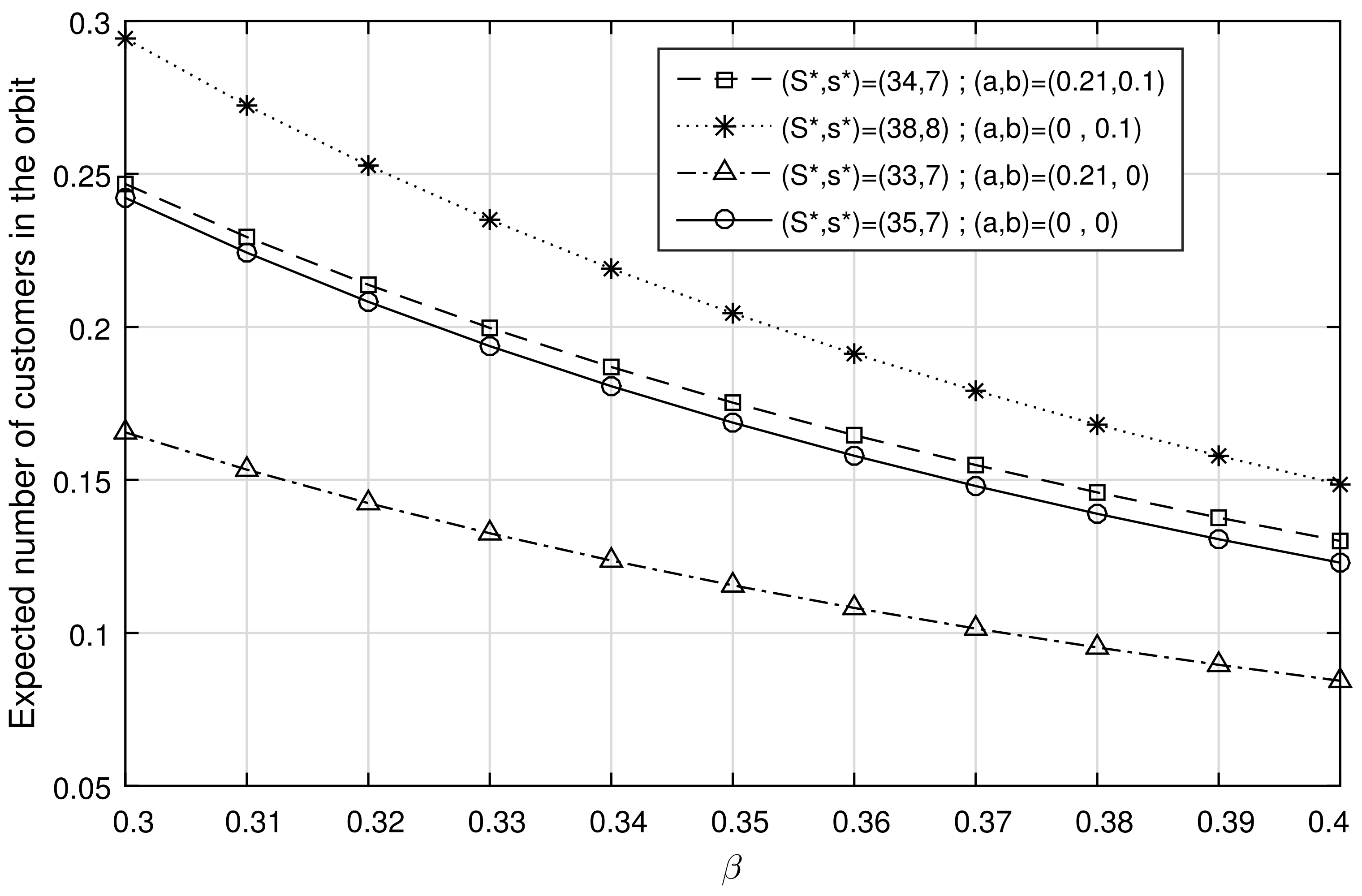
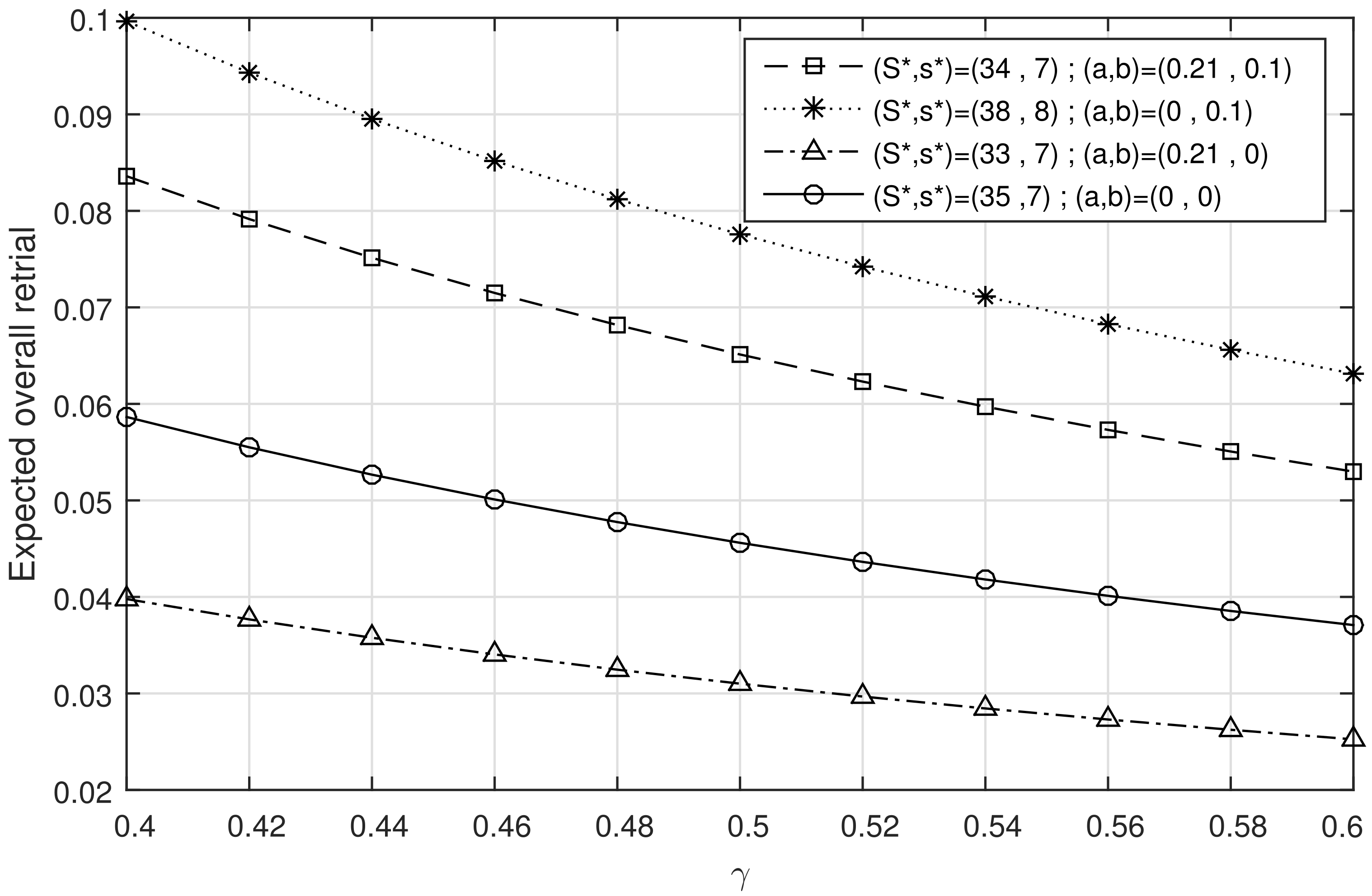
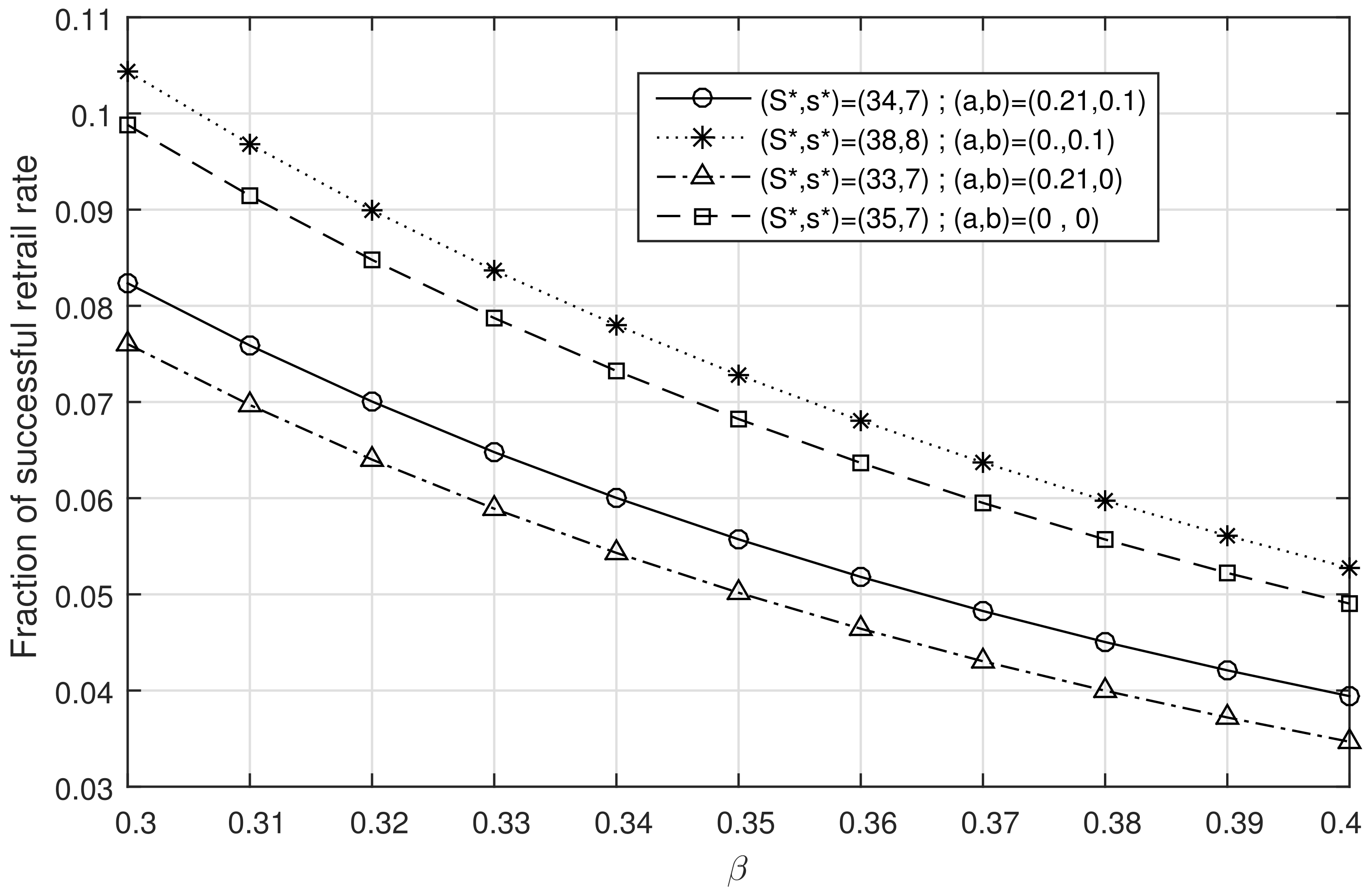
Figure 8 show the results as the lead time is inversely proportional to the number of customers in the orbit, the expected total, and the success rate of retrial customers, respectively. As previously stated, if
Q products are restocked quickly (i.e., if
is increased), the shop’s displayed stock level is likewise boosted. The boosting of the current stock level indicates the estimated number of consumers in orbit, the expected total retrial rate, and the expected successful retrial rate respectively. In the same way, the vacation will soon come to an end. As illustrated in
Figure 9,
Figure 10,
Figure 11,
Figure 12 and
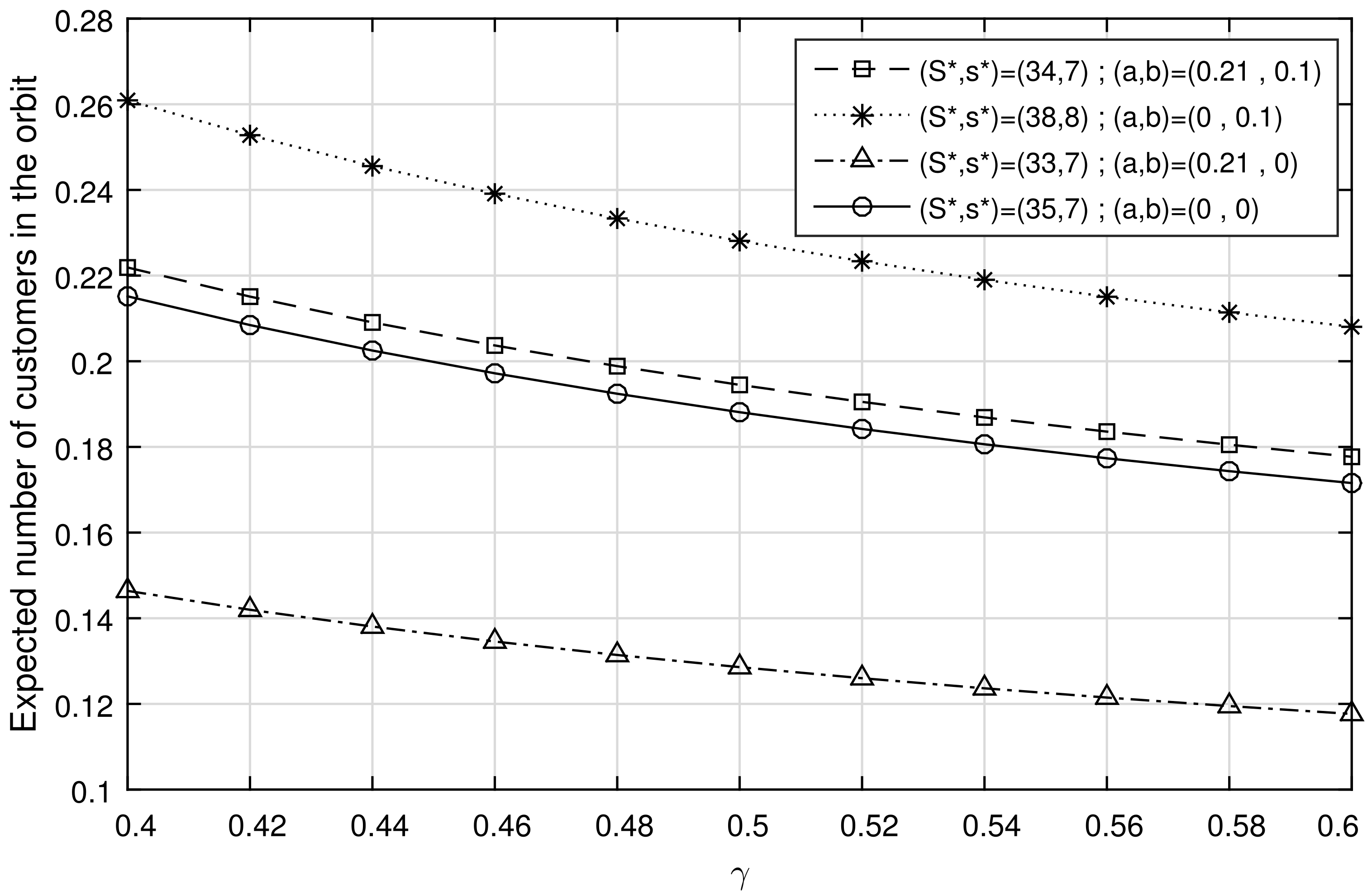
Figure 13 when the parameter
is increased, current stock level, expected reorder rate, average customer in the orbit, and their total and successful rate of retrial decrease. That means, if the pen-drive store owner spends as much time as possible on vacation, the measured metrics of the store’s performance will be impacted, as we predicted. This will assist them in deciding whether to lengthen or shorten their vacation time based on their preferences.
Case (iii):
The ideal total cost, optimal stock level, and optimal reorder level of the store are achieved by varying the cost values of waiting cost per customer, holding cost per item, and set-up cost per order together. From a business standpoint, cost functions are critical to making a profit. This explanation illustrates how changes in respective cost values affect the optimum number of pen drives that have to be stored, its re-order level, and predicted total cost. The store owner notices that the findings produced in
Table 1 demonstrate that the waiting cost per customer in the store and the set-up cost per order are both increased, and that the optimal stock, re-order levels, and predicted total cost are also increased. Based on these findings, the model’s assumed cost structure indicates that the store or firm should focus on calculating their cost values. If they lose control over the cost values, their total spending costs will rise and their profit will decrease. As a result of the cost function variation, the findings in
Table 1 show that if the store owner raises the holding cost per pen-drive, the calculated total cost rises. Similarly, the remaining set-up cost of the pen-drive for every order, as well as the waiting expenses per client in the orbit, drive up the total cost.
Case (iv):
In
Table 2,
Table 3,
Table 4 and
Table 5, under the parameter variation, optimum stock level, reorder level, total cost and expected inventory level, re-order rate, the average customer in the orbit are discussed. When we raise the arrival rate (both zero and positive stock or
and
) and the scale factors
a and
b and the retrial rate,
are proportional to optimum stock level, reorder level, total cost and expected, re-order rate, the average customer in the orbit separately. The number of customers entering the system per unit time has increased as the average arrival rate has increased. The system must stock a larger quantity of products in order to satisfy or give service to all of the arriving clients. If the current stock level falls below the reorder level quickly, the replenishment of
Q goods may be replaced promptly. If the replenishment does not take place right away, the current stock level will be depleted. Any arriving customer who discovers that the inventory level is empty may be sent into orbit. The scaling factors
a and
b perform the same function as
. On the other hand, the re-order intensity rate,
influences the measures optimum stock level, reorder level, total cost and expected inventory level, re-order rate, the average customer in the orbit in the inverse direction. This is because the existing stock level of the system is increased if the replenishment time is reduced. Since the re-ordered quantities arrive quickly, the store owner can provide the service as much as possible. If the service completion is to be done fast, the estimated measures taken into this case are to be decreased. Similarly, the vacation completion time (if
is increased) ends as soon as the server starts his work immediately. Suppose the customer finds that the server is in working mode, the number of the customer going to orbit will reduce. On following that the optimum stock and reorder level also decreased. In addition, the orbital customers also get the opportunity to get a quicker service. So that the customers expected total and successive retrial rates are reduced. This illustration inspires the readers to develop the stock-dependent arrival strategy in their business. Many businesses nowadays use social media to display their products in the most efficient way in order to enhance client traffic. The expansion and development of the inventory industry will be aided by such arrival dependencies.


 ,
, 


