Analysis and Assessment of Controllability of an Expressive Deep Learning-Based TTS System

Abstract

In this paper, we study the controllability of an Expressive TTS system trained on a dataset for a continuous control. The dataset is the Blizzard 2013 dataset based on audiobooks read by a female speaker containing a great variability in styles and expressiveness. Controllability is evaluated with both an objective and a subjective experiment. The objective assessment is based on a measure of correlation between acoustic features and the dimensions of the latent space representing expressiveness. The subjective assessment is based on a perceptual experiment in which users are shown an interface for Controllable Expressive TTS and asked to retrieve a synthetic utterance whose expressiveness subjectively corresponds to that a reference utterance.

1. Introduction

Text-To-Speech (TTS) frameworks, which generate speech from textual information, have been around for a few decades and have improved lately with the coming of new AI methods, e.g., Deep Neural Networks (DNN). Commercial products provide user-friendly DNN-based speech synthesis systems. Such recent systems offer an excellent quality of speech obtained by analyzing tens of hours of neutral speech, which often fail to convey any emotional contents. The task being examined by scientists today has evolved towards the field of expressive speech synthesis [1,2].

The aim of this task is to create not an average voice, but specific voices, with particular grain and extraordinary potential with regards to expressiveness. This will make it possible to make virtual agents behave in a characteristic way and hence to improve the nature of the interaction with a machine, by getting closer to human–human interaction. It remains to find good ways to control such expressiveness characteristics.

The paper is organized as follows:

• Related work is presented in Section 2;
• Section 3.2 describes the proposed system for controllable expressive speech synthesis; Section 4 presents the methodology that allows for discovering the trends of audio features in the latent space;
• Section 5 presents objective results using this methodology and results regarding the acoustic quality with measures of errors between generated acoustic features and ground truth;
• The procedure and results of the perceptual experiment is described in Section 6;
• Finally, we conclude and detail our plans for future work in Section 7.
  To obtain the results of the experiments of this paper, the software presented in [3] was used. It is available online (https://github.com/noetits/ICE-Talk, accessed on 29 August 2021) A code capsule (https://doi.org/10.24433/CO.1645822.v1, accessed on 29 August 2021) provides an example of use of the software with LJ-speech dataset [4] which in the public domain.

2. Related Work and Challenges

The voice quality and the number of control parameters depend on the synthesis technique used [1,5]. These parameters allow variations to be created in the voice. The number of parameters is subsequently important for the generation of expressive speech.

Historically, there have been different approaches to expressive speech synthesis. Formant synthesis can control numerous parameters; however, the generated voice is unnatural. Synthesizers using the concatenation of voice segments reach a higher naturalness; however, this technique provides few control possibilities.

The first statistical approaches using Hidden Markov Models (HMMs) [6] allows one to achieve both a fair naturalness and a control of numerous parameters [7]. The latest statistical approaches use DNN [8] and was the premise of new speech synthesis frameworks, for example, WaveNet [9] and Tacotron [10], referred to as Deep Learning-based TTS.

Regarding the controllable part of TTS frameworks, a significant issue is the labeling of speech information with style or emotion data. Late investigations have been directed into unsupervised strategies for how to accomplish expressive speech synthesis without the need for annotations.

A task related to controllable expressive speech synthesis is the prosody transfer task for which the goal is to synthesize speech from text with a prosody similar to another audio reference. A common characteristic of both tasks is the need for a representation of expressiveness. However, for controllable speech synthesis, this representation should be a good summary of expressiveness information; i.e., it should be interpretable. A low dimension would help the interpretability. For prosody transfer, the representation should be as accurate and precise as possible.

In [11], the authors present a prosody transfer system extending the Tacotron speech synthesis architecture. This extension learns a latent embedding space by encoding audio into a vector that conditions Tacotron along with the text representation. These latent embeddings model the remaining variation in speech signals after accounting for variation due to phonetics, speaker identity, and channel effects.

The authors of [12] propose a supervised approach that use a time-dependent prosody representation based on F0 and the first mel-generalized ceptral coefficient (representing energy). A dedicated attention module and a VAE are leveraged to enable the concatenation of information to linguistic encodings. This allows for a fine-grained prosody transfer instead of a sentence-level prosody information.

CopyCat [13] addresses the problem of speaker leakage in many-to-many prosody transfer. This problem occurs when the voice of the reference sample can be heard in the resulting synthesized speech, and it should only transfer prosody and not speaker identity. They are able to reduce the phenomenon with a novel reference encoder architecture that captures temporal prosodic representations robust to speaker leakage.

Concerning controllable speech synthesis, Ref. [14] proposed using a VAE and deploying a speech synthesis system that combines VAE with VoiceLoop [15]. Some other researches have used the concept of VAE [16,17] for controllable speech synthesis. In [16], the authors combine VAE and GMM and call it GMVAE. For more details concerning the different variants of such methods, an in-depth study of methods for unsupervised learning of control in speech synthesis is given in [17]. These works show that it is possible to build a latent space leading to variables that can be used to control the style of synthesized speech.

In [18], the authors show an example of spectrograms corresponding to a text synthesized with different rhythms, speaking rates, and F0. However, these works do not provide insights about the relationships between the computed latent spaces and the controllable audio characteristics.

Different supervised approaches were also proposed to control specific characteristics of expressiveness [19,20,21]. In these approaches, it is necessary to make a choice of control parameters a priori, such as pitch, pitch range, phone duration, energy, and spectral tilt. This reduces the possibilities of the controllability of the speech synthesis system.

A shortcoming of these investigations is that they do not give insights about the extent to which the system is controllable from objective and subjective points of view. We intend to fill this gap.

3. System

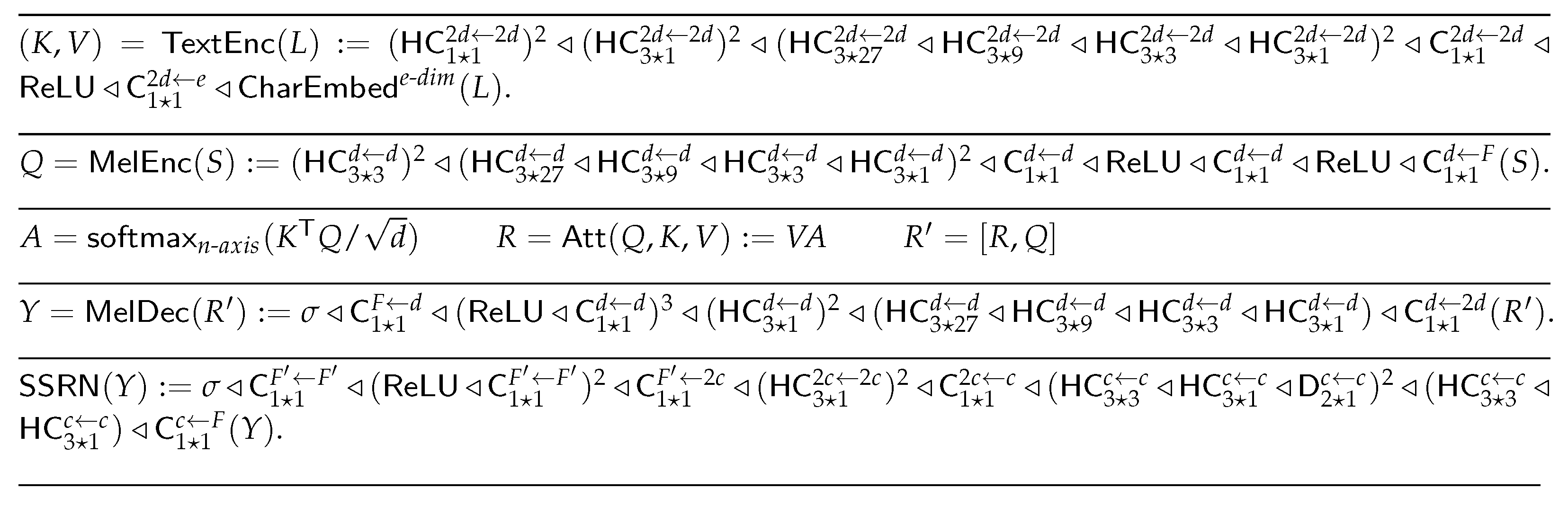
3.1. DCTTS

As our system relies on DCTTS [22], the details of the different blocks are given in Figure 1. We use the notations introduced in [22] in which the reader can find more details if needed.

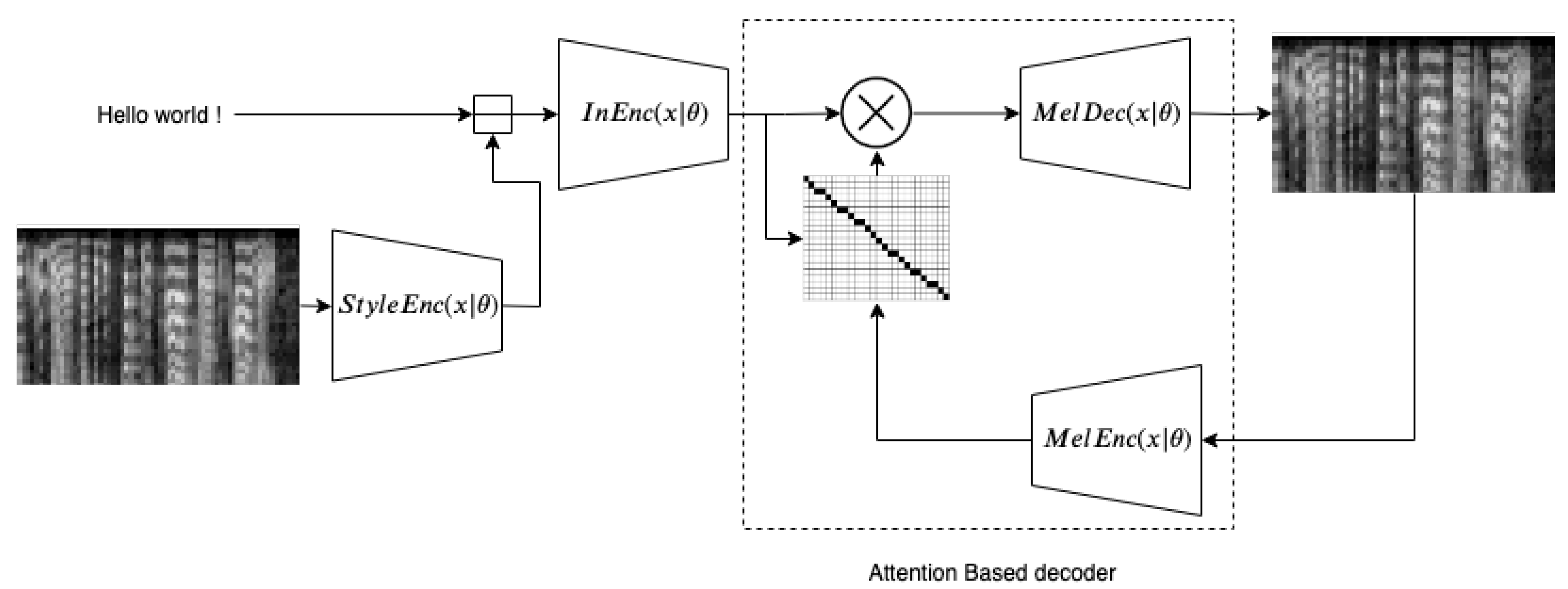
3.2. Controllable Expressive TTS

The system is a Deep Learning-based TTS system that was modified to enable a control of acoustic features through a latent representation. It is based on the Deep Convolutional TTS (DCTTS) system [22].

Figure 2 shows a diagram of the whole system. The basis DCTTS system constitutes the $InEnc$, the attention-based decoder comprising $MelEnc$ and $MelDec$.

For the latent space design, the $StyleEnc$ network was added. It consists of a stack of 1D convolutional layers similar to the $MelEnc$, followed by an average pooling. This operation enforces encoding time independent information. It can thus contain information about statistics of prosody such as pitch average and average speaking rate but not a pitch evolution. The latent vector at the output is the representation of expressiveness. This vector is then broadcast-concatenated to the character embedding matrix, i.e., repeated N times to fit embedding matrix length and then concatenated to it.

This system was compared to another in [23]. This comparison was done by training the system with a single speaker dataset with several speaking styles given by an actor and recorded in studio.

In this paper, we study the control of this system trained on the dataset with which we hope will enable a continuous control of expressiveness. The dataset is the Blizzard2013 dataset (https://www.cstr.ed.ac.uk/projects/blizzard/2013/lessac_blizzard2013/, accessed on 29 August 2021) by Catherine Byers based on an audio book with a great variability in vocal expressions and therefore in acoustic features.

The latent space is designed to represent this acoustic variability and as a control to the output. It allows this without any annotation regarding the expressiveness, emotion, and style because the representation is learned during the training of the architecture.

4. Post-Analysis for Interpretation of Latent Spaces

In this section, we explain the method presented in [23]. The methodology allows the trends to be discovered in the latent space. It can be done in the original latent space or in a reduced version of it.

The goal is to map mel-spectrograms into a space which is hopefully organized to represent the acoustic variability of the speech dataset.

To analyze the trends of acoustic features in latent spaces, we compute the direction of greatest variation in the space. For each feature of a set, we perform a linear regression using the point in the latent space and the feature computed from the corresponding file in the dataset.

The steps are the following:

• The mel-spectrogram is encoded to a vector of length 8 that contains expressiveness information. This vector is computed for each utterance of the dataset.
• Dimensonality reduction is used to have an ensemble of 2D vectors instead. Figure 3 shows a scatter plot of these 2D points.
• Then a trend is extracted for each audio feature. For, e.g., $F{0}_{mean}$, its value is computed for each utterance of the dataset. We therefore obtain an $F{0}_{mean}$ corresponding to each 2D-point $(x,y)$ of the scatter plot.
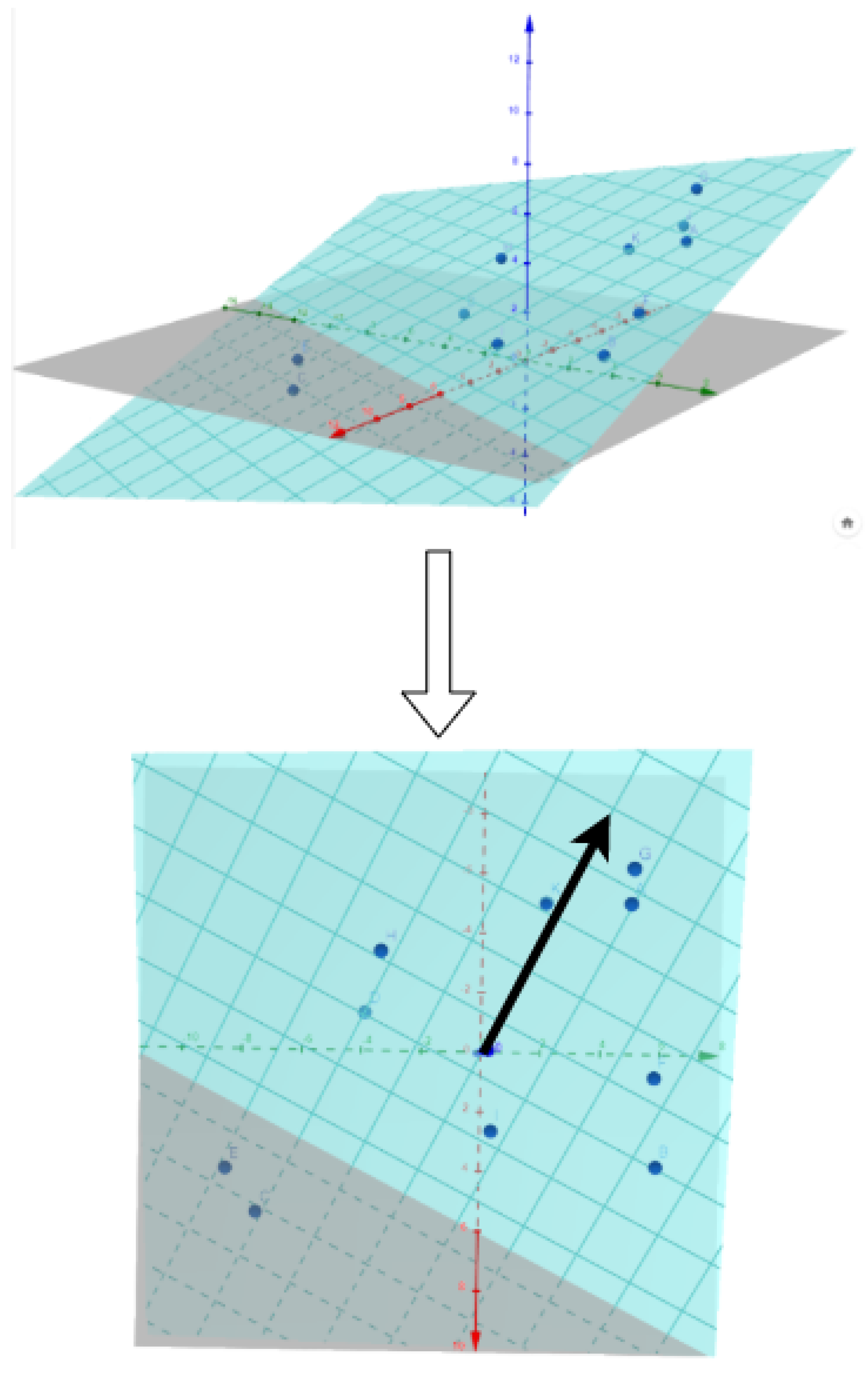
• We approximate the plane

  $$F0=f(x,y)=ax+by+c$$
• To assess that this plane $f(x,y)$ is a good approximation of $F{0}_{mean}$, implying a linear relation between a direction of the space and $F{0}_{mean}$, we compute the correlation between the approximations $f(x,y)$ with the ground truth values of $F{0}_{mean}$.
• If we compute the gradient of the plane (which is in fact $(a,b)$), we have the direction of the greatest slope, which is plotted in blue.

This representation is useful for a perspective of interface for controllable speech synthesis system on which are represented the trends of audio features in the space.

5. Objective Experiments

First we follow the methodology presented in the previous section to extract the directions in the latent space corresponding to acoustic features of eGeMAPS feature set [24] and quantify to which extent they are related by computing an Absolute Pearson Correlation Coefficient (APCC).

This feature set is based on low-level descriptors (F0, formants, mfcc, etc.) to which statistics for the utterance (mean, normalized standard deviation, percentiles) are applied. All functionals are applied to voiced regions only (non-zero F0). For MFCCs, there is also a version applied to all regions (voiced and unvoiced).

These features are defined in [24] as follows:

• F0: logarithmic F0 on a semitone frequency scale, starting at 27.5 Hz (semitone 0)
• F1–3: Formants one to three center frequencies
• Alpha Ratio: ratio of the summed energy from 50 to 1000 Hz and 1–5 kHz
• Hammarberg Index: ratio of the strongest energy peak in the 0–2 kHz region to the strongest peak in the 2–5 kHz region.
• Spectral Slope 0–500 Hz and 500–1500 Hz: linear regression slope of the logarithmic power spectrum within the two given bands.
• mfcc1–4: Mel-Frequency Cepstral Coefficients 1 to 4

To objectively measure the ability of the system to control voice characteristics, we do a sampling in the latent spaces and verify that the directions control what we want them to control.

Then we assess the quality of the synthesis using some objective measures.

5.1. Quantitative Analysis

5.1.1. Correlation Analysis

To visualize acoustic trends, it would be useful to have a small number of features that gives a good overview. To extract a subset of the list, we apply a feature selection with a filtering method based on Pearson’s correlation coefficient. The idea is to investigate correlations between audio features themselves to exclude redundant features and select a subset.

The steps are the following:

• Features are sorted by APCC in decreasing order;
• For each feature, APCC with previous features are computed;
• If the maximum of these $inter-features-APCCs>0.8$, the feature is eliminated;
• Finally, only features that have a $prediction-APCC>0.3$ are kept.

These limits are arbitrary and can be changed to filter more or fewer features from the list.

In

Table 1. APCC values between the best possible hyperplane of the latent space and audio features of the eGeMAPS feature set.

	APCC
F0 percentile50.0	0.723824
mfcc1V mean	0.619622
mfcc1 mean	0.554794
logRelF0-H1-A3 mean	0.493066
mfcc4V mean	0.492359
HNRdBACF mean	0.482579
F1amplitudeLogRelF0 mean	0.473154
slopeV0-500 mean	0.420381
StddevVoicedSegmentLengthSec	0.388952
F3amplitudeLogRelF0 stddevNorm	0.360528
mfcc2V mean	0.360144
hammarbergIndexV mean	0.356113
mfcc1V stddevNorm	0.350918
loudness meanFallingSlope	0.350369
loudness percentile20.0	0.340973
loudness meanRisingSlope	0.323489
F1frequency mean	0.318096

, we show the results of the APCC for Blizzard dataset. It can be noted that F0 median is the most predictable feature from the latent space. The feature selection method highlight a set of 17 diverse features that have an APCC $>0.3$.

5.1.2. Distortion Analysis: A Comparison with Typical Seq2seq

To compare the synthesis performance of the proposed method with a typical seq2seq method, we compare objective measures used in expressive speech synthesis. These measures compute an error between acoustic features of a reference and a prediction of the model. There exist different types of objective measures that intend to quantify the distortion induced by a system of audio quality or prosody. In this work, we use the following objective measures:

• MCD [25] measuring speech quality:
  ${\mathrm{MCD}}_K=\frac{1}{T}{\sum }_{t=0}^{T-1}\sqrt{{\sum }_{k=1}^K{\left(c_{t,k}-c_{t,k}^{\prime }\right)}^2}$
• VDE [26]: $\mathrm{VDE}=\frac{{\sum }_{t=0}^{T-1}1[v_t\ne v_t^{\prime }]}{T}$
• F0 MSE measuring a distance between F0 contours of prediction and ground truth:
  $\mathrm{F}0\_\mathrm{MSE}=\frac{1}{T}{\sum }_{t=0}^{T-1}{\left(F_{0t}-F_{0t}^{\prime }\right)}^2$
• lF0 MSE, similar to previous one in logarithmic scale:
  $\mathrm{lF}0\_\mathrm{MSE}=\frac{1}{T}{\sum }_{t=0}^{T-1}{\left(log{F}_{0t}-log{F}_{0t}^{\prime }\right)}^2$

Some works use DTW to align acoustic features before computing a distance. The problem with this method is that it modifies the rhythm and speed of the sentence. However, computing a distance on acoustic features that are shifted completely distorts the results; therefore, it is needed to apply a translation on acoustic features and take the smallest possible distance. We thus report measures with DTW and with only shift in

Table 2. Objective measures for the typical TTS system.

	MCD	VDE	lF0_MSE	F0_MSE
DTW	9.973914	0.015488	0.436348	1219.128507
shift	13.331841	0.236024	6.283607	9481.103150

for the original DCTTS and

Table 3. Objective measures for the proposed Unsupervised TTS system.

	MCD	VDE	lF0_MSE	F0_MSE
DTW	9.624296	0.009699	0.311803	957.290498
shift	12.675999	0.218258	5.838526	8931.599942

for the proposed unsupervised version of DCTTS.

5.2. Qualitative Analysis

In Figure 4, we show a scatter plot of the reduced latent space with the feature gradients. Each point corresponds to one utterance encoding and reduced to two dimensions. The color of these points is mapped to the values of an acoustic feature to be able to visualize how the gradients are linked to the evolution of the acoustic features. Two examples are shown for F0 median and standard deviation of voiced segment length, i.e., the duration of voiced sounds, which is linked to the speaking rate.

We can observe that the direction of the gradients follows well the general trend of the corresponding acoustic feature. As the correlation values indicate, F0 median has an evolution closer to a linear evolution in the direction of the gradient rather than for voiced segment lengths standard deviation.

6. Subjective Experiment

6.1. Methodology

An experiment was designed to assess the extent to which participants would be able to produce a desired expressiveness for a synthesized utterance, i.e., a methodology for evaluating the controllability of the expressiveness.

For this purpose, participants were asked to use the 2D interface to produce the same expressiveness as in a given reference. We assume that if participants are able to locate in the space the expressiveness corresponding to the reference, it means they are able to use this interface to find the expressiveness they have in mind.

The experiment contains two variants: in the first, the text of the reference and 2D space sentences are the same, while in the second, they are different. In the first one, the participant can rely on the intonation and specific details of a sentence, while in the second, he has to use a more abstract notion of expressiveness of a sentence.

The experiment is designed to avoid choosing a set of different characteristics or style categories and letting the participant of the experiment judge how close the vocal characteristics of a synthesized sentence is to a reference.

The procedure for preparing the experiment is as follows:

• The model trained with Blizzard2013 dataset is used to generate a latent space with continuous variations of expressiveness as presented in Section 3.2.
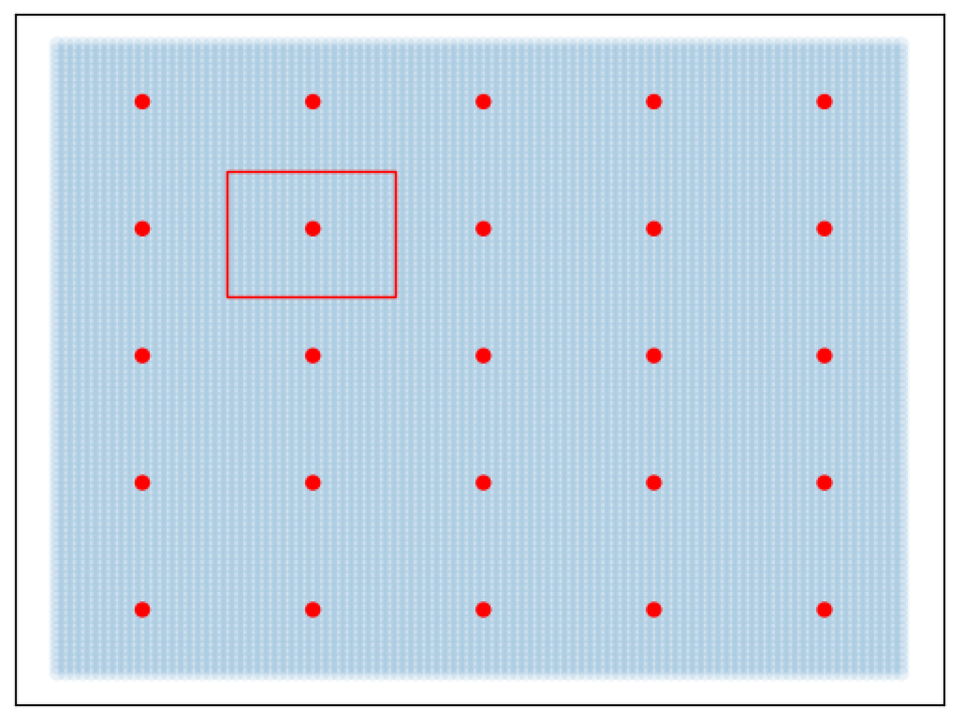
• In the 2D interface, we sample a set of points inside the region of the space in which the dataset points are located. The limits of the rectangle are defined by projecting sentences of the whole dataset in the 2D space with PCA and selecting $x_{min}$, $x_{max}$, $y_{min}$, and $y_{max}$ of all points. In other words, we use the smallest rectangle containing the dataset points. We use a resolution of 100 for x and y axes, making a total of 10,000 points in the space.
• This set of 2D points is projected to the 8D latent space of the trained unsupervised model with inverse PCA. The 8D vectors are then fed to the model for synthesis.
• Five different texts are used to synthesize the experiment materials. This makes a total of 50,000 expressive sentences synthesized with the model.

The listening test was implemented with the help of turkle (https://github.com/hltcoe/turkle, accessed on 29 August 2021), which is an open-source web server equivalent to Amazon’s Mechanical Turk that one can host on a server or run on a local computer. We can ask questions with an HTML template that includes in this case an interface implemented in HTML/javascript.

During the perceptual experiment, a reference sentence coming from the 50,000 sentences is provided to the participants. We provide the interface allowing a participant to click in the latent space and choose what the point is that is in their opinion the closest to the reference in terms of expressiveness.

The instructions shown to participants are the following:

• First, before the experiment, to illustrate what kind of task it will contain and familiarize you with it, here is a link to a demonstration interface: https://jsfiddle.net/g9aos1dz/show, accessed on 29 August 2021.
• You can choose the sentence and you have a 2D space on which you can click. It will play the sentence with a specific expressiveness depending on its location.
• Familiarize yourself with it and listen to different sentences with a different expressiveness.
• Then for the experiment, use headphones to hear well, and be in a quiet environment where you will not be bothered.
• You will be asked to listen to a reference audio sample and find the red point in the 2D space that you feel to be the closest in expressiveness.
• Be aware that expressiveness varies continuously in the entire 2D space.
• You can click as much as you like on the 2D space and replay a sample. When you are satisfied with your choice, click on submit.
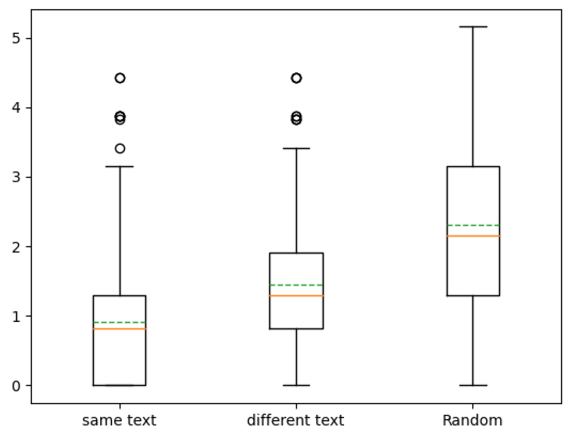
• There are two different versions, in the first one, the sentence is the same in the reference and in the 2D space. In the second, they are not. You just need to select the red point that in your opinion has the closest expressiveness.
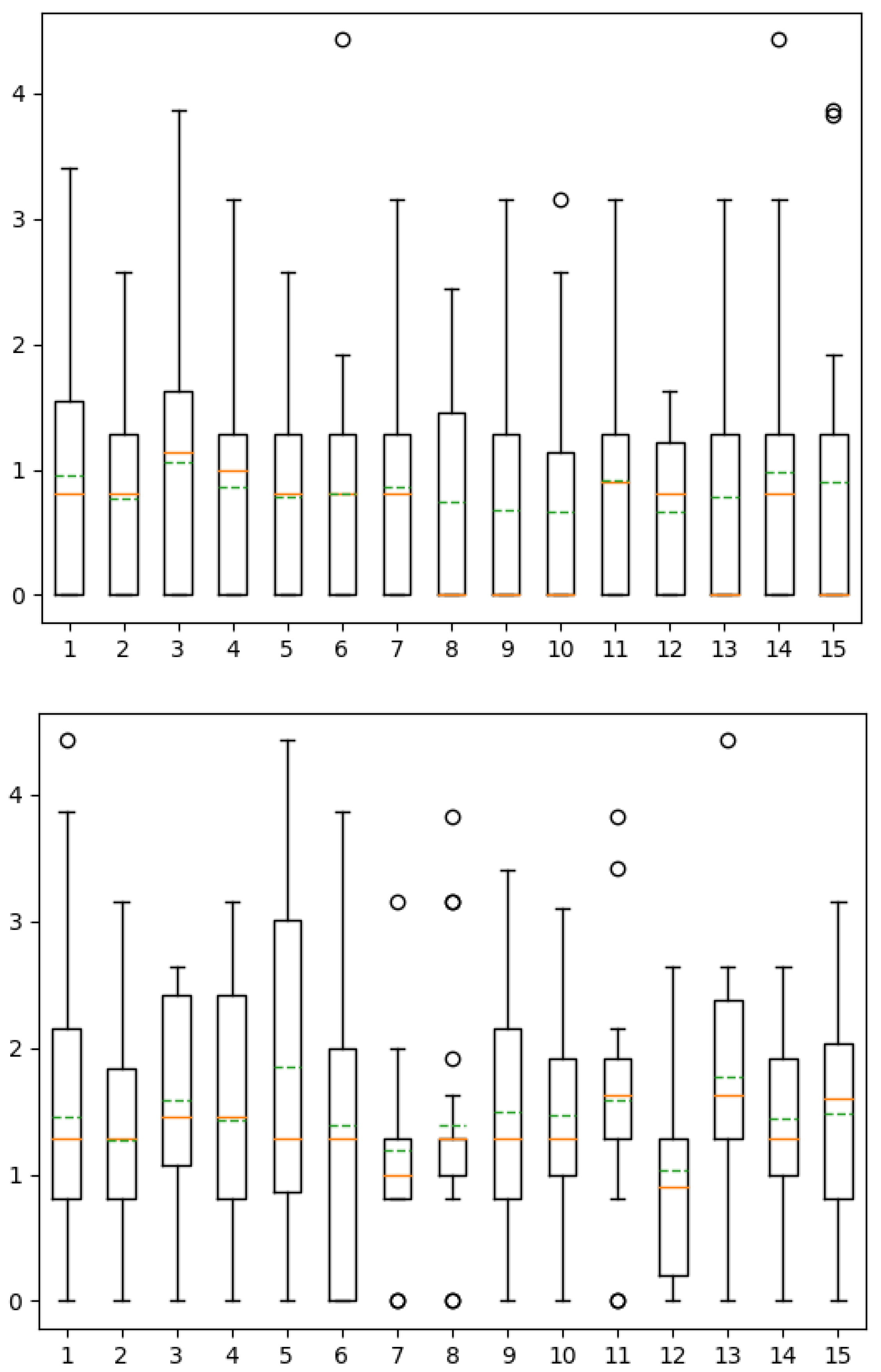
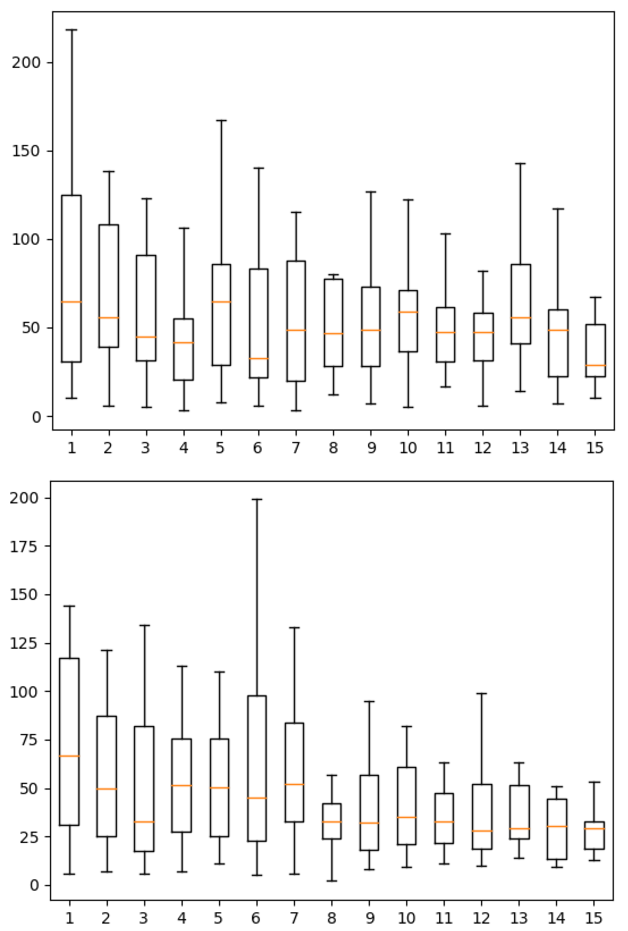
• It would be great if you could do this for a set of 15 samples in each level. You can see your evolution on the page.

A total of 25 and 26 people participated in variants 1 and 2 of the experiment, respectively. We collected a total of 488 and 326 answers, respectively.

6.2. Evaluation

6.2.1. Controllability Score

To quantify how well the participants were able to produce a desired expressiveness, we computed an average euclidean distance between the selected point and its true location.

Inspired by the omnipresent 5-point scales in the field of perceptual assessment, such as MOS tests, we choose to discretize the 2D space in a five-by-five grid, as shown in Figure 5. Indeed, a continuous scale could be overwhelming for participants and leave them unsure about their decision. The unit of distance is that between a red point and its neighbor along the horizontal axis.

We use a random baseline to assess the level of a non-controllability of the system in terms of expressiveness. In other words, if a participant is not able to distinguish the differences in expressiveness of different samples, we assume that he would not be able to select the correct location of the expressiveness of the reference and would answer randomly.

6.2.2. Results and Discussion

Figure 6 shows the distributions of the distances between participant answers and true location of references in the 2D space. The two variants (with same text and different text) are on the left and the random baseline is on the right. The average distances with 95% confidence intervals of the three distributions are, respectively: $0.908\pm 0.083$, $1.448\pm 0.103$, and $2.314\pm 0.007$.

The second version was considered much more difficult by participants. For the first task, it is possible to listen to every detail of the intonation to detect if the sentence is the same. That strategy is not possible for the second one in which only an abstract notion of expressiveness has to be imagined.

Furthermore, the speech rate is more difficult to compare between two different sentences than for the same sentence. Generally speaking, when there is not the same number of syllables, it is more difficult to compare the melody and the rhythm of the sentences (Figure 7).

The cues mentioned by participants include intonation, tonic accent, speech rate, and rhythm.

Figure 8 shows the distributions of the durations for participants to answer one question by index until the participants’ 15th answer. We can see in this figure that, over time, participants are progressively more constant in the duration and show a lower median duration. Outliers were discarded for plotting because they were too far from the distribution. The maximum is above 17,500 s. We believe these outliers are due to pauses taken by participants during the test. Furthermore, the means are influenced by these outliers and are therefore not plot in the figure.

A least square linear regression on the medians shows that it decreases with a slope of $-0.767$ s/task for the first variant and $-2.086$ s/task for the second. The two-sided p-values for the hypothesis test whose null hypothesis is that the slope is zero are, respectively, $0.21$ and $0.0004$. We can therefore reject the null hypothesis in the second case but not in the first.

Participants know more how to do it after several samples. They can guess where they have to search. They can establish a strategy as they understand how the space is structured. Therefore they feel like it is easier, and they can make a choice faster because they hesitate less.

However, the evolution of average scores do not seem to improve or decline over time. A least square linear regression on the average scores show slopes close to zero for both variant 1 and 2 (respectively $-0.005$ and $0.0001$ s/task). The two-sided p-value for a hypothesis test whose null hypothesis is that the slope is zero are, respectively, $0.496$ and $0.930$. It indicates strong evidence that the slope is zero; i.e., the evolution of average scores remains stable.

7. Summary and Conclusions

This paper presented a methodology for automatically building latent spaces related to expressiveness in speech data, for the purpose of controlling expressiveness in speech synthesis without referring to expert-based models of expressiveness. We then studied the relationships between such latent spaces and known audio features to obtain a sense of the impact of such audio features on the styles expressed. This analysis consisted in an approximation of audio features from embeddings by linear regression. The accuracy of approximations was then evaluated in terms of correlations with ground truth.

The gradient of these linear approximations were computed to extract the information from variations of audio features in speech. By visualizing these gradients along with the embeddings, we observed the trends of audio features in latent spaces.

A perceptual experiment was designed to evaluate the controllability of an Expressive TTS model based on these latent spaces. For that purpose, a set of reference utterances were synthesized with expressive control taken from discrete points in the 2D-reduced latent space. Test utterances were also synthesized with expressive control taken from a 5-by-5 grid on this 2D space. Participants were then asked to search this 2D grid for the test utterance corresponding to the expressiveness of a reference utterance. An average distance on the grid was computed and compared to a random baseline. Two variants of the task were presented to participants: in the first one, the same sentence was used for the reference and test utterances, while in the second they were different. Results show that the average distance is lower for the first task than for the second, and that they are both lower than the random baseline.

8. Perspectives

We presented a 2D interface in which we can explore a space of expressiveness. It could be interesting to investigate ways to control more vocal characteristics and independently when it is consistent and possible. Several types of controls could be investigated depending on the nature of the variables. For some variables, the control could consist of a set of choices, e.g., male/female or a list of speaker identities.

We also could imagine having two separate 2D spaces. One would be dedicated to a speaker identity, i.e., a space organizing voice timbres. Furthermore, the second would, e.g., have the 2D space of expressiveness presented in this paper. This kind of application needs frameworks able to disentangle speech characteristics and factorize information corresponding to different phenomena, such as phonetics, speaker characteristics, and expressiveness in the generated speech.

In the context of having more and more general systems, the research results of this paper that focus on English language could be adapted to obtain a system able to work with several languages. This could be considered as one more aspect of speech that needs to be factorized with others mentioned in the previous paragraph.

There are also possibilities of controlling the evolution of speech characteristics inside a sentence, referred to as fine-grained control that could be interesting to investigate. Currently, this aspect is mostly present in prosody transfer tasks and is not subject to a control involving a human choosing what intonation, tonic accent or voice quality he would like to hear at different parts of a sentence. The difficulty would be to select the relevant characteristics that a sound designer would want to control and design an intuitive interface to control them.

The different possibilities in this area would be interesting for, e.g., video games producer for the development of virtual characters with expressive voices, for animation movies, synthetic audiobooks, or in the advertisement sector.

References

- Burkhardt, F.; Campbell, N. Emotional speech synthesis. In The Oxford Handbook of Affective Computing; Oxford University Press: New York, NY, USA, 2014; p. 286. [Google Scholar]
- Tits, N. A Methodology for Controlling the Emotional Expressiveness in Synthetic Speech—A Deep Learning approach. In Proceedings of the 2019 8th International Conference on Affective Computing and Intelligent Interaction Workshops and Demos (ACIIW), Cambridge, UK, 3–6 September 2019; pp. 1–5. [Google Scholar] [CrossRef] [Green Version]
- Tits, N.; Haddad, K.E.; Dutoit, T. ICE-Talk 2: Interface for Controllable Expressive TTS with perceptual assessment tool. Softw. Impacts 2021, 8, 100055. [Google Scholar] [CrossRef]
- Ito, K. The LJ Speech Dataset. 2017. Available online: https://keithito.com/LJ-Speech-Dataset/ (accessed on 29 August 2021).
- Tits, N.; El Haddad, K.; Dutoit, T. The Theory behind Controllable Expressive Speech Synthesis: A Cross-Disciplinary Approach. In Human-Computer Interaction; IntechOpen: London, UK, 2019. [Google Scholar] [CrossRef] [Green Version]
- Watts, O.; Henter, G.E.; Merritt, T.; Wu, Z.; King, S. From HMMs to DNNs: Where do the improvements come from? In Proceedings of the 2016 IEEE International Conference on Acoustics, Speech and Signal Processing (ICASSP), Shanghai, China, 20–25 March 2016; pp. 5505–5509. [Google Scholar]
- Zen, H.; Tokuda, K.; Black, A.W. Statistical parametric speech synthesis. Speech Commun. 2009, 51, 1039–1064. [Google Scholar] [CrossRef]
- Zen, H.; Senior, A.; Schuster, M. Statistical parametric speech synthesis using deep neural networks. In Proceedings of the 2013 IEEE International Conference on Acoustics, Speech and Signal Processing (ICASSP), Vancouver, BC, Canada, 26–31 May 2013; pp. 7962–7966. [Google Scholar]
- van den Oord, A.; Dieleman, S.; Zen, H.; Simonyan, K.; Vinyals, O.; Graves, A.; Kalchbrenner, N.; Senior, A.W.; Kavukcuoglu, K. WaveNet: A Generative Model for Raw Audio. arXiv 2016, arXiv:1609.03499. [Google Scholar]
- Wang, Y.; Skerry-Ryan, R.J.; Stanton, D.; Wu, Y.; Weiss, R.J.; Jaitly, N.; Yang, Z.; Xiao, Y.; Chen, Z.; Bengio, S.; et al. Tacotron: Towards End-to-End Speech Synthesis. In Proceedings of the Interspeech 2017, Stockholm, Sweden, 20–24 August 2017. [Google Scholar]
- Skerry-Ryan, R.; Battenberg, E.; Xiao, Y.; Wang, Y.; Stanton, D.; Shor, J.; Weiss, R.; Clark, R.; Saurous, R.A. Towards End-to-End Prosody Transfer for Expressive Speech Synthesis with Tacotron. In Proceedings of the International Conference on Machine Learning 2018, Stockholm, Sweden, 10–15 July 2018; pp. 4693–4702. [Google Scholar]
- Klimkov, V.; Ronanki, S.; Rohnke, J.; Drugman, T. Fine-Grained Robust Prosody Transfer for Single-Speaker Neural Text-To-Speech. In Proceedings of the Interspeech 2019, Graz, Austria, 15–19 September 2019; pp. 4440–4444. [Google Scholar] [CrossRef] [Green Version]
- Karlapati, S.; Moinet, A.; Joly, A.; Klimkov, V.; Sáez-Trigueros, D.; Drugman, T. CopyCat: Many-to-Many Fine-Grained Prosody Transfer for Neural Text-to-Speech. In Proceedings of the Interspeech 2020, Shanghai, China, 25–29 October 2020; pp. 4387–4391. [Google Scholar] [CrossRef]
- Akuzawa, K.; Iwasawa, Y.; Matsuo, Y. Expressive Speech Synthesis via Modeling Expressions with Variational Autoencoder. In Proceedings of the Interspeech 2018, Hyderabad, India, 2–6 September 2018; pp. 3067–3071. [Google Scholar] [CrossRef] [Green Version]
- Taigman, Y.; Wolf, L.; Polyak, A.; Nachmani, E. Voiceloop: Voice fitting and synthesis via a phonological loop. arXiv 2017, arXiv:1707.06588. [Google Scholar]
- Hsu, W.N.; Zhang, Y.; Weiss, R.J.; Zen, H.; Wu, Y.; Wang, Y.; Cao, Y.; Jia, Y.; Chen, Z.; Shen, J.; et al. Hierarchical Generative Modeling for Controllable Speech Synthesis. arXiv 2018, arXiv:1810.07217. [Google Scholar]
- Henter, G.E.; Lorenzo-Trueba, J.; Wang, X.; Yamagishi, J. Deep Encoder-Decoder Models for Unsupervised Learning of Controllable Speech Synthesis. arXiv 2018, arXiv:1807.11470. [Google Scholar]
- Wang, Y.; Stanton, D.; Zhang, Y.; Ryan, R.S.; Battenberg, E.; Shor, J.; Xiao, Y.; Jia, Y.; Ren, F.; Saurous, R.A. Style Tokens: Unsupervised Style Modeling, Control and Transfer in End-to-End Speech Synthesis. In Proceedings of the International Conference on Machine Learning 2018, Stockholm, Sweden, 10–15 July 2018; pp. 5180–5189. [Google Scholar]
- Shechtman, S.; Sorin, A. Sequence to sequence neural speech synthesis with prosody modification capabilities. arXiv 2019, arXiv:1909.10302. [Google Scholar]
- Raitio, T.; Rasipuram, R.; Castellani, D. Controllable neural text-to-speech synthesis using intuitive prosodic features. arXiv 2020, arXiv:2009.06775. [Google Scholar]
- Tits, N.; El Haddad, K.; Dutoit, T. Neural Speech Synthesis with Style Intensity Interpolation: A Perceptual Analysis. In Companion of the 2020 ACM/IEEE International Conference on Human-Robot Interaction; Association for Computing Machinery: New York, NY, USA, 2020; pp. 485–487. [Google Scholar] [CrossRef] [Green Version]
- Tachibana, H.; Uenoyama, K.; Aihara, S. Efficiently trainable text-to-speech system based on deep convolutional networks with guided attention. In Proceedings of the 2018 IEEE International Conference on Acoustics, Speech and Signal Processing (ICASSP), Calgary, AB, Canada, 15–20 April 2018; pp. 4784–4788. [Google Scholar]
- Tits, N.; Wang, F.; Haddad, K.E.; Pagel, V.; Dutoit, T. Visualization and Interpretation of Latent Spaces for Controlling Expressive Speech Synthesis through Audio Analysis. In Proceedings of the Interspeech 2019, Graz, Austria, 15–19 September 2019; pp. 4475–4479. [Google Scholar] [CrossRef] [Green Version]
- Eyben, F.; Scherer, K.R.; Schuller, B.W.; Sundberg, J.; André, E.; Busso, C.; Devillers, L.Y.; Epps, J.; Laukka, P.; Narayanan, S.S.; et al. The Geneva minimalistic acoustic parameter set (GeMAPS) for voice research and affective computing. IEEE Trans. Affect. Comput. 2016, 7, 190–202. [Google Scholar] [CrossRef] [Green Version]
- Kubichek, R. Mel-cepstral distance measure for objective speech quality assessment. In Proceedings of the IEEE Pacific Rim Conference on Communications Computers and Signal Processing, Victoria, BC, Canada, 19–21 May 1993; Volume 1, pp. 125–128. [Google Scholar]
- Nakatani, T.; Amano, S.; Irino, T.; Ishizuka, K.; Kondo, T. A method for fundamental frequency estimation and voicing decision: Application to infant utterances recorded in real acoustical environments. Speech Commun. 2008, 50, 203–214. [Google Scholar] [CrossRef]