Abstract
One of the main limitations of the typical hidden Markov model (HMM) implementation for gene structure identification is that a single structure is identified on a given sequence of genomic data—i.e., identification of overlapping structure is not directly possible, and certainly not possible within the confines of the optimal Viterbi path evaluation. This is a huge limitation given that we now know that significant portions of eukaryotic genomes, particularly mammalian genomes, are alternatively spliced, and, thus, have overlapping structure in the sense of the mRNA transcripts that result. Using the general meta-state HMM approach developed in prior work, however, more than one ‘track’ of annotation can be accommodated, thereby allowing a direct implementation of an alternative-splice gene-structure identifier. In this paper we examine the representation of alternative splicing annotation in the multi-track context, and show that the proliferation on states is manageable, and has sufficient statistical support on the genomes examined (human, mouse, worm, and fly) that a full alt-splice meta-state HMM gene finder can be implemented with sufficient statistical support. In the process of performing the alternative splicing analysis on alt-splice event counts we expected to see an increase in alternative splicing complexity as the organism becomes more complex, and this is seen with the percentage of genes with alt-splice variants increasing from worm to fly to the mammalian genomes (mouse and human). Of particular note is an increase in alternative splicing variants at the start and end of coding with the more complex organisms studied (mouse and human), indicating rapid new first and last exon recruitment that is possibly spliceosome mediated. This suggests that spliceosome-mediated refinements (acceleration) of gene structure variation and selection, with increasing levels of sophistication, has occurred in eukaryotes and in mammals especially.
1. Introduction
Computational gene-finding work began to make significant advances in the 1980s [1,2,3], especially upon introduction of hidden Markov models (HMMs), both in statistics intrinsic to the genome under study (ab initio gene-finding) [1,2,3], and in analysis involving statistics extrinsic to the genome using sequence similarity/alignments methods (e.g., homology or expressed sequence tag, EST, matching with finite state automata, ‘FSAs’) [4]. Alignment, of query sequences to a known sequence in a database is typically done using BLAST [5] (which involves a hybrid HMM/FSA method). BLAST can also be used for gene finding alone, where homology-based programs can be used to identify new genes by aligning a query sequence with a known gene or genes [4]. More complex gene-finders that use extrinsic statistical information for the genome, along with intrinsic genomic information (from statistical properties of the genomic sequence data alone), have also been implemented [6]. The main drawback of homology-based approaches is that they cannot find new genes if they are significantly different from the known gene sequences in the known-gene databases, as discussed in [1], and explored in [7]. This is a significant limitation to purely homology-based approaches since approximately half of the genes in a particular eukaryotic genome appear to be novel to that genome (such as for C. elegans). This also appears to be the case for human, where only about half of the proteins encoded in chromosome 22, for example, are found to be similar to previously known proteins. In [8], the author describes application of a highly successful gene-finder known at that time (ca. 2004) to gene-finding in novel genomes. From that study it is clear that gene-prediction has species-specific statistical properties, i.e., an ab initio component must operate for any gene-finder to succeed at identifying genes and genomic structures novel to that organism [8].
Starting around 2000 there was a movement towards consolidation of the intrinsic and extrinsic approaches [7,9], as described in a 2002 review [9] and a 2006 review [10]. At that time there were fundamental modeling limitations with the standard HMM implementation. So much so that in the 2006 review it was claimed that “improved modeling efforts at the hidden Markov model level are of relatively little value”. In the [11,12,13] publications that appeared in 2010 and 2011, however, generalized HMMs (gHMMs) with significantly improved modeling capabilities were shown that could be implemented very efficiently, sometimes with time-complexity comparable to the standard HMM. What resulted was a clear improvement in HMM capabilities in gene-finding [11,12,13], and in application to stochastic sequential data in general. Also beginning around 2000 was specialization to sensor development [14,15,16,17,18,19,20] to help supplement the HMM-based structure discovery process. There were sensors for transcription start site prediction [6], transcription initiation sites and polyadenylation signals [21], splice-site recognition [22,23], and identification of 3’ ends of exons by EST analysis [24], to list just a few examples.
Since 2000, there has also been rapid growth in the development of motif-discovery algorithms—in parallel with the aforementioned sensor specialization. Many of these motif-discovery algorithms can be used to augment the HMM-based structure identification via motif-based validation of gene-structure regions indicated by the HMM. Using ‘zone dependent’ Markov modeling in gene-finding at high Markov order [12], it is possible to both effectively capture regulatory motifs by their anomalously high occurrence rate, and to absorb this into the overall HMM structure identification task [11,12]. In [11,12,25,26], many important transcription factor binding sites (TFBS’s), miRNA binding sites, promoters, and other regulatory motifs can be identified by their position relative to the start and stop of coding (and other non-self-transitions identified by the HMM’s optimal Viterbi-path parsing). In [25] it is shown that the motif finding effort is greatly enhanced by referencing to nearby gene-structure and identifying local regions for focused motif searches. Not surprisingly, if separate statistical profiling is performed on the regions just outside the translation region (cis and trans), then gene-finding is improved [13,25]. Motif discovery can be focused on the cis-regulatory regions for TFBS discovery and on the trans-regulatory regions for miRNA binding site discovery, and if linked with the HMM discovery, the motif-discovery and gene-discovery efforts are simultaneously strengthened. Using an intrinsic HMM formulation as a foundation, with extrinsic statistical information from motif discovery and signal-sensor augmentations, one then arrives at a unified and powerful intrinsic/extrinsic gene and motif discovery platform. This capability is enhanced further if zone-dependent emissions are employed [12] or via reference to HMMD improvements as indicated in [12,13,27]. The HMM formulation with HMMD augmentation (technically a form of hidden semi-Markov model) also provides a local state-path optimization that can directly, locally in the dynamic programming table construction, incorporate extrinsic statistics (side-information) into the Viterbi optimization (as described in [13]). The ‘scaffolding’ provided by the HMMD parsing (via the Viterbi path derivation) defines regions where zone-dependent statistics and zone-restricted motif-discovery can be applied. With zone-restricted motif discovery, gap and hash interpolated Markov model’s [28,29] become powerful tools for motif discovery in a restricted region [21,29,30,31,32,33]. The approach we describe in [11,12,13], seeks to unify the above approaches within a powerful new HMM-based structure-modeling architecture.
The shortcomings of the HMM due to algorithmic definitions, such as lack of state-duration modeling, are readily apparent (with fixes as described in [12,13,27]). The shortcomings of the HMM due to choice of model definition and related implementation, are more subtle. In an HMM implementation the number of look-ups to a particular emission or transition probability table will show how that table’s anomalous statistics influence the overall computation (where the count on use of a particular component in the table is precisely what provides an estimation in the HMM Baum–Welch algorithm). Standard HMM’s lead to a model that strongly de-emphasizes (with low table usage) the anomalous statistics known to exist around non-self-transitions, and restricts to transition probabilities that are not sequence dependent. In [11] it is shown that use of transition probabilities that are sequence dependent, via use of a constrained set of ‘meta-states’, is possible with comparable computational complexity to the standard HMM. There is, thus, a ‘model primitive’ shortcoming underlying the standard HMM implementation that is resolved in the meta-state HMM description [11].
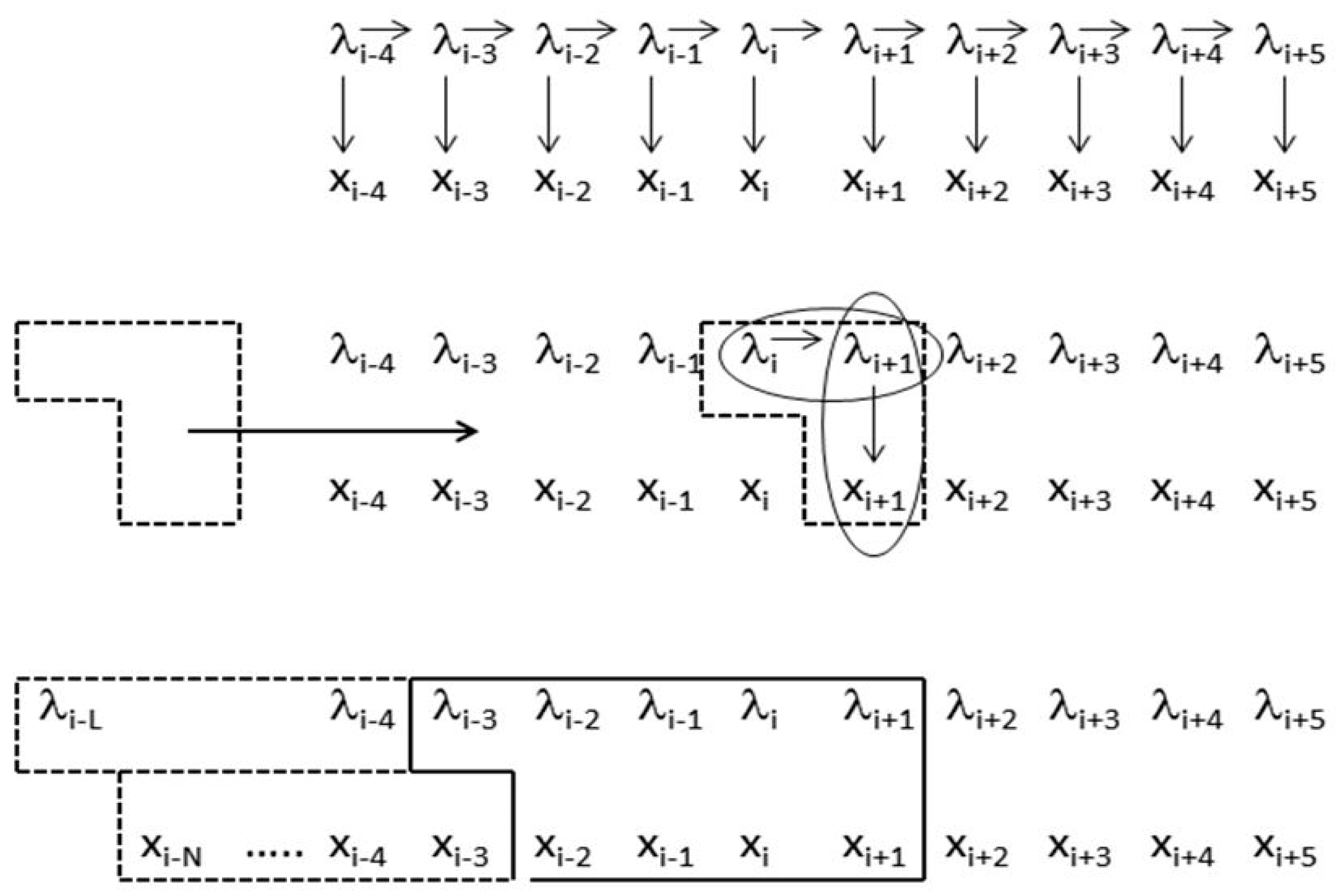
The generalized-clique, ‘meta-state’, hidden Markov model introduced in [11] has been applied to the analysis of the genomic structure of C. elegans (a genome-data intrinsic approach, e.g., not using EST or homology information). The meta-state HMM generalizes from primitive states to windows of adjacent primitive states (e.g., “footprint states”), and does so by only allowing one coding-to-noncoding, or noncoding-to-coding, transition in the footprint state. A comparison between the clique structure of the standard HMM and the meta-state HMM is shown in Figure 1, with comparative performance results for the meta-state HMM and standard HMMs shown in application to C. elegans (worm) shown in Supplementary Section 1 (Tables S1 and S2). The constraint to have no more than a single ‘non-self’ transition in a footprint is equivalent to a minimum length constraint on exons, introns, and ‘junk’. The linear growth in footprint states with this constraint (shown in [11] and described in Supplementary Section 2) is critical for practical use of the larger footprint size models.
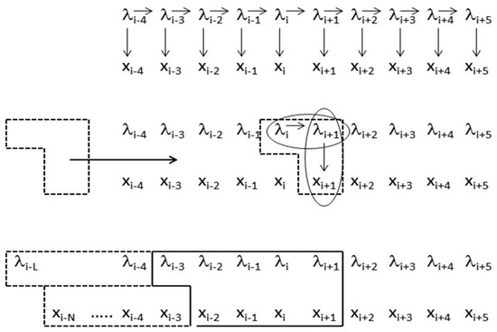
Figure 1.
Comparison of standard hidden Markov model (HMM) and the clique-generalized meta-state HMM. The upper graphical model is for the standard HMM and shows the ‘emission’ observation sequence xi, and the associated hidden label sequence λi, and the arrows denote the conditional probability approximations used in the model (for the transition and emission probabilities). Focusing at the level of the core joint-probability construct at instant ‘i’ in the middle graph, the standard HMM is a subset of the joint probability construct P(λi, λi+1, xi+1). The generalized-clique HMM is shown in the graphical model at the bottom for one particular clique generalization. The model can be exact on emission positionally, then extend via zone dependence and use of generalized HMM (gIMM) interpolation. The model can be exact to higher order in state, and using an HMMD generalization [12] also extends modeling to have HMM with duration modeling. When doing the latter, zone-dependent and position dependent modeling can be incorporated via reference to the duration in the model, and can be directly incorporated into a generalized Viterbi algorithm (and other generalized HMM algorithms), as well as any other side-information of interest [13]. Reprinted with permission [11].
Using the general meta-state HMM approach, however, more than one ‘track’ of annotation can be accommodated, thereby allowing a direct implementation of an alternative-splice gene-structure identifier. There is still the necessity, however, for there to be sufficient statistical support (e.g., samples) on the non-self-transitions to have a reliable profile HMM developed (e.g., establish the bare-bones HMM sensors). This can only succeed, practically speaking, if the multi-track annotation describing the alternative splicing can be represented with a manageable number of multi-track transition states, where the intrinsic genomic statistics on these multi-tack states has sufficient support to properly model the proliferation in meta-states that results.
In this paper we examine the representation of alternative splicing annotation in the multi-track context, and show that the proliferation on states is manageable, and has sufficient statistical support on the Genbank annotated genomes examined (human, mouse, worm, fly) that a full alt-splice meta-state HMM gene finder can be implemented using an analysis only based on the intrinsic statistical information of the genome studied (the actual implementation will be done in a separate paper). The four organisms selected in this study are all animals, thus our focus is on eukaryotes that are animals and not plants or protists (or single-celled anything). Plants and protists will be the focus of later studies.
2. Background
A brief background is given for the standard first order HMM, followed by background on its meta-state HMM generalization (where the derivation of associated generalized Viterbi and Baum–Welch algorithms is given in [11]). Background information is then given for the HMM states and transitions, and their representations, that are relevant in the context of alt-splice gene structure identification.
2.1. The Standard 1st Order HMM
We define the 1st order HMM as consisting of the following:
- A hidden state alphabet, Λ, with “Prior” Probabilities P(λ) for all λ Λ, and “Transition” Probabilities P(λ2|λ1) for all λ1 λ2 Λ—where the standard transition probability is denoted akl = P(λn = l|λn−1 = k) for a 1st order Markov model on states with homogenous stationary statistics (i.e., no dependence on position ‘n’).
- An observable alphabet, B, with “Emission” Probabilities P(b|λ) for all λ Λ b B—where the standard emission probability is ek(b) = P(bn = b|λn = k), i.e., a 0th order Markov model on bases with homogenous stationary statistics.
Given the above, there are three classes of problems that the HMM can be used to solve [34,35]:
- Evaluation—Determine the probability of occurrence of the observed sequence.
- Learning (Baum–Welch)—Determine the most likely emission and transition probabilities for a given set of observational data.
- Decoding (Viterbi)—Determine the most probable sequence of states emitting the observed sequence.
Here we focus only on the 3rd problem, the Viterbi decoding problem. The probability of a sequence of observables B = b0, b1, …, bn−1 being emitted by the sequence of hidden states Λ = λ0, λ1, …, λn–1 is solved by using P(B, Λ) = P(B|Λ)·P(Λ) in the standard factorization, where the two terms in the factorization are described as the observation model and the state model, respectively. In the 1st order HMM, the state model has the 1st order Markov property and the observation model is such that the current observation, bn, depends only on the current state, λn:
P(B|Λ)·P(Λ) = P(b0|λ0) P(b1|λ1)…P(bn–1|λn–1) × P(λ0)P(λ1|λ0)P(λ2|λ0, λ1)…P(λn–1|λ0…λn−2)
With first order Markov assumption in the state-model this becomes:
P(B|Λ) P(Λ) = P(b0|λ0) P(b1|λ1)…P(bn–1|λn–1) × P(λ0)P(λ1|λ0)P(λ2|λ1)…P(λn–1|λn–2)
In the Viterbi algorithm, a recursive variable is defined (following the notation in [34]): vk(n) = “the most probable path ending in state ‘k’ with observation ‘bn’”. The recursive definition of vk(n) is then: vl(n + 1) = el(bn+1) maxk [vk(n) akl]. From which the optimal path information is recovered according to the (recursive) trace-back:
Λ* = argmaxΛ P(B, Λ) = (λ*0, …, λ*n−1)
λ*n|λ*n+1 = 1 = argmaxk [vk(n) akl], and where λ*L–1 = argmaxk [vk(L – 1)], for length L sequence.
2.2. The Meta-State HMM
The generalized clique HMM begins by enlarging the primitive hidden states associated with individual base labeling (as exon, intron, or junk) to substrings of primitive hidden states or footprint states (details on the definitions of the base-label states and footprint states are in Section 2.3 and Supplementary Section 2). In what follows, the transitions between primitive hidden states for coding {e} and non-coding {i, j}, {ei, ie, je, ej}, are referred to as ‘eij-transitions’, and the self-transitions, {ee, ii, jj}, are referred to as ‘xx-transitions’. The emissions are likewise expanded to higher order in the fundamental joint probability that is the basis of the generalized-clique, or ‘meta-State’, HMM. In [11] we consider application to eukaryotic gene finding and show how a meta-state HMM improves the strength of eij-transition contributions to gene-structure identification. It is found that the meta-state eij-transition modeling can effectively ‘recapture’ the exon and intron heavy tail distribution modeling capability as well as manage the exon-start ‘needle-in-the-haystack’ problem [11].
The meta-state, clique-generalized, HMM entails a clique-level factorization rather than the standard HMM factorization (that describes the state transitions with no dependence on local sequence information). This is described in the general formalism to follow, where specific implementations are given for application to eukaryotic gene structure identification.
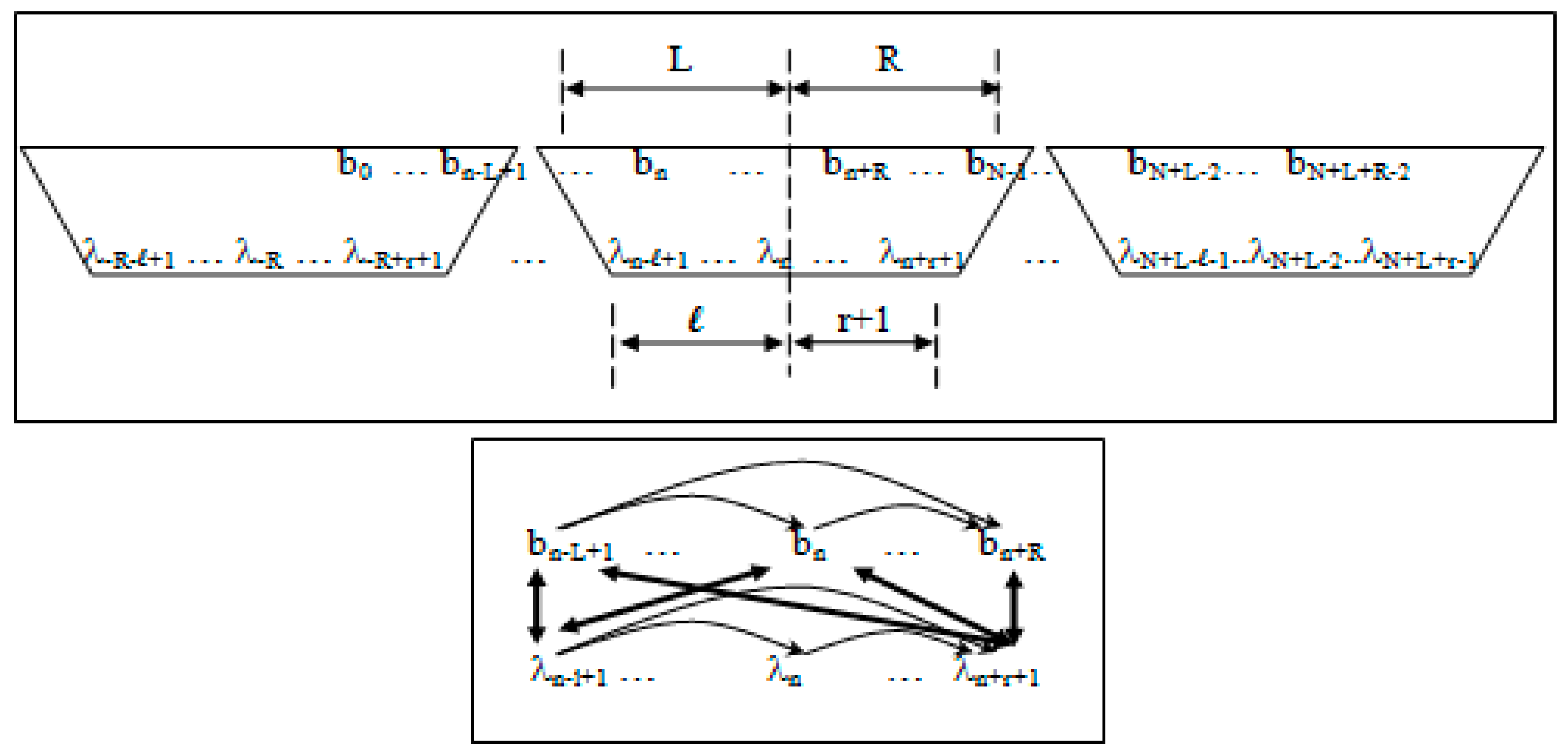
Observation and state dependencies in the generalized-clique HMM (see Figure 2) are parameterized according to the following:
- 1)
- Non-negative integers L and R denoting left and right maximum extents of a substring, wn, (with suitable truncation at the data boundaries, b0 and bN−1) are associated with the primitive observation, bn , in the following way:
- wn = bn−L+1, …, bn, …, bn+R
- n = bn−L+1, …, bn, …, bn+R−1
- 2)
- Non-negative integers l and r are used to denote the left and right extents of the extended (footprint) states, f. Here, we show the relationships among the primitive states λ, dimer states s, and footprint states f:
- δn = λnλn+1 (dimer state, length in λ’s = 2)
- fn = δn−l+1, …, δn+r ≅ λn−l+1, …, λn, …, λn+r+1 (footprint state, length in δ’s = l + r)
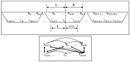
Figure 2.
Top Panel. Sliding-window association (clique) of observations and hidden states in the meta-state hidden Markov model, where the clique-generalized HMM algorithm describes a left-to-right traversal (as is typical) of the HMM graphical model with the specified clique window. The first observation, b0, is included at the leading edge of the clique overlap at the HMM’s left boundary. For the last clique’s window overlap we choose the trailing edge to include the last observation bN–1. Bottom Panel. Graphical model of the clique-generalized HMM, where the interconnectedness on full joint dependencies is only partly drawn. Reprinted with permission [11].
As in the 1st order HMM, the n-th base observation bn is aligned with the n-th hidden state λn. Given the above, the clique-factorized HMM is as follows [11]:
The critical ratio of probabilities in the […] term above retains the Martingale sequence properties on the generalized Viterbi path, as with the standard HMM/Viterbi implementation, and all of the elegant convergence and limit properties of Martingales are thereby inherited via the backward martingale convergence theorem (as discussed in [36]). The sliding-window clique overlap (see Figure 1) is much more significant than with the standard HMM, giving rise to many more table look-ups on eij-transition tables.
A generalization to the Viterbi algorithm can now be directly implemented, using the above form, to establish an efficient dynamic programming table construction. Generalized expressions for the Baum-Welch algorithm are also possible. For further details on the generalized Viterbi and Baum-Welch algorithms for the meta-state HMM see [11,36] (and see Supplementary Tables S1 and S2 for some performance results).
2.3. HMM States and Transitions for Gene-Structure Identification
The codon structure in exons is directly revealed in a mutual information analysis of gapped base statistical linkages as shown in [28]. The partitioning of exon sequence into 3-base subsequences is known as the codon framing, where a gene’s coding length must be a multiple of 3 bases. The term frame position is used to denote one of the 3 possible positions—0, 1, or 2 by our convention—relative to the start of a codon. Introns may interrupt coding sequence after any frame position. In other words, introns can split the codon framing either at a codon boundary or one of the internal codon positions. To show this, denote the primitive states of the individual bases, described as exon, intron, or junk, by:
- Exon states = {e0, e1, e2}, where frame label is ‘real’, i.e., there are three emission tables;
- Intron states = {i0, i1, i2}, where frame label is a convenient implementation artifact (so one em table);
- Junk state = {j}, the non-coding (non-exonic) nucleotides in the intergenic regions, while the non-coding nucleotides in the intragenic regions are the aforementioned introns.
While ‘emitting’ the base sequence observed, the ‘real’ exon framing subscript ‘cycles’ over states corresponding to the frame position as expected, while the intron framing info stays the same and ‘transmits’ framing information thereby to the end of the intronic region (purely for the convenience in the HMM implementation). We thus have three possible intron ‘framings’ indicated in the following state strings (with exon framing shown cycling):
- jj...je0e1e2…e0i0i0…i0e1…e0e1e2jj…j (intron follows exon base with frame 0)
- jj...je0e1e2…e1i1i1…i1e2…e0e1e2jj…j (intron follows exon base with frame 1)
- jj...je0e1e2…e2i2i2…i2e0…e0e1e2jj…j (intron follows exon base with frame 2)
Using the base-level state labeling, consider the ‘toy’ gene shown in Figure 3 that has only two exons. The label information is shown consistent with this, and an ‘arrow’ notation is introduced in the figure to show how the arrow demarks the boundary of the intragenic region that will be used in the figures to follow.

Figure 3.
The standard forward-read Gene Predictor with five state labels: j, i, 0, 1, 2; and 13 state transitions: jj, j0, 2j, 01, 12, 20, 0i, 1i, 2i, i0, i1, i2, ii. The arrow covers the extent of the exon bounded region.
Although there is no notion of framing among introns, for convenience we associate framing with the intron for use in code implementation, as indicated in Figure 3, as a tracking device in order to ensure that the frame of the following intron-to-exon transition is constrained appropriately.
In [11], the 13 state transitions are not only extended to 15 to incorporate the above frame-tracking across introns, but further extended to 17 states to incorporate stop codon recognition/validation directly into the end-of-coding transition. The 17 two-label (dimer) forward transitions are: {jj, je0, e0e1, e1e2, e2e0, e0i0, e1i1, e2i2, i0i0, i1i1, i2i2, i0e1, i1e2, i2e0, e2j_TAA, e2j_TAG, e2j_TGA}. See Supplementary Section 2 for details on the 33-state model for the forward and reverse encoding together, to be described next.
There is further complexity in that the encodings for proteins can be found in both directions along the duplex DNA strand, where the forward and reverse encodings are found to be present in approximately equal numbers. Furthermore, the differences in the base statistics in the forward and reverse gene encodings are sufficiently negligible (or disjoint) that their counts can simply be merged in the modeling (data not shown). To see the application, consider using the above 17 transition model on dsDNA genomic data, a genome would then be analyzed by doing two passes on the genomic data reference strand provided, a forward pass and a reverse pass (see Figure 4).

Figure 4.
The standard two-pass gene predictor. A forward pass is used to catch forward reads, followed by a reverse complement pass to catch reverse reads.
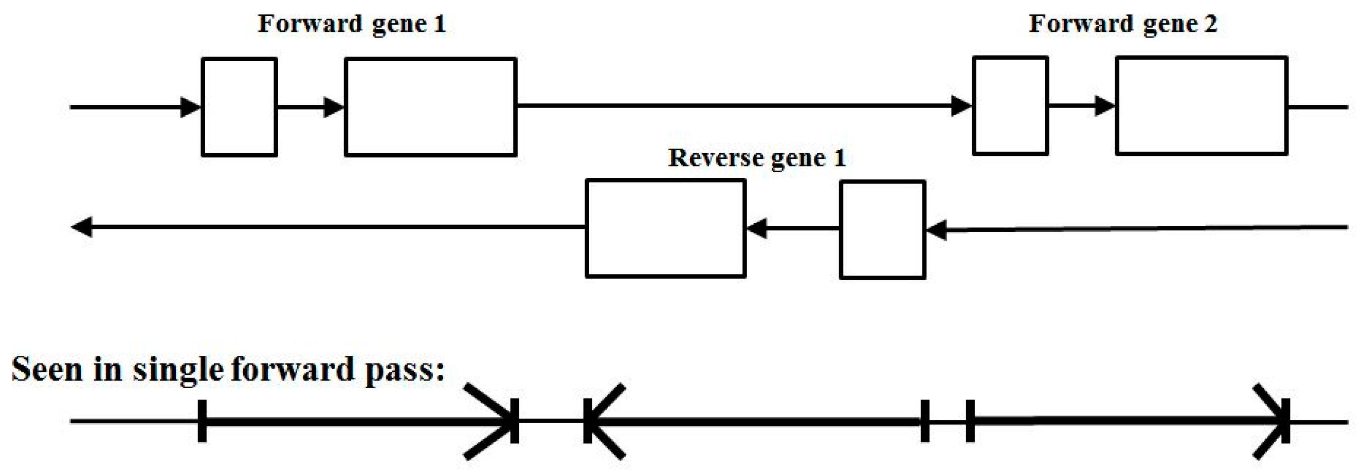
The problem with the decoupling of parsing on forward reads and reverse reads is that a forward read in a reverse coding region can encounter non-standard base statistics for ‘non-coding’ (since it’s the statistics of a reverse coding region), which can lead to error (see Figure 5).

Figure 5.
The problem with the standard two-pass gene predictor. Confusion can result in the forward pass across reverse read regions, as shown, that can obscure the true start of other, valid, forward reads.
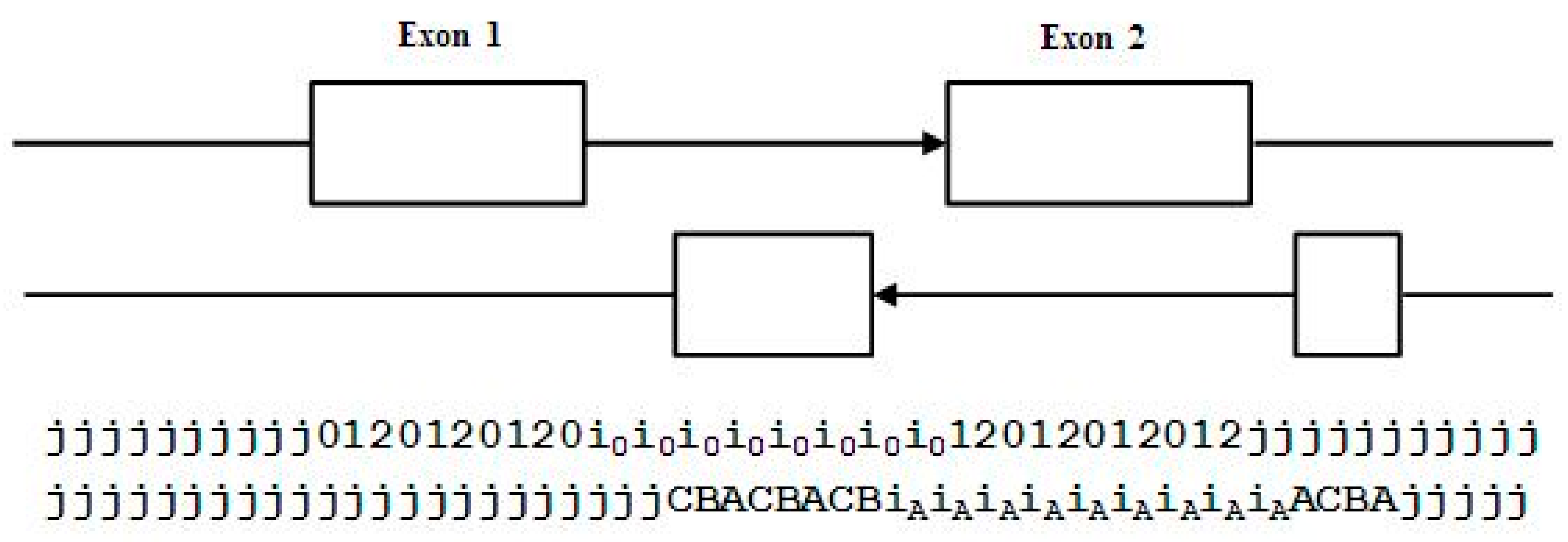
One possible solution to this, for the case where the forward and reverse gene encodings do not overlap is to capture both in a single pass involving state transitions describing both forward transitions and reverse transitions. There are nine states: j, i, I, 0, 1, 2, A, B, C; where A, B, C are the primitive labels on the reverse read coding bases, and I is for the reverse read intronic bases. The reverse-read codon is ‘CBA’. Accordingly, there are 25 state transitions: jj, j0, jC, 2j, Aj; 01, 12, 20, BA, CB, AC, 0i, 1i, 2i, i0, i1, i2, AI, BI, CI, IA, IB, IC, ii, II. In Figure 6 is shown two forward gene encodings on track 1 and one reverse encoding on track 2, where the forward and reverse encodings do not overlap. In the bottom part of Figure 6 is shown the forward and reverse (non-overlap) encodings on a single track using the arrow notation.
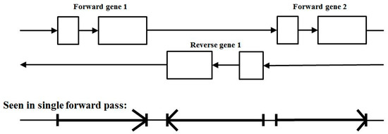
Figure 6.
The single-pass forward/reverse coding Gene Predictor with non-overlapping encoding. Top: the forward and reverse reads shown on two separate tracks. Bottom: the forward and reverse reads on a single forward-scan pass on an enlarged state and transition model (shown without refinement involving intron frame-pass and end-of-coding stop codon validation states).
Using a single-pass forward/reverse coding Gene Predictor, and using the previously mentioned refinements involving intron frame-pass and end-of-coding stop codon validation states, it is possible to work directly with both forward and reverse states. This type of HMM implementation has been done in [11] and results in a 33-element transition model (see Supplementary Section 2 for details). The 33 transitions can be taken as the states themselves (two-element meta-states, or ‘dimer’ states, or length 2 footprint states according to the terminology in [11] and in what follows).
In order to work directly with the above dimer states, or the footprint-state generalization, we need to generalize to a higher order HMM model (see Figure 1 and Figure 2, and performance results in Supplementary Section 1). The standard HMM has emissions that only depend on the current state (e.g., we have P(bn−1|λn−1) terms). A simple HMM with single-base state representation has poor performance in modeling the anomalous statistics in the transition regions between exon, intron, or junk regions without additional side-rules that break with a purely HMM implementation. If a transition ‘je0’ has occurred, for example, and we are looking at the base emission for the ‘e0’ state, we cannot account for the prior state with the simple P(bn−1|λn−1) conditional probabilities in the standard bare-bones HMM modeling, we minimally need P(bn−1|λn−2, λn−1), i.e., state modeling at the dimer-level or higher.
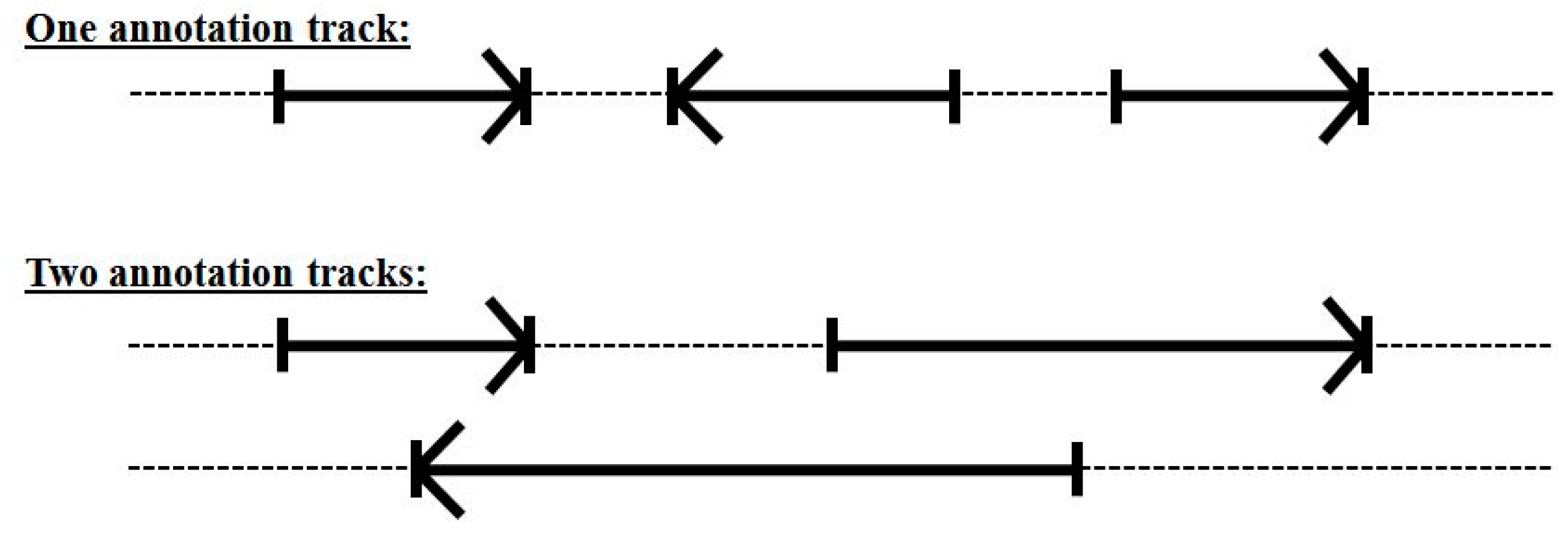
Even with the 33-state dimer footprint model above we still cannot handle overlapping encodings (alternative splicing or overlap with a reverse coding region). This was not a significant problem in the C. elegans genome analysis in [11], but when moving to human, where alternative-splicing is much more common (see Figure 7), the resulting HMM modeling will not perform as well as desired.
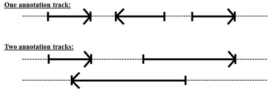
Figure 7.
Overlapping encoding requires more than one annotation track if using a single forward-pass gene-structure identifier.
Adding further complication is the fact that it is possible to have higher order overlaps requiring more tracks than two. Fortunately for the alt-splice gene prediction (AGP) modeling sought here this is much less common. Two tracks will be shown to not only provide an excellent statistical representation of the forward/reverse overlap encodings, but also alternative splicing alternate encodings where the same issue of occasional very highly alternatively splices section of genomes are known to exist (but are very rare, with typical alternative splicing giving one alternative). Thus, there is the use of ‘two tracks’ only in what follows, not three, or more.
In the genome annotations studied, forward and reverse transcripts often overlap, but often with their coding regions (exons) in the other transcript’s intronic regions (Figure 8). With the two-track annotation on states we can now introduce the notion of vertical (V) state labels (see Figure 8): … also denoted as a ‘jA’ V-state, and V-transitions: … also denoted as a ‘iiCB’ V-transition.
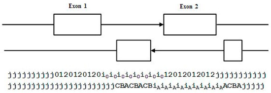
Figure 8.
Overlap of coding with reverse intronic regions, with individual base states shown below for the two tracks.
For alt-splice annotation representation with two tracks we have both reads in the same direction and the exon overlap with an intron region represents alternatively spliced transcripts where the exon has been, alternatively, spliced out (see Figure 9 and Supplementary Figure S1 for the two cases of exon/intron overlap, with the alt-spliced exon present on track 1, not track 2, in Figure 9, and vice versa in Supplementary Figure S1).

Figure 9.
Alt-splice overlap encoding with alternatively spliced exon present on track 1. We find V-state labels: , etc., and V-transitions: , compactly denoted ‘i1ii’, shown. Other 3-prime splice-site, intron-exon (ie), overlap with intron (ii) transitions include ‘i0ii’ and i2ii’. We also have V-transitions: , denoted ‘0iii’, for 5-prime splice-site, exon-intron (ei), overlap with intron (ii) transitions (other 5-prime ei overlap V-transitions include ‘1iii’ and 2iii’).
Less common than exon overlap with intron is partial exon overlap with intron/exon as shown in Supplementary Figure S2, where a 3-prime splice site overlap with alternative splice intron region is shown, denoted (3’|i). The total count on the 12 (3’|i) types will be shown for four genomes in the comparative analysis that follows (the genome data used is shown in Table 1). Also shown in Supplementary Figure S2 is a 5-prime splice site overlap with alternative splice intron region, denoted (5’|i). The total count on the 12 (5’|i) types will also be shown for four genomes in the comparative analysis that follows.

Table 1.
Genome versions.
3. Experimental Section—Methods
3.1. Genome Versions Used in Data Analysis (All from www.ensembl.org)
3.2. Pre-Partitioning Training Data for Massively Parallel/Distributed Solutions
Starting with the ensemble general transfer format (GTF) file of a particular organism, we run a script to identify the number of chromosomes, and any other discrete genomic elements present, according to the annotation listings, and these genomic elements are listed in a log file. The user is then allowed to edit this log file before further processing to delete out entries for chromosomes or other genomic elements on the list, and thereby exclude those deleted entries from the analysis that follows. If nothing is deleted (the file isn’t modified), then all of the chromosomes in the genome are used in the analysis, as was the case for the genomes examined here.
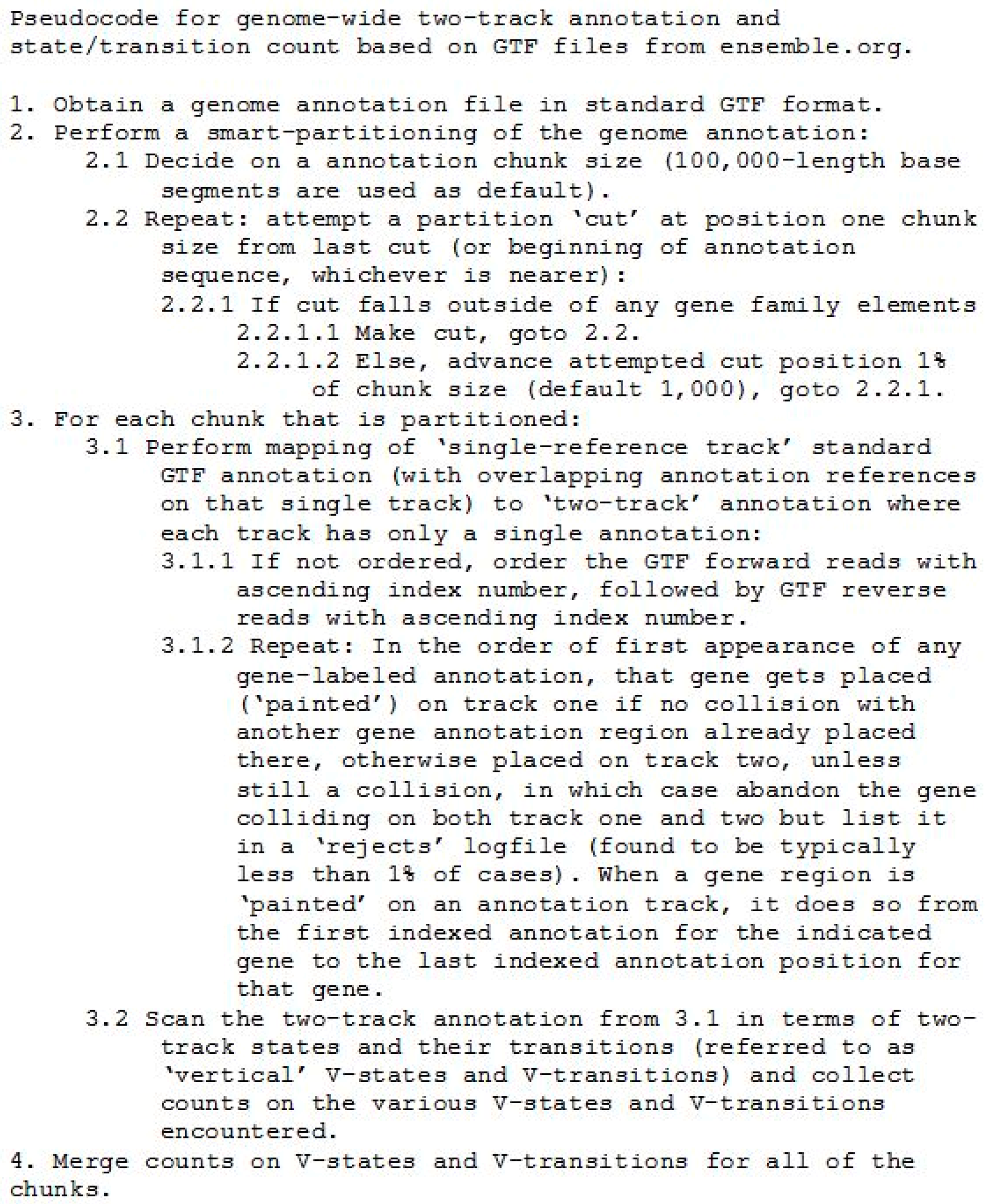
Each chromosome that is examined is modelled with a two-label-track annotation scheme that is derived from the (‘single-track’) GTF file annotations, where the two-track conversion scheme is described in Figure 10 and Figure 11. The general implementation of the HMM modelling software allows for arbitrarily many tracks, so three or more tracks could have been accommodated if necessary, but this turns out to not be the case for the genomes examined (fortunately, as there is then sufficient support from an ab initio analysis of the genomes examined for a two-track label scheme, but only barely for the rarest transition states, as will be shown in the Results). Due to the potentially high overhead of multi-track labeling, and for the speedup on distributed processing regardless, the implementation is developed for pre-processing of the chromosome training data into chunks. A naïve training data partitioning could easily result in a chunk partition cutting a gene region, so the partition algorithm is designed to offer chunks of approximately the indicated size, but with boundaries moved such that they do not result in a chunking that cuts a gene. This is a non-trivial partitioning task in organisms with dense or extended (operon or many exon) gene structures.
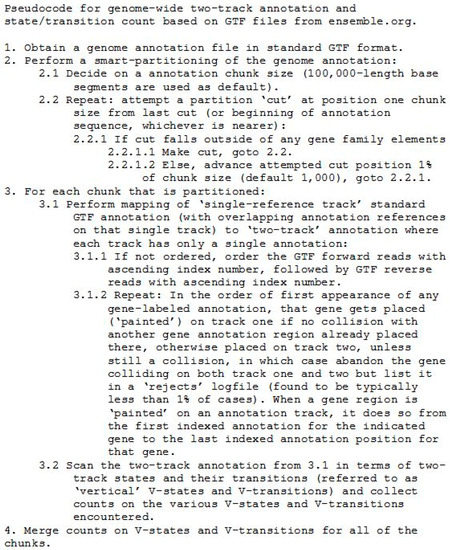
Figure 10.
Pseudocode for two-track annotation conversion from GTF, together with counting on two-track states and transitions.

Figure 11.
Track annotation conventions.
On each chunk of a given Chromosome being processed, two-track feature counts are then done in order to design the HMM, e.g., identify good states and transitions, or train the HMM, e.g., obtain prior probabilities on the various states and transitions, and profile HMMs for the bases emitted by those states and transitions. The pseudocode for counting on the different states and transitions found in the chunk under analysis is shown in Figure 10.
3.3. Two-Track Annotation and Counting—Order of Annotation Governs Track Placement
Figure 11 shows the two-track annotation conventions, where placement on track 1 is for the entirety of the first transcript from the GTF annotation file, and if another transcript has overlap with the first transcript it is placed on track 2. If further overlap occurs (requiring a third track) there are two conventions: (i) ignore third and higher overlapping transcript annotations, but record the location of the higher than 2nd order alt-splicing region; and (ii) mask the transcripts that have more than two overlaps and exclude from the counting analysis entirely. Since the occurrence of higher overlap order than two transcripts is rare (generally less than 5% in general, typically less than 1%), either convention works about the same insofar as the meta-state counts are concerned. In what follows, convention (i) is used.
Track placement info taken by itself cannot be used without trivial artifacts resulting from the ordering of the annotation information. Thus the need to pool counts with transitions from both track 1 and track 2. In other words, the V-transition counts on ‘ieii’ and ‘iiie’ (where ‘e’ is 0, 1, or 2), both describe ie overlap with ii and are pooled. Similarly for reverse reads, there is a further doubling of transitions when considering the reverse complement versions of the 3-prime-splice-site (ie → EI) overlap with alternative intronic (II).
4. Results
In Table 2 and Figure 12 are shown the results for the different types of alternative splicing described, along with the counts on start-of-coding, with extent of alternative splicing in the genome captured in terms of the ratio of alternative splicing events to the number start-of-coding events (the latter being the approximate number of genes). In Table 2, the V-transitions contributing to the counts on the different splice types are grouped as follows:
- (3′|i) V-transitions: i0ii, i1ii, i2ii, iii0, iii1, iii2, AIII, BIII, CIII, IIAI, IIBI, IICI.
- (5′|i) V-transitions: 0iii, 1iii, 2iii, ii0i, ii1i, ii2i, IAII, IBII, ICII, IIIA, IIIB, IIIC.
- (3′|e) V-transitions: 01i1, 12i2, 20i0, i020, i101, i202, AIAC, BIBA, CICB, BABI, CBCI, ACAI.
- (5′|e) V-transitions: 0i01, 1i12, 2i20, 010i, 121i, 202i, IABA, IBCB, ICAC, BAIA, CBIB, ACIC.

Table 2.
Counts on start-of-coding (j0 and Aj dimers) and on the different splice-sites. Altsum is the sum total of the different splice types (5′|i, 5′|e, 3′|i, and 3′|e). The last column ‘Alt/j0’ is the ratio of altsum to the {j0 + Aj} counts.

Figure 12.
The relative number of counts on start-of-coding (j0 and Aj dimers) and on the different splice-sites are shown in relation to each other. The charts, from left-to-right, are for the human, mouse, fly, and worm genomes.
Table 2 also summarizes the fraction of gene transcripts that have alternative splicing in the ‘Alt/j0’ column, where the # transcripts with alt-splicing is given in relation to the # transcripts total.
In Table 3 and Figure 13 are shown the counts for the different types of alternative splicing at the start of coding. Further discussion of the notation and results is in the Discussion section. In the table, {j0jj + jjj0}/j0 is the ratio of non-alt-splice starts to all starts. This partly captures the increased overall occurrence of alternative splicing since this would lead to more j0j0 counts and fewer j0jj. The start V-transitions marked with an ‘*’ have encumbered base-profiles in that the base statistics must be consistent with two types of consensus sequence, especially in the case of ‘j0i0’. Unencumbered starts would be: j0jj, j0j0 (overlapping starts, but both have same consensus), j0ii, j0II.

Table 3.
Counts on alternative splicing at the start-of-coding.

Figure 13.
The relative number of counts on alternative start-of-coding. The charts, from left-to-right, are for the human, mouse, fly, and worm genomes.
In Table 4 and Figure 14 are shown the counts for the different types of alternative splicing at the end of coding. Further discussion of the notation and results is in the Discussion section. In the table, {2jjj + jj2j}/2j is the ratio of non-alt-splice ends to all ends. This partly captures the increased overall occurrence of alternative splicing since this would lead to more 2j2j counts and fewer 2jjj. The start V-transitions marked with an ‘*’ have encumbered base-profiles in that the base statistics must be consistent with two types of consensus sequence, as before. Now see spliceosome mediated end variation as very common ({2jii + ii2j} = 2749 vs. 2j2j = 3442, so almost half of the alternative spliced genes in human have different ends).

Table 4.
Counts on alternative splicing at the end-of-coding.

Figure 14.
The relative number of counts on alternative end-of-coding. The charts, from left-to-right, are for the human, mouse, fly, and worm genomes.
5. Discussion
5.1. V–Transition Rules
In the counting on states shown in the Results, and discussed in what follows, we are working with the 25-transition (dimer state) model based off of the nine ‘primitive’ state model: j, i, I, 0, 1, 2, A, B, C. The 25 transitions that then follow are: jj, j0, jC, 2j, Aj; 01, 12, 20, BA, CB, AC, 0i, 1i, 2i, i0, i1, i2, AI, BI, CI, IA, IB, IC, ii, II. For vertical transitions (V-transitions) across tracks 1 and 2 there are thus 25 × 25 = 625 possible meta-states since there is no explicit constraint between tracks. Far fewer are seen in practice, however, due to the consistency constraints on overlapping splice-site signals, etc. Transitions overlapping with junk or intron are clearly allowed, so (25)jj, jj(25), ii(25), (25)ii, II(25), and (25)II, states are allowed (150 total) and the 4 × 12 = 48 transitions described in what follows for alt-splices overlapping with exon or intron, denoted (5′|e), (3′|e), (5′|i), and (3′|i) previously, are allowed, so expect to see at least 198 V-transitions. Of the 625 possible V-transitions many are never seen, however, and others are seen extremely rarely. This gives rise to 5 rules on allowed V-transitions involving splice sites, three rules on allowed V-transitions involving start-of-coding transitions, and two rules for the allowed V-transitions involving end-of-coding transitions:
- (1)
- Approximate frame agreement rule: j0 on track 1 cannot overlap 2j, 0i, 1i, i1, i2 on track 2, and only rarely overlap with 01 or 12 on track 2 (a consensus agreement rule). {j0, jC, 2j, Aj} similar, so excluding 4 × 5 = 20. Similarly with 01 track 1 not overlapping with 12, 20, 1i, 2i, i0, i2 on track 2 (rarely with j0 and 2j as noted). {10.12.20.BA, CB, AC} similar, so excluding 6 × 6 = 36 V–transitions. Similarly 0i on track 1 cannot overlap with j0, 2j, 12, 20, 1i, 2i, i0, i2 on track 2. {0i, 1i, 2i, i0, i1, i2, AI, BI, CI, IA, IB, IC} similar, so excluding 12 × 8 = 96 V-transitions.
- (2)
- No ‘eiie’ or ‘ieei’ rule (a consensus agreement rule): 0i on track 1 cannot overlap with i1. {0i, 1i, 2i, i0, i1, i2, AI, BI, CI, IA, IB, IC} similar, so excluding 12 × 1 = 12 V-transitions.
- (3)
- No exon boundary overlap with reverse coding region rule, where j0 cannot overlap BA, CB, AC, for example. {j0, jC, 2j, Aj} similar, so excluding 4 × 3 =12. Similarly 0i cannot overlap BA, CB, AC, and there are 12 splice types, so excluding 12 × 3 = 36. And, 01 cannot overlap jC, Aj, AI, BI, CI, IA, IB, IC, so 6 × 8 = 48 more exclusions. This appears to be a rule that shows that a coevolutionary linkage between cis or trans regulatory regions and reverse coding regions is highly unfavorable.
Of the 625 V-transitions possible, rules (1)–(3) reduce the types of V-transitions seen by 20 + 36 + 96 + 12 + 12 + 36 + 48 = 260, so down to 625 − 260 = 365 V-transitions thus far.
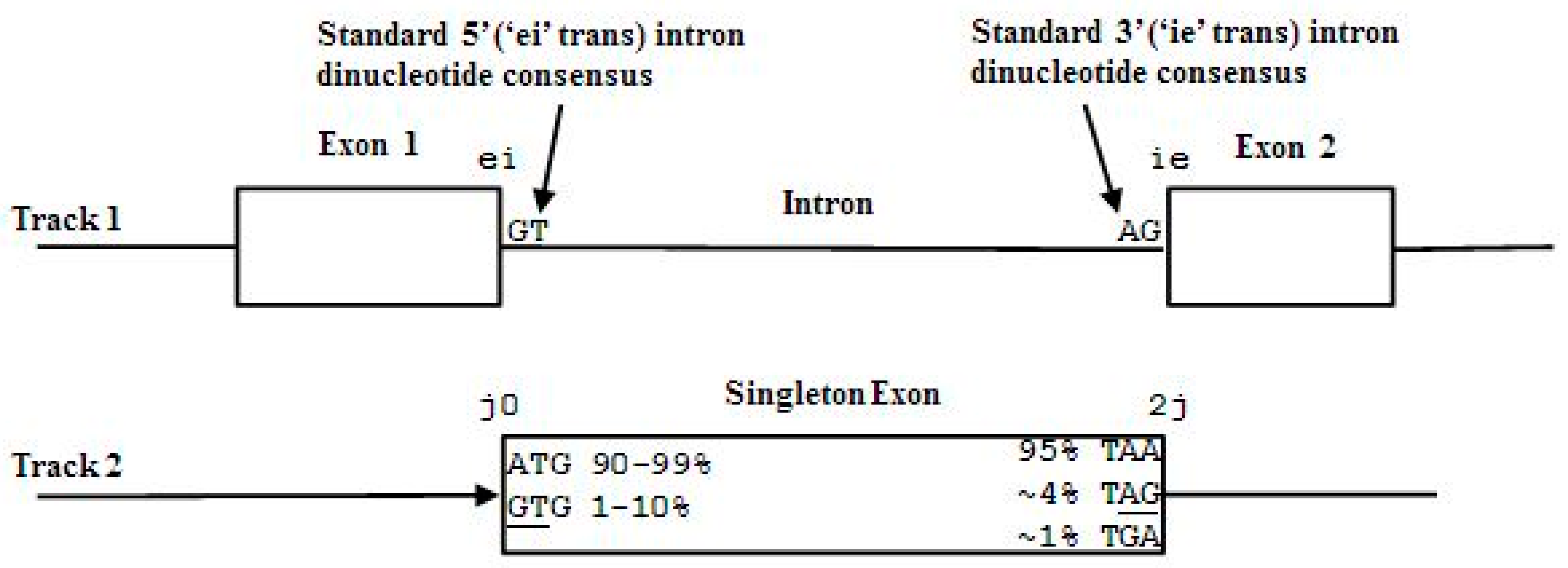
Since consensus agreement on overlapping signal types is a strong constraint, the question naturally arises as to when there is consensus agreement. Figure 15 shows examples of how eij0 and ie2j types of V-transitions can have consistent consensus sequences, thus giving rise to allowed V-transitions for these types of overlaps (and similarly for the reverse-read state transitions).
- (4)
- Start/End consensus disagreement rule: Figure 15 shows how consensus agreement is possible for ‘eij0’ and ‘ie2j’, but not for flipped consensus EIj0 or IEj0 or IE2j or EI2j (so twelve cases). When treating Aj and jC similarly to j0 and 2j, get another 12, for 24 V-transition exclusions total.
- (5)
- Avoid forward/reverse splice signal overlap. ‘0i’ cannot overlap AI, BI, CI; and would generally not favor overlap with IA, IB, IC. There are 12 × 6 = 72 similar exclusions.
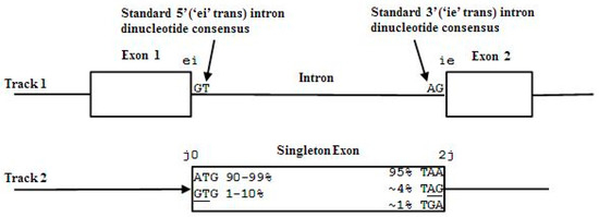
Figure 15.
The eij0 and ie2j types of V-transitions can have consensus agreement in their overlap, thus are allowed.
Starting from the 625 V-transitions possible, rules (1)–(5) reduce to 269 ‘likely’ V-transitions (although many are very rare, possibly with zero counts, as will be seen). Focusing on the start-of-coding and the end-of-coding allowed V-transitions as seen in the count data, further elaboration on the allowed V-transitions can be given. The start-of-coding (‘j0’) consensus rules, as seen in count data, appear to occur in three forms:
- (i)
- Zero counts found for: j0jC, j02j, j0Aj, jCj0, 2jj0, Ajj0 ➔ non-overlap with other start/end rule.
- (ii)
- Zero counts found for j0 overlap with reverse transitions except for II.
- (iii)
- Zero counts found for j0 overlaps with forward splice unless 3’ (dominated by base-frame 0 to be in agreement with 0 frame in ‘j0’).
As alternative splicing increases in usage across the genomes, expect both unencumbered alternative splicing (j0j0) and encumbered splicing (such as j0i0 and j020) to increase. Notably, the increase in j0i0 and j020 in more complex mammalian genomes, like mouse and human, indicates gene-growth that is probably spliceosome mediated by way of new first exon recruitment, as shown in Figure 16.

Figure 16.
Possible gene growth by way of new first exon recruitment.
The end-of-coding (‘2j’) consensus rules, as seen in count data, appear to occur in two forms:
- (I)
- Zero counts found for: j2j0, j20i, j21i, j2i0, j2i1, j2i2, indicating a non-overlap with other start/end or splice rule, except for 2j2i (end overlap with 5’splice appearing in more spliced genomes, and only in-frame, showing a slower growth in encumbered 2j versus encumbered j0, as with j0, have indications of spliceosomally driven alt-splice gene extension via exon recruitment from the trans-side of the gene).
- (II)
- Zero counts found for 2j overlap with reverse transitions except for II.
To a much smaller extent than seen at the start-of-coding cis region, spliceosome mediated growth also appears to occur directly via new terminus exon recruitment (shown as the alt-splice variant in the bottom-most annotation sequence shown in Figure 17).
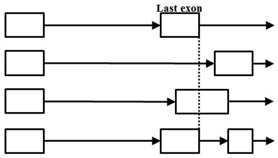
Figure 17.
End-of-coding alternative splicing, with the last case shown (bottom track) indicative of a process (possibly spliceosome mediated) for gene growth by way of new last exon recruitment.
5.2. Impact of Annotation Errors
In practice we see a small number of annotation errors, for example, in worm, the number of (normal) transition types seen is 31 (not the 25 theoretically possible), with the extra six (annotation error) transitions having very low counts: 1j = 7, ij = 14, 0j = 4, j1 = 4, ji = 28, j2 = 7 (where the smallest count on valid 25-group transitions is for Aj = 12,524 = jC). For worm, 251 non-zero count V-trans are seen, where the 31 base-state transitions are observed. Similarly, for fly 230 V-transitions are seen, with 33 base-state transitions; for mouse 324 V-transitions are seen, with 35 base-state transitions; and for human 351 V-transitions are seen, with 36 base-state transitions.
Of the 251 non-zero count V-transitions seen for worm, 61 are in the exclusion categories mentioned or involving non-25 transitions, all with extremely low counts, corresponding to annotation errors at a rate ~1/100,000. So only 190 ‘valid’ or non-exclusion V-transitions are seen for worm, some with very low counts, and some, evidently, zero due to ‘small’ sample size (e.g., 79 of the allowed, but very rare, 269 V-trans have 0 counts for worm). The larger genome sizes for mouse and human, on the other hand, appear to complete the sampling over likely transitions. If all 269 likely transitions are found in the human genome, this leaves 82 non-zero (but very low) counts in exclusion and annotation error categories.
6. Conclusions
A meta-state HMM implementation with 269 Vertical transitions, or two-track dimer states, is shown to suffice for performing a single-pass gene-structure identification that would capture (predict) almost all alternative splicing variants. Since roughly 70 of the possible V-transitions typically have either zero counts, or very low counts, modeling appears possible with only 200 two-track dimer states. The meta-HMM implementation described in [11] explored implementations with more states than this when working with larger footprint states, and did so using only a single workstation or laptop. Thus it is shown to be feasible to implement a meta-state HMM for alternative-splice gene structure identification without special computational requirements, and with sufficient statistical support (using roughly 200 two-track dimer states) for a strong model.
An analysis of the alternative splicing in a comparative genomics context reveals the expected increase in alternative splicing complexity as the organism becomes more complex, with the percentage of genes with alt-splice variants increasing from worm to fly to the mammalian genomes (mouse and human). Of particular note is an increase in alternative splicing variants at the start and end of coding with the mammalian genomes studied (mouse and human), allowing for new first exon and new last exon recruitment that is possibly spliceosome mediated. This suggests a possible mechanism for accelerated gene structure variation and selection in the mammals that is spliceosome mediated.
In future work we intend to implement the meta-HMM with the approximately 200 two-track dimer model using profile HMMs trained on base statistics for each of the dimer states. We will then use this tool in identifying genes shorter in length than allowed with the current cutoffs, as well as in identifying any regulatory motifs specific to particular types of alt-splice transitions, especially those that might be involved in exon recruitment.
Supplementary Materials
The following are available online at www.mdpi.com/2227-9709/4/1/3/s1.
Acknowledgments
The author would like to thank the Louisiana Board of Regents for research support. The author would also like to thank Meta Logos Inc., for research support and a research license. (Meta Logos Inc. was co-founded by the author in 2009; and Meta Logos Systems was founded by the author in 1997.)
Author Contributions
The code for the AGP feature extraction was written by SWH. Data runs and paper writing done by both S.W.-H. and A.J.L.
Conflicts of Interest
The authors declare no conflict of interest.
References
- Stanke, M.; Morgenstern, B. AUGUSTUS: A web server for gene prediction in eukaryotes that allows user-defined constraints. Nucleic Acids Res. 2005, 33, W465–W467. [Google Scholar] [CrossRef] [PubMed]
- Rajapakse, J.C.; Ho, L.S. Markov Encoding for Detecting Signals in Genomic Sequences. IEEE/ACM Trans. Comput. Biol. Bioinform. 2005, 2, 131–142. [Google Scholar] [CrossRef] [PubMed]
- Majoros, W.H.; Pertea, M.; Salzberg, S.L. TigrScan and GlimmerHMM: Two open source ab initio eukaryotic gene-finders. Bioinformatics 2004, 1, 2878–2879. [Google Scholar] [CrossRef] [PubMed]
- Taher, L.; Rinner, O.; Garg, S.; Sczyrba, A.; Brudno, M.; Batzoglou, S.; Morgenstern, B. AGenDA: Homology-based gene prediction. Bioinformatics 2003, 19, 1575–1577. [Google Scholar] [CrossRef] [PubMed]
- Altschul, S.F.; Gish, W.; Miller, W.; Myers, E.W.; Lipman, D.J. Basic local alignment search tool. J. Mol. Biol. 1990, 215, 403–410. [Google Scholar] [CrossRef]
- Sonnenburg, S.; Zien, A.; Ratsch, G. ARTS: Accurate recognition of transcription starts in human. Bioinformatics 2006, 22, e472–e480. [Google Scholar] [CrossRef] [PubMed]
- Do, J.H.; Choi, D.-K. Computational Approaches to Gene Prediction. J. Microbiol. 2006, 44, 137–144. [Google Scholar] [PubMed]
- Korf, I. Gene finding in novel genomes. BMC Bioinform. 2004, 5, 59. [Google Scholar] [CrossRef] [PubMed]
- Mathe, C.; Sagot, M.-F.; Schiex, T.; Rouze, P. Current methods of gene prediction, their strengths and weaknesses. Nucleic Acids Res. 2002, 30, 4103–4117. [Google Scholar] [CrossRef] [PubMed]
- Allen, J.E.; Majoros, W.H.; Pertea, M.; Salzberg, S.L. JIGSAW, GeneZilla, and GlimmerHMM: Puzzling out the features of human genes in the ENCODE regions. Genome Biol. 2006, 7 (Suppl. 1), S9. [Google Scholar] [CrossRef] [PubMed]
- Winters-Hilt, S.; Baribault, C. A Meta-state HMM with application to gene structure identification in eukaryotes. EURASIP J. Adv. Signal Process. 2010, 2010, 581373. [Google Scholar] [CrossRef]
- Winters-Hilt, S.; Jiang, Z. A hidden Markov model with binned duration algorithm. IEEE Trans. Signal Proc. 2010, 58, 948–952. [Google Scholar] [CrossRef]
- Winters-Hilt, S.; Jiang, Z.; Baribault, C. Hidden Markov model with duration side-information for novel HMMD derivation, with application to eukaryotic gene finding. EURASIP J. Adv. Signal Process. 2010, 2010, 761360. [Google Scholar] [CrossRef]
- Noguchi, H.; Park, J.; Takagi, T. MetaGene: Prokaryotic gene finding from environmental genome shotgun sequences. Nucleic Acids Res. 2006, 34, 5623–5630. [Google Scholar] [CrossRef] [PubMed]
- Kulp, D.; Haussler, D.; Reese, M.G.; Eeckman, F.H. A generalized hidden Markov model for recognition of human genes in DNA. Proc. Int. Conf. Intell. Syst. Mol. Biol. 1996, 4, 134–142. [Google Scholar] [PubMed]
- Van Baren, M.J.; Koebbe, B.C.; Brent, M.R. Using N-SCAN or TWINSCAN to predict gene structures in genomic DNA sequences. Curr. Protoc. Bioinform. 2007. [Google Scholar] [CrossRef]
- Rogic, S.; Mackworth, A.K.; Francis Ouellette, B.F. Evaluation of Gene-Finding Programs on Mammalian Sequences. Genome Res. 2001, 11, 817–832. [Google Scholar] [CrossRef] [PubMed]
- Dunham, I.; Shimizu, N.; Roe, B.A.; Chissoe, S. The DNA sequence of human chromosome 22. Nature 1999, 402, 489–495. [Google Scholar] [CrossRef] [PubMed]
- Burset, M.; Guigo, R. Evaluation of Gene Structure Prediction Programs. Genomics 1996, 34, 353–367. [Google Scholar] [CrossRef] [PubMed]
- Winters-Hilt, S.; Roux, B. Hybrid MM/SVM structural sensors for stochastic sequential data. In Proceedings of the Fifth Annual MCBIOS Conference. Systems Biology: Bridging the Omics, Oklahoma City, OK, USA, 23–24 February 2008. BMC Bioinform. 2008, 9 (Suppl. 9), S12. [Google Scholar]
- Liu, H.; Han, H.; Li, J.; Wong, L. DNAFSMiner: A Web-Based Software Toolbox to Recognize Two Types of Functional Sites in DNA Sequences. Available online: http://sdmc.i2r.a-star.edu.sg/DNAFSMiner/ (accessed on 26 June 2016).
- Sonnenburg, S.; Schweikert, G.; Philips, P.; Behr, J.; Rätsch, G. Accurate splice site prediction using support vector machines. BMC Bioinform. 2007, 8 (Suppl. 10), S7. [Google Scholar] [CrossRef] [PubMed]
- Degroeve, S.; Saeys, Y.; de Baets, B.; Rouzé, P.; van de Peer, Y. SpliceMachine: Predicting splice sites from high-dimensional local context representations. Bioinformatics 2005, 21, 1332–1338. [Google Scholar] [CrossRef] [PubMed]
- Muro, E.M.; Herrington, R.; Janmohamed, S.; Frelin, C.; Andrade-Navarro, M.A.; Iscove, N.N. Identification of gene 3’ ends by automated EST cluster analysis. PNAS 2008, 105, 20286–20290. [Google Scholar] [CrossRef] [PubMed]
- Bellora, N.; Farre, D.; Alba, M.M. PEAKS: Identification of regulatory motifs by their position in DNA sequences. Bioinformatics 2007, 23, 243–244. [Google Scholar] [PubMed]
- He, X.; Ling, X.; Sinha, S. Alignment and Prediction of cis-Regulatory Modules Based on a Probabilistic Model of Evolution. PLoS Comput. Biol. 2009, 5, 1–14. [Google Scholar] [CrossRef] [PubMed]
- Winters-Hilt, S.; Baribault, C. A novel, fast, HMM-with-Duration implementation—For application with a new, pattern recognition informed, nanopore detector. BMC Bioinform. 2007, 8 (Suppl. 7), S19. [Google Scholar] [CrossRef] [PubMed]
- Winters-Hilt, S. Hidden Markov Model Variants and their Application. BMC Bioinform. 2006, 7 (Suppl. 2), S14. [Google Scholar] [CrossRef] [PubMed]
- Lu, D. Motif Finding. Master Thesis, University of New Orleans, New Orleans, LA, USA, 2009. [Google Scholar]
- Shinozaki, D.; Akutsu, T.; Maruyama, O. Finding optimal degenerate patterns in DNA sequences. Bioinformatics 2003, 19 (Suppl. 2), ii206–ii214. [Google Scholar] [CrossRef] [PubMed]
- Frickey, T.; Weiller, G. Mclip: Motif detection based on cliques of gapped local profile-to-profile alignments. Bioinformatics 2007, 23, 502–503. [Google Scholar] [CrossRef] [PubMed]
- De Hoon, M.J.L.; Imoto, S.; Nolan, J.; Miyano, S. Open source clustering software. Bioinformatics 2004, 20, 1453–1454. [Google Scholar] [CrossRef] [PubMed]
- Wang, G.; Yu, T.; Zhang, W. WordSpy: Identifying transcription factor binding motifs by building a dictionary and learning a grammar. Nucleic Acids Res. 2005, 33, W412–W416. [Google Scholar] [CrossRef] [PubMed]
- Durbin, R.; Eddy, S.; Krogh, A.; Mitchison, G. Biological Sequence Analysis, Probabilistic Models of Proteins and Nucleic Acids; Cambridge University Press: Cambridge, UK, 1998. [Google Scholar]
- Rabiner, L.R.; Juang, B.H. An Introduction to Hidden Markov Models. IEEE ASSP Mag. 1986, 3, 4–16. [Google Scholar] [CrossRef]
- Winters-Hilt, S. Machine-Learning Based Sequence Analysis, Bioinformatics & Nanopore Transduction Detection; Lulu.com Publishing: Chapel Hill, NC, USA, 2011. [Google Scholar]
© 2017 by the authors; licensee MDPI, Basel, Switzerland. This article is an open access article distributed under the terms and conditions of the Creative Commons Attribution (CC BY) license ( http://creativecommons.org/licenses/by/4.0/).

