Abstract
Autonomous vehicles (AVs) are increasingly becoming a reality, enabled by advances in sensing technologies, intelligent control systems, and real-time data processing. For AVs to operate safely and effectively, they must maintain a reliable perception of their surroundings and internal state. However, sensor failures, whether due to noise, malfunction, or degradation, can compromise this perception and lead to incorrect localization or unsafe decisions by the autonomous control system. While modern AV systems often combine data from multiple sensors to mitigate such risks through sensor fusion techniques (e.g., Kalman filtering), the extent to which these systems remain resilient under faulty conditions remains an open question. This work presents a simulation-based fault injection framework to assess the impact of sensor failures on AVs’ behavior. The framework enables structured testing of autonomous driving software under controlled fault conditions, allowing researchers to observe how specific sensor failures affect system performance. To demonstrate its applicability, an experimental campaign was conducted using the CARLA simulator integrated with the Autoware autonomous driving stack. A multi-segment urban driving scenario was executed using a modified version of CARLA’s Scenario Runner to support Autoware-based evaluations. Faults were injected simulating LiDAR, GNSS, and IMU sensor failures in different route scenarios. The fault types considered in this study include silent sensor failures and severe noise. The results obtained by emulating sensor failures in our chosen system under test, Autoware, show that faults in LiDAR and IMU gyroscope have the most critical impact, often leading to erratic motion and collisions. In contrast, faults in GNSS and IMU accelerometers were well tolerated. This demonstrates the ability of the framework to investigate the fault-tolerance of AVs in the presence of critical sensor failures.
1. Introduction
Autonomous vehicles (AVs) are becoming more prevalent, with ongoing advancements bringing the industry closer to fully autonomous systems. As their integration into public roads accelerates, ensuring their safe operation becomes increasingly important. AVs have the potential to improve road safety [1], mobility, and environmental sustainability [2]. This transformation is driven by significant advances in sensing technologies, data processing, and intelligent control algorithms. In AV systems, sensor data serves as input for perception, localization, and decision-making processes. As such, the reliability of these sensors is critical for ensuring the safe and effective operation of autonomous vehicles.
Despite the increasing deployment of AVs in controlled environments and urban pilot programs, ensuring their safety in the face of real-world uncertainties remains a significant challenge. One particular challenge is the impact of sensor failures, which can arise due to environmental interference, hardware degradation, calibration errors, or cyber-physical attacks [3,4]. Sensor failures can lead to incorrect perception of the vehicle’s surroundings, degraded localization accuracy, or erratic control decisions, potentially resulting in catastrophic outcomes such as unsafe maneuvers or collisions.
Although the literature on autonomous vehicles extensively explores perception and control, relatively few studies have systematically simulated sensor failures in controlled environments to assess the fault tolerance of AV systems. Tools such as AVFI [5], CarFASE [6], and DriveFI [7] show promise in this regard, offering capabilities for structured fault injection, modeling sensor failures, and enabling reproducible experiments for behavior analysis. However, most published works [5,6,7,8,9,10] focus on algorithm development under ideal or mildly perturbed conditions, rather than on structured fault injection and behavior analysis of AV software stacks. This limitation is particularly significant when considered in the context of functional safety standards such as ISO 26262, which emphasize risk assessment and the validation of safety mechanisms under fault conditions [10]. Compliance with such standards requires not only theoretical resilience but also practical validation of a system’s response to component failures, namely sensors.
To address this gap, we propose a framework to assess sensor fault tolerance in AVs using simulation-based fault injection. The framework integrates CARLA, an open-source driving simulator capable of emulating sensor outputs in realistic urban environments, with Autoware, an open-source autonomous driving software stack. This integration allows for the execution of realistic urban driving scenarios under controlled conditions. A key component of this setup is the ROS bridge, which connects CARLA to Autoware by transmitting simulated sensor data. Sensor faults are injected through the ROS bridge by modifying sensor data in real time before it reaches Autoware. These include silent sensor failures (complete data loss) and noise (random deviations of sensor values) applied to LiDAR, IMU (gyroscope, accelerometer, and quaternion), and GNSS. Our contributions are summarized as follows:
- Integration of CARLA and Autoware: We established an integration that enables structured, automated testing of autonomous driving behavior under sensor failures using scenario-based simulations.
- Sensor Fault Injection Mechanism: We designed and implemented a fault injection system capable of simulating various sensor anomalies, including silent failures and noise. This mechanism targets key sensors such as LiDAR, IMU (gyroscope, accelerometer, and quaternion), and GNSS.
- Evaluation of AV System Response: We conducted a structured fault injection campaign to assess how Autoware responds under different sensor failure conditions. By injecting faults during scenario execution, we analyzed the system’s behavior and measured its ability to maintain safe and functional operation.
The remainder of this paper is structured as follows. Section 2 presents background concepts relevant to autonomous vehicles, including sensor systems, software architecture, and the foundations of sensor fusion. It also introduces the Autoware framework and the CARLA simulator. Section 3 reviews related work in AV fault injection and safety validation through simulation. Section 4 describes the simulation workflow and explains how sensor failures were implemented and executed within the test scenarios. Section 5 outlines the test conditions and fault model, followed by a description of each test run. Section 6 presents and analyzes the results. Finally, Section 7 concludes the study and discusses future work.
2. Background Concepts
To evaluate how autonomous driving systems respond to sensor faults, it is essential to understand the foundational components involved in their architecture and operation. This section introduces the key elements of autonomous vehicles, including their modular software architecture, sensor technologies, simulation environments, and the Autoware software stack. It begins by introducing different architectures of AV software, followed by a technical overview of the exteroceptive and proprioceptive sensors used in autonomous driving. The CARLA simulator and its integration with ROS are then presented as the tools used to emulate realistic driving scenarios. Finally, the Autoware system is described in terms of its architecture, sensing modules, and localization strategy. Together, these concepts provide the necessary context for understanding the simulation framework and fault injection methodology described later in this work.
2.1. Architecture of Autonomous Driving Systems
The Sense–Plan–Act (SPA) model has served as a conceptual foundation for autonomous systems, describing a sequential process of sensing, planning, and acting. While useful as a simplification, SPA is rarely used in its pure form for modern autonomous vehicles (AVs) because it struggles with real-time uncertainty, continuous adaptation, and highly dynamic road scenes. SPA’s reliance on static world models, absence of continuous feedback, and latency introduced by complete re-planning cycles make it less suited to real-time driving scenarios [11].
Modern AV software stacks adopt hybrid and reactive architectures, which blend fast feedback loops with higher-level deliberation. These designs often include multiple layers, reactive control, behavior sequencing, and planning, working in parallel and exchanging information continuously. Architectures such as Subsumption [12], Three-Tier (3T) [13], and Behavior Trees [14] are widely used in robotics, with adaptations for AVs. Additional advancements integrate Model Predictive Control (MPC) [15] for short-term re-planning, and learning-based perception–action loops for adaptive decision-making.
A common structure in AVs consists of Perception, Planning and Decision, Motion and Vehicle Control, and System Supervision modules [16]. These components operate in a tightly integrated loop, with frequent bidirectional data exchange and feedback paths, allowing for continuous adaptation to changing traffic conditions, sensor updates, and safety events. Figure 1 illustrates this modern modular organization.
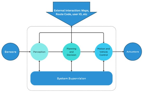
Figure 1.
Functional architecture of an autonomous driving system.
2.1.1. Perception
Prediction is responsible for interpreting sensor data to build an understanding of the vehicle’s surroundings. It receives data from sensors such as cameras, LiDARs, radars, ultrasonic sensors, IMUs, and GNSS, often combining these to improve resilience. Using this input, the perception software detects and classifies relevant environmental features: other vehicles, pedestrians, cyclists, road signs and traffic lights, lane markings, free space, obstacles, etc. It produces a structured world model or environmental representation, which may include the 3D positions and velocities of objects, their classifications (object types), traffic light states, and road geometry [17]. In short, perception “perceives” or senses the environment and answers the question: “What is around me and where?”.
Within perception, localization determines the position and orientation (pose) of the vehicle in the world. While perception builds a map of what is around the vehicle, localization answers the question “Where am I?”. The Localization module uses data from sensors such as GNSS for global position, inertial measurement units (IMU) for accelerations/rotational rates, and often uses features from perception (matching LiDAR scans or camera observations to a known map) to estimate the vehicle’s location with high accuracy. Localization operates continuously in the background, compensating for GNSS/IMU drift over time by incorporating environmental cues [18,19].
Perception also incorporates prediction, which predicts the future motion of dynamic objects in the environment. Given the current state of surrounding vehicles, pedestrians, or other moving agents (as perceived by the perception module), prediction algorithms estimate “What are they going to do next?”. This typically involves computing short-term trajectory predictions for each relevant object, for example, predicting that a vehicle in front will continue straight at a certain speed, or that a pedestrian might begin crossing the street [20].
2.1.2. Planning and Decision
The Planning and Decision modules determine the vehicle’s next actions based on the perceived environment, predicted object motion, and driving objectives. It processes data from perception and maps to decide on a safe and efficient course of action. In essence, the planning module answers the question “What should I do now?” by generating a trajectory or path that leads the vehicle toward its destination. This plan is computed with the end goal in mind and is continuously updated to adapt to the current situation, ensuring safety and compliance with traffic rules along the way [21]. In this context, the plan refers to the high-level driving decision (for example, taking a lane change or stopping at an intersection), while the trajectory specifies the detailed spatiotemporal path the vehicle should follow, including position, speed, and heading over time. The trajectory is generated to respect safety margins, comfort, and traffic rules, and it is continuously updated to adapt to changes in the environment.
2.1.3. Motion and Vehicle Control
The Motion and Vehicle Control module takes the planned trajectory or target command from the planning and decision module and executes it by sending low-level control inputs to the vehicle’s actuators (throttle, brake, and steering). Its role is to ensure the vehicle acts on the plan accurately and safely [22]. Control is commonly divided into lateral control (steering) and longitudinal control (acceleration and braking). Controllers rely on feedback from localization and onboard sensors to adjust commands in real time, closing the loop between planning and physical actuation [21,22,23].
2.1.4. System Supervision
Overseeing all the above modules is the System Supervision (also referred to as the vehicle management or coordination layer). This module monitors the overall operation of the autonomous driving system to ensure it functions safely and reliably [17,24]. The key responsibilities of system supervision are:
- Health Monitoring: The supervision module continuously checks the status of both hardware and software throughout the vehicle. If any module is not operating correctly, for example, a critical sensor drops out or the planner stops producing new trajectories, the supervision layer will detect this [17].
- Fault Management and Fail-Safe Mechanisms: Upon detecting an anomaly or failure, system supervision can initiate appropriate fail-safe mechanisms. This might mean alerting the driver or a remote operator or transitioning the vehicle into a safe state (such as gradually coming to a stop) if the autonomous system can no longer operate safely. This supervisory function is crucial for meeting functional safety requirements (ISO 26262 and similar standards) in a safety-critical system [17].
- Mission and Mode Management: It can manage transitions between autonomous driving and manual control, authorize engagement of self-driving when system checks pass, and abort or override the autonomy if necessary. It may also handle route initialization and high-level mission planning or interface with fleet management (in the context of robotaxis, for example), though these functions are sometimes considered separate. Additionally, system supervision can manage the Human–Machine Interface (HMI), for example, conveying system status to passengers or requesting driver takeover when needed [17].
This supervision module allows a complex AV software stack to maintain reliability, managing everything from fault diagnostics to system-level decision-making.
2.2. Sensors Used in AVs
Sensors used in autonomous vehicles can be classified into two categories: internal state sensors (proprioceptive sensors) and external state sensors (exteroceptive sensors) [25]. A survey of these sensor technologies, their roles, common failures, and mitigation strategies was presented in our previous work [26]. The remainder of this subsection summarizes the most relevant aspects for the fault injection study described in this article. Proprioceptive sensors are responsible for measuring the internal state of the vehicle. This group includes systems such as inertial measurement units (IMU), inertial navigation systems (INS), and encoders. Encoders provide critical feedback on components like steering, motor position, braking, and acceleration, enabling accurate assessment of the vehicle’s position, motion, and odometry [27].
Exteroceptive sensors gather information about the external environment. These include cameras, LiDAR sensors, RADAR, global navigation satellite systems (GNSS), and ultrasonic sensors, which enable the vehicle to perceive terrain, surrounding objects, and environmental conditions.
The following subsections describe the role and give an overview of each sensor type.
2.2.1. Ultrasonic Sensors
Ultrasonic sensors estimate distances and detect nearby objects by emitting high-frequency sound waves, typically between 20 and 40 kHz [28], which are beyond the range of human hearing. These sensors calculate distance based on the time-of-flight of the emitted sound wave, measuring the duration until the echo returns after reflecting off an object. Ultrasonic sensors are highly directional, with a narrow detection beam, which makes them suitable for short-range applications. They are most commonly used as parking sensors [29] and are effective in adverse weather conditions or dusty environments [3,30]. However, their operational range is limited, generally allowing obstacle detection only up to approximately two meters [30,31].
2.2.2. RADAR: Radio Detection and Ranging
Radar sensors operate by emitting electromagnetic signals and analyzing the reflected waves. In frequency-modulated continuous-wave (FMCW) radars, measuring the time delay between the transmitted and received signals yields the range to an object, while the Doppler shift provides its relative velocity [32]. They offer a wide perception range, typically from 5 m up to 200 m [31,33], and maintain reliable performance in adverse weather conditions such as rain, fog, or low-light environments. Radars are particularly effective at detecting nearby objects surrounding the vehicle with a high degree of accuracy [3,30,31,33].
However, radar systems can produce false positives due to signal reflections from surrounding structures. Additionally, FMCW automotive radars can experience mutual interference, particularly when many vehicles operate nearby, which has been documented experimentally and is an active area of mitigation research [34,35].
2.2.3. LiDAR: Light Detection and Ranging
LiDAR sensors estimate distance by emitting laser light and inferring range from the returned signal. LiDAR distance can be measured using time-of-flight, amplitude/phase-modulated continuous wave (AMCW/phase-shift), and frequency-modulated continuous wave (FMCW), ToF relies on round-trip time, AMCW estimates the phase shift in an intensity-modulated carrier, and FMCW uses coherent beat-frequency detection and can directly yield Doppler velocity [36,37,38,39,40]. By scanning multiple directions, they generate detailed spatial information in the form of point clouds and distance maps [41,42]. This high-resolution data allows for precise identification of objects, pedestrians, and environmental features, supporting functions such as obstacle avoidance and navigation. LiDARs operate in the near-infrared (e.g., around 905 nm or 1550 nm) and can detect objects at distances up to 300 m [41,42].
Under ideal weather conditions, LiDAR delivers superior spatial resolution compared to radar. However, its performance degrades significantly in adverse weather, such as fog, heavy rain, or snow, where light pulses are scattered or absorbed by particles in the air [30,31,42,43].
2.2.4. Camera
Cameras provide high-resolution visual data and can capture fine-grained details of the environment at distances of up to 250 m. They are widely used in autonomous vehicles for applications such as blind spot detection, lane change assistance, side view monitoring, and accident recording. When combined with deep learning algorithms, cameras enable the recognition and interpretation of traffic signs, road markings, vehicles, and pedestrians [44,45,46,47].
Despite their strengths, cameras are highly sensitive to changes in lighting and weather conditions, including rain, snow, and fog, which can significantly impair their performance. To compensate for these limitations, cameras are often used in conjunction with radar and LiDAR systems, enhancing overall perception accuracy and resilience [48].
2.2.5. GNSS
The operating principle of the GNSS relies on the receiver identifying signals from at least four satellites and calculating its distance to each one. Given that the satellite positions are known, the receiver uses trilateration to estimate its own position in global coordinates. While GNSS is a general term that encompasses multiple satellite constellations, such as the American GPS, the European Galileo, the Russian GLONASS, and the Chinese BeiDou, GPS (Global Positioning System) is often used to refer to all satellite-based positioning systems.
GNSS signals are prone to many errors that reduce the accuracy of the system, including the following:
- Clock bias and synchronization, due to residual satellite-clock error and receiver clock drift/jitter, clock/synchronization effects are present, but the receiver’s absolute bias is estimated with (x, y, z), so stability, not absolute offset, governs positioning accuracy [49].
- Signal delays, caused by propagation through the ionosphere and troposphere.
- Multipath effect.
- Satellite orbit uncertainties.
Current vehicle positioning systems improve their accuracy by combining GNSS signals with data from other vehicle sensors (e.g., inertial measurement units (IMU), LiDARs, radars, and cameras) to produce trustworthy position information [50,51,52]. This mitigation strategy is called sensor fusion and is discussed in Section 2.2.7. GNSS is susceptible to jamming, such as when the receiver encounters interference from other radio transmission sources. GNSS receivers also suffer from spoofing, when fake GNSS signals are intentionally transmitted to feed false position information and divert the target from its intended trajectory.
2.2.6. Inertial Measurement Units
Inertial Measurement Units consist of multiple sensors, typically accelerometers, gyroscopes, and magnetometers. These sensors provide measurements of linear acceleration, angular velocity, and magnetic orientation. Based on this data, the system estimates the movement and orientation of the vehicle in three-dimensional space. The orientation is often expressed using quaternions, which offer a stable and precise representation of rotation. IMUs play a key role in detecting slippage, lateral movement, and changes in direction. When combined with other sensors such as GNSS or LiDAR, the IMU contributes to inertial guidance, a method that helps correct positioning errors and enhances the accuracy and frequency of vehicle motion estimation [31,52].
2.2.7. Sensor Fusion
Sensors vary in technology and purpose, and each type of sensor has its weaknesses that are inherent to its technological capabilities. To cover these weaknesses, some mitigation strategies are implemented, such as sensor fusion [24]. Sensor fusion is a crucial part of autonomous driving systems [27,32] where input from multiple sensors is combined to reduce errors and overcome the limitations of individual sensors. As cameras offer high-resolution images suitable for object classification and lane detection, LiDAR excels at precise distance measurements and accurate spatial mapping, radar provides reliable distance and velocity measurements under adverse conditions, and GNSS offers global positional data, combining information from these diverse sources allows autonomous vehicles to enhance overall perception performance and resilience, especially when individual sensors are compromised due to faults, noise, or environmental conditions [17,24,52].
Sensor fusion is crucial for ensuring AV safety, as reliance on a single sensor often leads to vulnerabilities and reduced performance under real-world conditions. Through the fusion process, redundancy across sensor modalities can be leveraged to compensate for inaccuracies or intermittent sensor failures, thereby increasing overall system resilience.
In autonomous driving stacks, such as Autoware, sensor fusion often occurs at multiple abstraction levels, depending on specific module requirements. Autoware applies Kalman filtering techniques to fuse GNSS positional data with LiDAR-based localization estimates, enhancing accuracy and reducing localization uncertainty, even under sensor noise or faults. Kalman filters are probabilistic algorithms particularly suited for sensor fusion because they efficiently handle noisy data, dynamically update estimates based on incoming measurements, and predict future system states.
The extensive literature on sensor fusion emphasizes its interdisciplinary complexity, involving classical algorithms (e.g., Kalman filtering, particle filtering, Bayesian inference) and modern deep-learning approaches [17,24,32,46,50,51,52,53,54,55,56,57,58,59,60,61,62,63,64,65,66,67,68,69,70,71,72,73,74]. However, a detailed review of these methods falls beyond the scope of this study, as our primary goal is to assess system behavior under sensor faults rather than optimizing or developing fusion techniques.
2.3. CARLA
Autonomous driving technology relies on simulation environments to validate and enhance safety and performance before real-world deployment. These environments replicate real-life urban scenarios, integrating entities like vehicles, pedestrians, and complex infrastructure elements. The focus of these simulations is the ego vehicle, which represents the autonomous vehicle under study, interacting dynamically within the simulated environment. The ego vehicle’s behavior is managed through decision-making algorithms, forming a closed-loop system where sensor data of the ego vehicle is sent to the autonomous driving algorithm, and subsequently, the algorithm controls the ego vehicle. After evaluating several existing simulators and open-source autonomous driving stacks, CARLA was selected due to its realistic urban environments, sensor simulation capabilities, and ease of integration.
CARLA (Car Learning to Act) is an open-source simulator designed for autonomous driving research and development. Developed by the Computer Vision Center (CVC) at the Universitat Autònoma de Barcelona, CARLA provides a realistic 3D environment for testing and validating autonomous driving systems under a wide range of conditions. It supports high-fidelity urban scenes, configurable weather, traffic actors, and a broad suite of sensors, making it a widely adopted tool in both academic and industrial settings. The simulation platform supports flexible setup of sensor suites and provides signals that can be used to train driving strategies, such as GNSS coordinates, speed, acceleration, and detailed data on collisions and other infractions. A wide range of environmental conditions can be specified, including weather and time of day.
CARLA is built on Unreal Engine 4, which allows for advanced rendering and physics simulation (a new version is being built using Unreal Engine 5). The simulator operates using a client–server architecture (Figure 2) where:
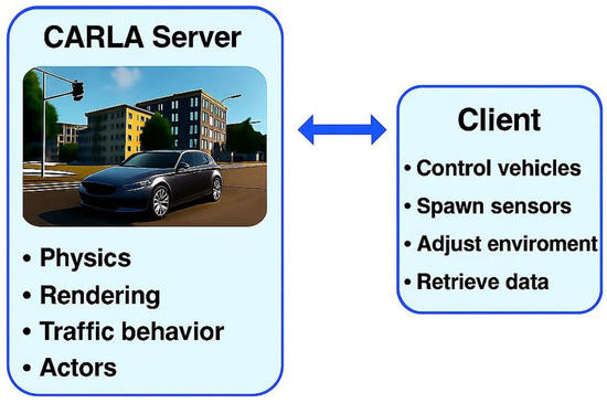
Figure 2.
CARLA-Client communication using its API.
- The CARLA server handles the simulation environment, including physics, rendering, traffic behavior, and all the actors in the scene.
- The client, which may use a TCP/IP API or operate through a ROS interface, communicates with the server to control vehicles, place sensors, modify environment settings, and access simulation data.
CARLA can operate in two simulation modes: asynchronous and synchronous [75]. In the default asynchronous mode, the server advances the simulation independently of the client, meaning that events and sensor data generation depend directly on the computing speed of the machines involved. This can introduce non-deterministic behavior, as faster or slower hardware affects the timing of events, potentially leading to inconsistencies across simulation runs.
The synchronous mode ensures determinism and repeatability. In this mode, the simulation advances strictly in lockstep with the client’s commands, and each simulation step only progresses when explicitly triggered by the client. Thus, simulation events occur based on virtual time, independent of how long the hardware takes to compute each step. Consequently, a slower machine will take more real-world time to complete the same number of simulation steps compared to a faster machine. However, the internal timing, precision, and order of events within the simulation remain consistent. The concept of virtual time is crucial in this context, as it ensures simulation integrity and repeatability, making synchronous mode particularly suitable for experiments where deterministic and precise timing control is required.
2.3.1. Scenario Management and Ego-Vehicle
Scenario creation is facilitated by tools such as the Scenario Runner, which allows for the definition and control of events including intersections, pedestrian crossings, emergency stops, and vehicle overtaking. These scenarios define not only the behaviors and trajectories of multiple actors in the simulation, but also the environmental conditions (such as weather or time of day).
At the core of each scenario is the ego vehicle, representing the autonomous vehicle under test. It can be configured with a wide range of sensors including LiDAR (standard and semantic), RGB and depth cameras, IMU, GNSS, radar, and dynamic vision sensors (DVS). These sensors are placed at configurable locations on the vehicle and stream data in real-time, enabling both online and offline analysis. The ego vehicle can be controlled manually via the client interface or connected to an external autonomous driving system such as Autoware.
Scenario Runner is a Python-based framework developed specifically for CARLA that enables the execution of these driving scenarios. It provides an interface for defining scenario behavior, controlling the timing and logic of actor actions, and monitoring simulation outcomes. Scenario descriptions can be written in Python scripts or in XML format, allowing for a modular and reusable setup.
Once a scenario is launched, Scenario Runner connects to the running CARLA server using the Python API (Python 3.7). It then spawns the defined actors into the simulation world, orchestrates their behavior over time, and monitors key criteria such as collisions, route completion, traffic light compliance, and other successful conditions. This enables repeatable and automated testing of AV behavior under consistent environmental and situational parameters, which is essential for evaluating performance and safety under diverse and controlled conditions.
2.3.2. CARLA—Autonomous Driving System Communication Using ROS
The CARLA ROS Bridge functions as a middleware interface that facilitates the integration of the CARLA simulation environment with ROS, enabling communication between the ego vehicle simulated in CARLA and external autonomous driving software frameworks.
ROS is an open-source middleware framework widely adopted in robotics research and development. It offers a modular architecture based on a publish–subscribe communication model, wherein distributed software components, referred to as nodes, exchange information through topics. ROS additionally provides comprehensive tools for sensor integration, data visualization, debugging, and simulation control. Figure 3 is a simplified diagram of the communication between CARLA and Autoware.
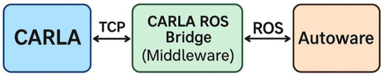
Figure 3.
CARLA ROS bridge Diagram.
Within the domain of autonomous driving, ROS links core modules such as perception, localization, planning, and control subsystems. The CARLA ROS bridge translates CARLA’s internal simulation data into standard ROS message formats and vice versa. This bidirectional interface enables the deployment of advanced driving stacks, such as Autoware, within the simulated environment. CARLA ROS bridge core functionalities include:
- Providing Sensor Data (Lidar, Semantic lidar, Cameras, GNSS, Radar, IMU)
- Providing Object Data (Traffic light status, Visualization markers, Collision, Lane invasion)
- Controlling AD Agents (Steer/Throttle/Brake)
- Controlling CARLA (Play/pause simulation, Set simulation parameters)
This integration is essential for testing and validating autonomous driving algorithms, particularly under controlled fault conditions.
2.4. Autoware
Autoware is an open-source software stack for autonomous driving systems, built on top of ROS, supporting both ROS 1 (Autoware.AI) and ROS 2 (Autoware.Auto/Autoware.Universe), with the newer ROS 2-based versions focusing on real-time safety, modularity, and compliance with automotive-grade standards. We have selected Autoware as our autonomous driving system to test our framework for its modular open-source architecture, active community support, and compatibility with ROS-based simulation frameworks.
Autoware builds on ROS by integrating a curated set of perception, localization, planning and control modules tailored for autonomous driving. Compared with using ROS alone, Autoware provides a standardized interface to vehicle hardware, built-in sensor fusion pipelines (e.g., LiDAR/IMU/GNSS fusion), high-definition map support, object detection and tracking, behavior and trajectory planning, and vehicle control interfaces.
Autoware is designed to serve as a complete platform for research, prototyping, and deployment of self-driving vehicles, particularly in urban and suburban environments [76], and when integrated with CARLA, Autoware becomes a powerful tool for testing, validation, and development in a safe and reproducible virtual environment.
Autoware has been successfully deployed in various real-world autonomous driving projects, especially in Japan and Europe, including autonomous shuttles, delivery robots, and smart city infrastructure tests [77].
2.4.1. Architecture
Autoware provides a modular architecture (Figure 4) that includes all the essential modules required for autonomous vehicle operation, such as:
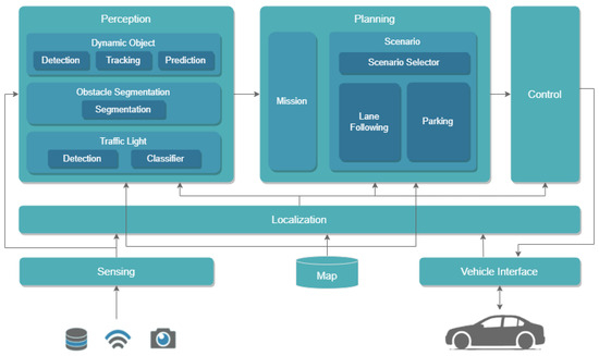
Figure 4.
Autoware Architecture [76].
- Perception: Object detection, segmentation, and tracking using data from LiDAR and cameras.
- Localization: Using GNSS, IMU, and LiDAR-based SLAM (Simultaneous Localization and Mapping) or map-matching for accurate vehicle positioning.
- Planning: Path planning, behavior planning, and route generation based on real-time map and object data.
- Control: Low-level vehicle actuation commands, such as throttle, brake, and steering, which are received by the vehicle interface responsible for executing them through actuators.
- Interface: Tools for vehicle-to-platform communication and human–machine interaction.
2.4.2. Sensing
The sensing module (Figure 5) applies pre-processing to the raw sensor data required by each module. It also abstracts data formats to allow the usage of sensors from different brands.
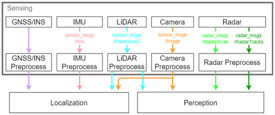
Figure 5.
Autoware sensing module.
This pre-processing includes applying filters, calibrating sensor inputs, and converting them into standardized message formats. The goal is to abstract away vendor-specific differences and provide clean, structured data for downstream modules like localization, perception, and control.
- GNSS: Provides global positioning (latitude, longitude, altitude) and orientation information. It is used primarily for global localization and navigation.
- IMU: Supplies measurements of vehicle motion, including acceleration and angular velocity. This data supports orientation tracking and is essential for sensor fusion techniques.
- LiDAR: Generates detailed 3D representations of the vehicle’s surroundings. It is used for localization (e.g., scan matching) and object detection.
- Camera: Delivers visual information for scene understanding, such as lane markings, traffic lights, and object classification.
- Radar: Detects objects by measuring distance, speed, and direction. Its robustness to adverse weather makes it valuable for tracking other road users.
Each of these sensors contributes complementary information that, once processed, supports the vehicle’s perception and decision-making systems.
2.4.3. Map
Autoware uses high-definition maps to support localization, routing, traffic rule handling, and to provide context for prediction and control. Two complementary map types are used: a vector map that encodes road semantics and a point cloud map that provides dense three-dimensional geometry.
The vector map is represented in Lanelet2 format. It contains lane geometry and topology, speed limits, turn permissions, stop lines, crosswalks, and traffic lights and signs. Behavior planning builds a lane graph from this information and triggers situation-specific modules such as lane change and intersection handling. Velocity planning reads speed limits and curvature from the map to set safe speed profiles and approach speeds.
The point cloud map provides a georeferenced three-dimensional model of the static environment, including road surface, curbs, building facades, poles, and barriers. It is used primarily for LiDAR-based localization through scan matching, for example, with NDT. Perception can also use the point cloud to remove the ground, mask static structures, and improve obstacle segmentation.
Both maps live in the fixed map frame in a local ENU coordinate system. A small projection metadata file specifies the transform from WGS84 latitude and longitude to this local frame so that GNSS positions are consistent with LiDAR and map coordinates.
Vector maps are authored and validated with Lanelet2 tools, while point cloud maps are built from survey LiDAR or SLAM runs and downsampled for runtime use. At startup, map loader nodes publish both maps, and large point clouds can be tiled and streamed so that only the needed tiles are kept in memory.
At runtime, localization aligns live LiDAR scans to the point cloud map and may fuse the resulting pose with GNSS and IMU. Routing and behavior planning query Lanelet2 topology and regulatory elements to generate routes and make right-of-way decisions. Velocity planning enforces map-based limits and approach constraints. Perception and prediction use both geometry and semantics to aid segmentation and provide intent context. Accurate alignment between the vector map, the point cloud map, and the real scene is critical. Otherwise, if misaligned, it can degrade localization quality and lead to poor decisions downstream. In summary, the map outputs the following:
- To the sensing module, the projection information (used to convert GNSS data to the local coordinate system).
- To the localization module, the point cloud (used for LiDAR-based localization) and vector maps (used for localization methods based on road markings).
- To the perception module, the point cloud map (used for obstacle segmentation) and vector map (used for vehicle trajectory prediction).
- To the planning module, the vector map (for behavior planning).
2.4.4. Localization
The localization module estimates the vehicle pose in the map frame and provides velocity and covariance in real-time. It ensures that these estimations are reliable, and if not, it generates errors or warning messages to inform the error-monitoring system. The method used for localization depends on the available sensors and the characteristics of the environment.
One commonly used method involves combining 3D LiDAR with a point cloud map. This approach is particularly effective in urban settings where numerous buildings and structures provide distinctive features for alignment. It works by matching incoming LiDAR data with a pre-existing point cloud map using techniques such as scan matching or Normal Distributions Transform. However, this method performs poorly in environments where the map lacks structural features, such as rural landscapes, open highways, or tunnels. It is also sensitive to environmental changes not represented on the map, including snow, construction work, or structural alterations. Signal issues such as reflections, glass surfaces, or interference from other laser sources may further degrade accuracy.
Another supported method involves using either 3D LiDAR or a camera in combination with a vector map. This configuration performs well in environments with clearly marked lanes, such as highways. Its accuracy can be affected by degraded or obstructed lane markings and variations in road surface reflections.
GNSS-based localization is suitable for open environments with minimal obstructions, such as rural areas. While it provides absolute global positioning, it is vulnerable to signal degradation, blockage, and spoofing. IMU-based localization relies on measurements of acceleration and angular velocity to estimate pose changes through dead reckoning. It works well in smooth and flat road conditions, but it is subject to drift over time due to inherent sensor biases which can be affected by environmental conditions such as temperature.
The Localization module integrates data from all these sources to improve accuracy and resilience. It requires that all incoming sensor data be correctly timestamped, valid, and consistent with the vehicle’s configuration. Additionally, maps used for localization, such as point cloud or lanelet2 formats, must closely match the real environment and be aligned if multiple sources are used. Large discrepancies between the map and the actual scene may lead to localization errors.
2.4.5. Perception
In Autoware, data from LiDAR, cameras, and radar are time-aligned with the vehicle’s pose and the map. The pipeline starts with point-cloud pre-processing (pointcloud_preprocessor), which removes noise, downsamples the cloud, crops to the area near the car, and separates ground from obstacles. Basic checks make sure timestamps and sensor calibrations are consistent, and map information (Lanelet2 plus the point-cloud map) gives extra context.
For LiDAR-based object detection, Autoware provides two options. The learning-based path, lidar_centerpoint, runs a modern 3D neural network (CenterPoint with a PointPillars backbone) and outputs oriented boxes for cars, pedestrians, and other objects. It is accurate and works well in busy scenes. The classical path, autoware_euclidean_cluster, does not use a neural network. Instead, it groups nearby points into clusters after simple filtering. It is fast, light on compute, and useful on modest hardware.
Perception then tracks objects over time, so they do not “blink” in and out when sensors are noisy. The multi_object_tracker combines consecutive detections (and multiple sensors when available) to keep a stable ID, position, and velocity for each object. When camera detections are enabled, autoware_bytetrack can track image-space boxes, and autoware_detection_by_tracker can feed the tracker’s estimates back to the detector to smooth things further.
Traffic light handling uses the map to narrow the camera’s search to only the signal heads that matter for the current lane. A detector (traffic_light_fine_detector) reads the light bulbs and their states, and a small association step ties them to the correct Lanelet2 signal group and stop line so planners can react at the right place.
Finally, Autoware produces a drivable-space/costmap that marks where the vehicle can safely drive. It uses the filtered LiDAR geometry, masks out known static structures with the point-cloud map, and inflates obstacles by a small safety margin. Parameters (for example, voxel size, cluster tolerances, detector confidence thresholds, and update rates) let users trade accuracy, smoothness, and runtime to match their compute budget and operating domain.
To cope with bad conditions, perception includes health checks. If a sensor drops frames or becomes unreliable, LiDAR glare or camera saturation, the system can down-weight that source, fall back from the learned detector to clustering, tighten tracking gates, or signal “degraded perception” so the vehicle can slow down or stop.
2.4.6. Planning
The Planning module determines where and how the vehicle should move based on the current environment, mission objectives, and safety constraints. It is structured into three main submodules: mission planning, planning modules, and validation. This modular architecture allows developers to extend or replace individual modules according to specific requirements or advancements.
First, mission (route) planning computes a global route from the current position to the destination using the Lanelet2 road graph. The output is a sequence of lanelets and waypoints that downstream modules follow. If the destination changes or a road becomes unavailable, the route is recomputed. Next, behavior planning decides what maneuver to perform along that route. Depending on rules and context, it may keep lane, change lanes, stop at a stop line, yield at an intersection, slow for a crosswalk, or pull over. It uses lane topology, speed limits, right-of-way, and traffic-signal states from the map and perception. In Autoware, these behaviors are provided as modular plugins so projects can enable only what they need. Then, motion planning turns the chosen behavior into a smooth, time-stamped trajectory. It produces a path (position and heading over distance) and a velocity profile (speed, acceleration, and jerk) that respect vehicle limits and passenger comfort. For low-speed areas and tight spaces, a freespace planner (e.g., Hybrid-A*) can generate drivable paths without relying on lane centerlines. An avoidance component can also shift the path laterally to pass slow or stopped obstacles when rules allow.
A velocity planning and smoothing stage enforces speed limits, approach speeds at intersections and crosswalks, lateral acceleration bounds from curvature, and safe gaps to lead vehicles. Smoothing shapes acceleration and jerk so the trajectory is comfortable and trackable by the controllers.
Before handing the trajectory to control, safety and feasibility checks verify that it stays within drivable space, avoids collisions with the latest obstacles, and respects speed and curvature limits as well as the selected behavior (for example, stopping before the stop line). If a check fails, the planner slows down, stops, or re-plans.
Planning consumes detected objects and traffic-signal states from perception, the current pose and velocity from localization, and the global route from mission planning. It outputs a time-stamped trajectory for control to track and publishes status so supervision can react if planning degrades (for example, by requesting a slow-down or stop).
2.4.7. Control
The Control module in Autoware is responsible for translating planned trajectories into low-level commands that can be executed by the vehicle’s actuators (steering, throttle, and brake), meaning that the goal of the control module is to track the target trajectory with stable lateral steering and longitudinal speed control. Autoware provides two main lateral controllers. The Pure Pursuit controller is a geometric look-ahead tracker that is robust and simple to tune, making it a common choice at low and medium speeds. The MPC Lateral controller picks the steering command by solving a small optimization problem at each time step. It uses a simple (linearized) vehicle model and a quadratic program solver, and lets you set explicit limits on steering rate and path curvature. The module also includes practical tuning guidance (e.g., horizon length and weight settings) so you can balance tracking accuracy and smoothness. Autoware’s PID Longitudinal controller combines feedforward and feedback acceleration, with options for slope compensation and delay handling. It tracks the velocity profile produced by the upstream planners and aims to deliver smooth speed regulation under typical driving conditions.
2.4.8. Vehicle Interface
The Vehicle Interface serves as the intermediary between the control commands generated by Autoware and the vehicle’s physical actuators or, in this case, the simulated vehicle provided by CARLA. It translates high-level commands, such as steering angle, throttle percentage, brake pressure, and gear selection, into actuator-level signals that the simulation environment can interpret and execute. CARLA is responsible for simulating the dynamics and responses of the ego vehicle based on the received control inputs.
2.5. Fault Injection in AV Systems
Fault injection is a testing technique where faults or errors are deliberately introduced into a system to evaluate its behavior and fault-tolerance capabilities [78]. In the context of autonomous vehicles, fault injection can target hardware (e.g., CPU errors), software (bugs), sensor data, or communications. Our focus is on sensor fault injection, which falls under software-implemented fault injection by corrupting sensor outputs, simulating the failure of the sensors. The motivation for fault injection in autonomous vehicles lies in the need to evaluate system safety under failure conditions. While standards such as ISO 26262 emphasize the importance of analyzing and validating the system’s behavior across different fault modes, implementing these tests in real-world settings is costly, risky, and often unfeasible. Although inducing faults directly in hardware components, such as damaging sensors or interfering with signals, can be a valid fault injection approach, doing so on real vehicles poses serious safety hazards and financial implications. Simulated fault injection offers a safe, controlled, and repeatable alternative that enables researchers and engineers to evaluate fault tolerance mechanisms without endangering people or damaging equipment. By using a simulator, we can expose the autonomous driving system to rare or dangerous scenarios that would be too risky in the real world. This includes extreme sensor failures like a completely blinded camera or a wildly drifting IMU, which could be life-threatening on a real vehicle but can be studied harmlessly in simulation.
3. Related Work
The safety validation of autonomous vehicles (AVs) has become a crucial research topic due to the increasing complexity of AV systems and the critical role sensors play in ensuring their reliable operation. The existing literature has focused on developing frameworks and simulation tools to systematically assess AV resilience under sensor faults, as well as evaluating AV performance in controlled virtual environments.
This section reviews prior work organized into two main categories: fault injection frameworks for AV safety validation and simulation-based AV testing. We highlight the strengths and limitations of these studies, clarifying the unique contributions of our research.
3.1. Fault Injection in Autonomous Vehicles
Ensuring that autonomous vehicles can handle faults has led to a body of research on AV fault injection and dependability assessment. One of the early efforts is AVFI (Autonomous Vehicle Fault Injector) [5], which pioneered end-to-end fault injection in AV systems. AVFI introduced faults at various points: sensor inputs (e.g., simulating camera or LiDAR failures), internal processing (e.g., flipping bits in a neural network), and even actuator commands, all within a simulated driving environment. The tool measured domain-specific safety metrics such as mission success rate and number of traffic violations under each fault scenario. Preliminary results from AVFI showed that injecting faults could indeed cause an AV to commit traffic violations that would not otherwise occur, underlining the importance of testing AVs beyond nominal conditions. AVFI used the CARLA simulator as a basis, demonstrating CARLA’s suitability for such fault experimentation [5].
Building on this, researchers have looked for smarter ways to inject faults. DriveFI (proposed by researchers at NVIDIA in 2019) [7] is a machine learning-based fault injection engine. Instead of manually specifying faults, DriveFI employs a Bayesian optimization approach to automatically discover the most “dangerous” faults and scenarios. By testing two industry-grade AV stacks (including NVIDIA’s own and Baidu’s Apollo), DriveFI was able to find hundreds of safety-critical vulnerabilities within hours, whereas random fault injection over weeks found few or none. The types of faults considered included sensor distortions and even logic bugs, and the impact was measured in terms of accidents or near-collisions in simulation. This work highlights how broad the space of possible faults is, and the need for intelligent search methods to focus on impactful cases [7].
The CarFASE tool [6] is specifically designed to integrate with open-source driving stacks (like OpenPilot by Comma.ai) and evaluate their behavior under both accidental faults and malicious attacks. For example, CarFASE can simulate a sudden change in camera brightness to mimic sensor attacks and then observe how the driving policy reacts. The authors used CarFASE to test OpenPilot’s resilience, and one use case showed that increased brightness (simulating a camera blinding scenario) led to degraded lane-keeping performance. The platform provides a library of fault models and a campaign configurator to automate scenario runs. The emergence of CarFASE underscores the community’s interest in accessible tools for fault injection using popular simulators like CARLA.
Aside from these, other works have explored particular sensor fault scenarios. Another work [48] focused on camera failures in an AV context, defining failure modes such as blurred images, blackout, and occlusions, and testing their effect on object detection and a self-driving agent in a simulator. The results showed that certain camera failures significantly increase detection errors and can lead to collisions in the simulation, which reinforces the notion that redundancy (like having multiple cameras or additional sensors) is needed. There are also studies on injecting faults in ADS controllers or code (for instance, using fuzzing or software mutation), but those are beyond the scope of sensor-level fault injection that we emphasize.
In contrast to prior AV fault injection studies that often focus on isolated algorithms, single sensors, or open-loop data perturbations, this work delivers a closed-loop, scenario-triggered fault injection framework operating at the middleware level of a full autonomous driving software stack. The framework supports multiple sensor types (LiDAR, IMU gyroscope/accelerometer/quaternion, GNSS), and uses a structured and reproducible fault model with location, type, trigger, and duration dimensions. By running injections during complete simulated driving scenarios, we capture system-level behavior and safety outcomes, enabling consistent classification of whether a fault was tolerated or led to unsafe operation. This combination of closed-loop execution, multi-sensor scope, and reproducibility distinguishes our work from previous tools and studies. Furthermore, our framework is implemented on ROS 2, which is mostly used in university research, but it can be ported to AUTOSAR Adaptive by bridging ROS 2 topics to SOME/IP (ara::com) services. Recent work [79] proposes an integrated ROS 2–AUTOSAR architecture (ASIRA) with a ROS 2–SOME/IP bridge and demonstrates data exchange in autonomous driving scenarios, including Autoware interoperating with an Adaptive AUTOSAR simulator, providing a path to use our framework on production-oriented AV software stacks. In practice, porting requires mapping message schemas and QoS/timing semantics and implementing an AUTOSAR-native injector; we list this engineering as future work. While our experiments run on a ROS 2 stack, the approach can be directly relevant to AUTOSAR-based developments and transferable to production-oriented pipelines.
In summary, the related work shows a progression from general fault injection frameworks (AVFI) to targeted or intelligent frameworks (DriveFI, CarFASE), as well as specific investigations of individual sensor failures. Our work differentiates itself by focusing on an integrated sensor fault injection in a complete open-source AV stack (Autoware). Many prior works used either proprietary stacks or simplified models of an AV. By using Autoware, we are exercising a full production-grade autonomy stack. Additionally, while tools like DriveFI aim to find worst-case faults automatically, our approach emphasizes the analysis of representative sensor faults to understand their effects. By manually designing fault conditions, we observe how specific sensor anomalies lead to unsafe behavior in the autonomous vehicle. This complements the broader search approach by providing insight into failure mechanisms. We also make our fault injection code available for the community, similar in spirit to CarFASE but focused on ROS/Autoware users.
3.2. Simulator-Based AV Testing
Simulator platforms are crucial for safely validating autonomous driving systems. Among the most notable platforms, LGSVL [80], despite its discontinuation, offered comprehensive scenario editing and supported numerous sensors and stacks like Autoware and Apollo [81]. AirSim [82] provided strong scenario generation capabilities and sensor support but was similarly discontinued.
Other platforms, such as PreScan [83] and Pro-SiVIC [84], provide extensive simulation environments often used by industry professionals for rigorous AV testing. Pegasus [85] and SafetyPool [86] platforms focus on standardized scenario definitions to ensure safety compliance, emphasizing reproducibility and comparability across tests. MetaDrive [87], another relevant simulator, emphasizes procedural generation of scenarios and supports sensors like LiDAR and camera. It is designed for efficiency and scalability, suitable for extensive reinforcement learning applications and systematic AV behavior studies.
In this study, we selected CARLA due to its active community, open-source nature, and compatibility with Autoware, ensuring flexibility and realism in fault injection experiments. The CARLA simulator’s extensive documentation and Scenario Runner capabilities make it particularly suitable for detailed, scenario-based sensor fault testing, a crucial aspect of our experimental approach.
4. Framework Implementation
This section describes how the proposed framework was implemented to evaluate the fault tolerance of an autonomous vehicle system under different sensor failure conditions. The approach integrates the CARLA simulator with the Autoware autonomous driving stack to enable controlled, scenario-based testing with sensor fault injection. To automate test execution and ensure repeatability, we extended the CARLA Scenario Runner to define scenarios and specify fault injection events during scenario execution. We detail the simulation environment setup, the integration with Autoware, the injection of sensor faults during the simulation, and the methodology used to collect and analyze results. This structured workflow provides a reproducible foundation for assessing how sensor failures affect AV behavior.
4.1. Framework Overview
Our experimental platform consists of the CARLA simulator (version 0.9.15) as our simulator and Autoware.Universe (version 2019.1) as the system under test, running together in a closed loop. CARLA simulates both the ego vehicle and its environment, publishing sensor data to Autoware via the ROS bridge. Autoware then processes this data through its perception, planning, and control modules, and sends actuation commands (steering, throttle, brake) back to CARLA to drive the ego vehicle.
The primary role of the ROS bridge is to establish communication between CARLA and Autoware. This is achieved by converting and forwarding sensor data provided by CARLA (via TCP/IP) to Autoware using the necessary ROS 2 message structures. Additionally, the CARLA Autoware Bridge manages initial server settings (e.g., map and weather), sensor configurations of the AV, and spawning of the AV in the CARLA server. Additionally, it converts control commands sent from Autoware to CARLA using a controller developed by TUMFTM [88].
To manage the scenario execution and coordinate fault injection timing, we used a modified version of Scenario Runner as an orchestration tool, allowing it to synchronize scenario runs, sensor fault injection configuration files, and data logging.
The ROS bridge was explored and modified to support scenario-based fault injection testing. Initially, it was enhanced to log collision and lane invasion events directly. We then introduced full sensor data logging, followed by a fault injection mechanism that intercepts and alters sensor data before it reaches Autoware. These modifications also include a dedicated ROS node capable of receiving instructions from Scenario Runner. These instructions are (i) to start/stop sensor logging, and (ii) the fault injection configuration file provided by the user, which is a JSON file defining the affected sensor, failure type, triggering location (map-based), and duration. Scenario Runner also enables automated evaluation of scenario outcomes. Criteria such as collision detection, timeouts, and lane invasions are used to determine whether a test run was successful or failed, eliminating the need for manual inspection of raw logs.
Figure 6 presents the final bridge, with the modified ROS bridge and the inclusion of the Scenario Runner.
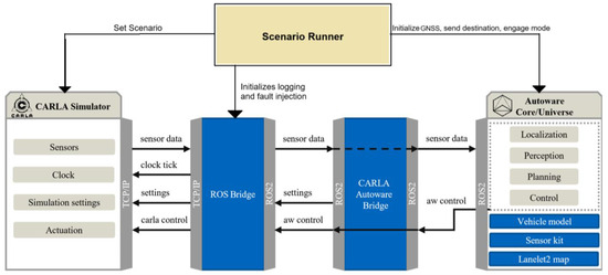
Figure 6.
CARLA Autoware modified bridge (based on [88]).
4.2. Scenario Runner Modifications
In order to efficiently test the resilience and the behavior of autonomous driving systems under various fault conditions, it is necessary to execute a test run multiple times. Manually configuring and executing each run is time-consuming and error-prone. To address this, we extended Scenario Runner to support automated batch execution of test runs. Each test run consists of a specific scenario (from the workload) combined with a fault configuration (from the faultload).
Additionally, since the ego vehicle is managed externally through the Autoware integration rather than by the CARLA Scenario Runner itself, we modified the Scenario Runner to detect and attach to a pre-existing ego vehicle within the simulation. This avoids redundant instantiation and enables compatibility with externally controlled systems.
During each test run, sensor data and safety-related events (e.g., collisions, lane invasions) are logged, enabling post-analysis of how different fault types affect the vehicle’s behavior. This automation improves reproducibility and expands test coverage while minimizing manual intervention.
4.3. Sensor Fault Injection System Implementation
The sensor fault injection framework is modular and extensible. It is centered around a base class named FaultInjector that attaches to the ROS bridge at the point where simulator sensor messages are converted into ROS topics. At this injection point, the framework alters the sensor streams before publication, so any ROS-based autonomous driving stack can be exercised without changing its internal modules. The system under test then consumes these topics as if they originated from malfunctioning sensors. In our case, the Autoware perception and localization modules read the modified data unchanged. The class diagram is presented in Figure 7.
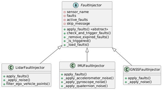
Figure 7.
Fault injector class diagram.
The framework was implemented in Python and integrated into the CARLA ROS bridge, which is built on ROS 2 Humble. It uses JSON configuration files, depends on CARLA’s Python API, and is compatible with Autoware.Universe.
Each sensor type, LiDAR, IMU, and GNSS, is handled by a dedicated subclass (LidarFaultInjector, IMUFaultInjector, and GNSSFaultInjector, respectively), all inheriting from the FaultInjector base class. This base class provides shared functionality, including fault management, activation logic, and the apply_faults() abstract method, which is implemented by each subclass. Although a camera sensor is included in our sensor configuration, no faults were injected into it, because it was not functional in the version of Autoware.Universe used in this work.
The FaultInjector class is tightly coupled with the Sensor class from the ROS bridge, which handles the conversion of CARLA sensor data to ROS 2 message formats. Upon initialization, FaultInjector loads a fault injection configuration file in JSON format. This configuration defines the location, type, trigger, and duration. Each time a new sensor message is received, the FaultInjector checks whether any faults should be applied, updates the list of active faults, and deactivates those whose duration has expired.
Two main fault types are supported: noise and silent failure. Noise is used to simulate degraded sensor output due to environmental or hardware-induced disturbances (e.g., electromagnetic interference, vibrations, or aging components). Silent failures represent cases in which a sensor stops sending data.
The LidarFaultInjector modifies the point cloud data by adding configurable Gaussian noise or stopping data publication to simulate a silent failure. Noise parameters (e.g., min_noise, max_noise) are defined in the JSON configuration file.
The IMUFaultInjector injects Gaussian noise independently into the gyroscope, accelerometer, and orientation quaternion data. It can also simulate silent failures for the entire IMU stream.
The GNSSFaultInjector applies noise to latitude, longitude, and altitude values and can simulate complete GNSS silent failures.
The fault injection configuration is sent by Scenario Runner as a JSON file and includes all necessary data, sensor (“LiDAR”, “IMU”, “GNSS”), faults (“noise” or “silent”), trigger (map-based location where the ego vehicle needs to be to trigger the fault), duration (time in seconds, 0 if permanent), and other parameters (fault-specific configuration, such as noise amplitude range). Figure 8 showcases an example of a sensor configuration file.
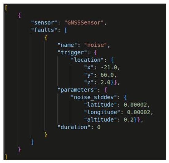
Figure 8.
Sensor Fault configuration example.
This design ensures that faults are applied in a consistent and reproducible manner relative to the scenario configuration and trigger conditions, making the system suitable for controlled experiments across multiple test runs.
The current implementation supports silent failure and severe noise for LiDAR, GNSS, and IMU. The same injection point in the ROS bridge allows additional fault models (constant bias/offset, drift as a random walk, stuck-at outputs, latency/jitter, and intermittent dropouts, among others) to be added with minimal changes, and to be applied to other sensors as the system under test and simulator interfaces permit. In this first iteration, we model “severe noise” as a zero-mean Gaussian, providing a basic way to perturb the sensors and offering a reproducible way to stress the AV stack without targeting a particular sensor’s physics [89]. While Gaussian noise is a useful baseline, real measurement errors are often non-Gaussian or time-correlated. For example, inertial sensors exhibit white noise plus bias instability/random walks [90], and GNSS errors in urban scenes show heavy-tailed residuals from multipath and blockage [91]. LiDAR in rain, fog, or snow [92] produces outliers and missing returns rather than purely Gaussian jitter.
4.4. Logging and Results Collection
ScenarioRunner provides mechanisms for collecting and exporting the results of each test run. Each scenario defines a set of relevant criteria by adding them to a behavior tree. This set determines what is monitored and what constitutes success or failure for that scenario, then the result for each criterion is stored in a file (txt, xml, or json). The criteria can be, collision (if the ego vehicle collided), route completion (how much of the planned route was completed), running redlight (detects if the ego vehicle ran a red light), Off road (if the vehicle left the drivable area), sidewalk (if the ego vehicle drove on the sidewalk), maximum route speed (if the vehicle did not surpass a certain velocity), and many more. The outcome is then calculated based on each criterion, and if all the criteria “Passed”, then the result is “Success”; otherwise, “Failure”.
5. Experimental Setup
This section describes the simulation environment, sensor configuration, fault model, and injection methodology used to assess the impact of sensor faults on autonomous vehicle behavior.
5.1. Simulation Environment and System Under Test
We distinguish between the simulation framework and the system under test. The framework comprises CARLA, the Scenario Runner orchestration, and the modified ROS bridge, where faults are injected and logs are recorded. The system under test is the Autoware-based autonomous driving stack used as the demonstration case. The framework delivers scenarios and perturbed sensor streams but does not implement perception, planning, or control logic. All observed behaviors, therefore, reflect the system under test and its configuration.
We used Town10 from CARLA’s map library as the simulation environment. This urban scenario offers a complex road network with multiple intersections, varied curvature, and diverse traffic conditions, making it suitable for testing sensor performance and autonomous decision-making under realistic conditions. To better match real-world traffic regulations and ensure consistency with map-based planning in Autoware, stop signs were manually added to the corresponding Lanelet2 map. This adjustment was necessary to reflect road rules that were not originally encoded in the base map and to trigger more meaningful behavior in the planning module.
The system under test follows the default TUMFTM sensor suite, which includes LiDAR, GNSS, and IMU. The camera was excluded because it was not functional in the Autoware version used, and the traffic light perception pipeline did not operate reliably, as it was constantly failing to recognize traffic lights; similar difficulties are reported in the Autoware issue tracker and CARLA–Autoware discussions. To avoid perception instability, we restricted the sensor configuration to LiDAR/GNSS/IMU for this study and left camera reintegration to future work [93,94]. No internal Autoware modules were modified and all parameters relevant to perception, localization, planning, and control were kept constant across runs. This configuration enables closed-loop interaction between CARLA and Autoware so that sensor-level faults can be injected at the framework layer and their effects on the behavior of the system under test can be observed.
5.2. Fault Model
We defined a fault model (or failure model, from the perspective of the sensor subsystems) characterized by the following four dimensions:
- Location—the location of the fault refers to the specific sensor affected. In this case, 5 different locations were considered: LiDAR, GNSS, and the three components of the IMU (gyroscope, accelerometer, and quaternion).
- Type—the fault type includes Silent Failures, where the sensor stops transmitting data, and noise, representing random deviations beyond the sensor’s normal operating conditions. We refer to this as Severe Noise.
- Trigger—the trigger defines the position where the ego vehicle must be to start the fault injection. We defined 5 fault triggers based on the moments the ego vehicle reaches specific locations within the map of the scenario.
- Duration—the duration of the fault specifies how long the fault remains active since the trigger. We defined a permanent duration, meaning the fault remains active until the end of the test run.
5.3. Severe Noise per Fault Location
In this section, we describe how the Severe Noise fault type was defined for each fault location, since different sensors behave in different ways. To define appropriate values for severe noise, we first identified the expected nominal noise levels for each sensor. These nominal values represent the typical measurement variability under normal operating conditions, as specified by manufacturers or reported in the literature. While such noise is always present in real-world deployments, it does not represent a fault. Instead, it serves as a reference baseline, helping us determine what constitutes abnormal or faulty behavior. Based on these nominal values, we established the corresponding severe noise levels used in our fault model.
5.3.1. LiDAR
To emulate noise in LiDAR data, we apply Gaussian noise to each point of the LiDAR point cloud. This fault represents small, random disturbances that real LiDAR sensors experience due to electronic interference, surface reflectivity, environmental conditions (e.g., dust, rain), or inherent sensor limitations [42,95,96].
The fault is implemented by adding a random noise to each coordinate (x, y, z) of every point in the cloud. The noise follows a Gaussian distribution centered around zero, meaning it introduces unbiased jitter around the true value. However, rather than focusing on absolute noise values (e.g., ±0.006 m), the significance of the fault is evaluated based on its relative deviation from the true point location.
Coordinate deviations up to 2% of the point’s range (distance from the sensor) are considered within expected tolerance for high-quality LiDARs. This value is consistent with findings in [97], which reported measurement errors within 1–2% for commercial terrestrial laser scanners operating under controlled conditions. Deviations between 2% and 10% are interpreted as severe deviations which translate into significant measurement corruption, likely leading to misperception, missed obstacles, or map inconsistencies. This percentage-based approach ensures that the added noise is significant, no matter the distance of the objects. For example, a 1 cm deviation is negligible for an object 50 m away but might completely distort a nearby point at 0.2 m. Furthermore, LiDAR returns are more sensitive at close range due to angular resolution and time-of-flight constraints, making small absolute changes more impactful.
By using this method, the simulation can capture both realistic sensor imperfections and fault-level disturbances, depending on the severity of the injected noise.
5.3.2. GNSS
To emulate positioning errors in a simulated autonomous system, we applied Gaussian noise to the GNSS readings, specifically affecting latitude, longitude, and altitude values. This type of fault replicates common disturbances encountered in real-world GNSS signals caused by atmospheric interference, satellite geometry (e.g., dilution of precision), multipath reflections, and receiver limitations [52,61,98].
A deviation of 0.00002 degrees both in latitude and longitude corresponds to approximately 2 m of horizontal error. The altitude noise was set to 0.2 m. These values align with the performance of single-frequency, civilian-grade GNSS receivers under open-sky conditions, where horizontal errors are typically under 3 m [99]. To emulate noise that exceeds nominal values, we adopted a standard deviation of 0.0002 degrees for latitude and longitude, corresponding to around 10 m of horizontal error. For altitude, a standard deviation of 2.0 m was defined. These values simulate degraded conditions due to poor satellite visibility, urban canyons, or intentional interference, which can degrade accuracy to over 10 m.
5.3.3. IMU
IMU faults are emulated by interfering separately with the following IMU measurements: angular velocity (gyroscope), linear acceleration (accelerometer), and orientation (quaternion). The purpose is to inject faults that are more severe than the natural variability and imperfections found in real-world IMUs due to mechanical, electronic, and environmental factors [98].
In commercial gyroscopes, bias instability and rate noise typically produce errors in the range of 0.01–0.05°/s, depending on environmental conditions and sampling rate. According to datasheet specifications, devices such as the Bosch BMI160 [100] or InvenSense MPU-6000 [101] show noise densities around 0.005–0.01°/s/√Hz. A 5% deviation threshold corresponds well to the upper bound of expected operating noise for angular velocity measurements under normal conditions. A deviation between 5 and 50% in gyroscopic output could indicate that the system is significantly misestimating rotational speed, leading to severe orientation estimation errors when fused with accelerometer and GNSS data.
Accelerometer nominal deviations are commonly expressed in µg/√Hz. For instance, the ADXL345 [102] shows typical deviation densities of ~150 µg/√Hz. For acceleration signals in the range of 1–2 m/s2 (e.g., steady cruising), a 5% deviation equates to ±0.05–0.1 m/s2, matching real-world fluctuations from road vibration or minor sensor inaccuracies. Noise values between 5 and 50% can seriously distort vehicle state estimation, especially when the signal-to-noise ratio is low, such as during smooth braking or slow turns.
Quaternions, derived from fused gyroscope and accelerometer data (and usually magnetometer), are sensitive to noise in both sensors [103]. Minor noise (<5%) can be expected due to integration drift or transient instability in attitude estimation filters. In simulation, this would translate to slight deviations in yaw, pitch, or roll, typical of nominal system behavior. Quaternion errors can simulate the effects of drift caused by improper sensor fusion or misalignment in orientation. This can lead to cascading failures in localization and control if not properly corrected. A distortion between 5 and 50% in quaternion values is equivalent to a significant misestimation of heading or tilt.
5.3.4. Summary of Fault Type Values per Location
This section summarizes the fault injection parameters used to emulate Severe Noise conditions in the different sensors, as well as presenting the nominal values, i.e., the noise that naturally occurs in every sensor, according to its specifications. Table 1 presents a structured overview of the Nominal values and the Severe Noise values per sensor.

Table 1.
Summary of noise values used in fault model.
5.4. Fault Trigger
The experimental campaign is structured around a driving scenario designed in the CARLA simulator using the Town10 map. This scenario reflects a typical urban driving situation in which the autonomous system must operate safely under varying conditions. Sensor faults were introduced at strategic points to assess the vehicle’s behavior under different conditions of the AV and the surrounding environment. The ego vehicle used in all scenarios is a green van being controlled by Autoware.Universe version 2019.1.
Traffic lights present in the simulation environment were not considered, as the specific version of Autoware.Universe traffic light detection was not working. Therefore, vehicle behavior at intersections was governed solely by map-based rules, stop signs, and dynamic interactions with other road users.
As seen in Figure 9, the yellow line represents the route that the vehicle takes, and each blue point is a fault injection trigger.
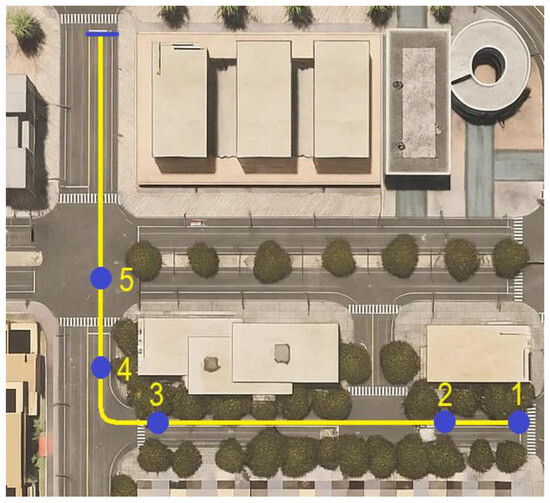
Figure 9.
Scenarios Route.
By organizing the experiments into these five fault triggers, the testing framework captures a diverse set of real-world driving events and enables a detailed analysis of sensor fault impacts across multiple autonomous vehicle functions.
5.4.1. Trigger 1: Starting Point
The vehicle begins its route on a straight road, requiring accurate lane keeping and localization. This initial phase occurs before reaching any traffic control elements and serves to validate basic navigation, localization, and sensor fusion during nominal driving. Sensor faults introduced here test the system’s ability to maintain a stable trajectory in the absence of external constraints or decision points.
5.4.2. Trigger 2: Stop Sign
The vehicle approaches a stop sign and is required to halt and yield to a passing vehicle, and then it should wait for cross-traffic before proceeding. This scenario focuses on evaluating stop accuracy, map-based rule adherence, and cross-traffic awareness during controlled deceleration [104,105].
5.4.3. Trigger 3: Right Turn at Intersection
The vehicle must execute a right turn at a T-junction. This maneuver tests the system’s lateral control and path-following capabilities while navigating curved trajectories near road edges and potential obstacles [104,105,106].
5.4.4. Trigger 4: Pedestrian Crosswalk Encounter
At this point (see also Figure 10), the ego vehicle approaches a marked pedestrian crosswalk. A pedestrian actor is programmed to cross the street from the right side of the road as the ego vehicle nears the crosswalk. The objective is to evaluate the AV’s perception and decision-making capabilities in response to dynamic pedestrian activity. The vehicle is expected to detect the pedestrian in advance, decelerate appropriately, and yield before the crossing zone. Sensor faults in this segment primarily challenge the detection of small and moving objects. Notably, faults affecting the LiDAR or camera may reduce detection confidence, while IMU or GNSS faults can affect precise positioning near the stop line.
Figure 10.
Fourth Trigger.
5.4.5. Trigger 5: Final Intersection
In the final scenario, the vehicle reaches an intersection with no traffic signals, requiring it to yield to vehicles coming from the right. This situation stresses the vehicle’s ability to assess right-of-way and respond correctly under partial perception failures.
5.5. Results Classification
To assess overall experiment results, we classify the vehicle’s behavior on each fault injection run into four categories:
- Collision: The ego vehicle collides with another object, pedestrian, or road infrastructure.
- Out: The vehicle deviates from its designated lane or route but does not collide.
- Timeout: The vehicle fails to reach the destination within the time limit (3 min). It probably stopped, but did not collide or deviate from the designated lane or route
- OK: The vehicle completes the route without any incident.
The fault is tolerated only if the outcome of the run is OK, meaning that the mission was successfully accomplished, despite the injected fault. A Timeout means the fault was not tolerated, but the vehicle failed safely (no harm was done, i.e., no collision, nor lane/route departure). Out and Collision outcomes are both severe failures, since they can potentially result in harm to people, damage to the environment, or major loss of property.
5.6. Fault Injection Process
A fault injection experiment consists of a series of test runs, each injecting a single fault, according to its location, type, trigger and duration.
A test runner iterates through the list of fault configurations, executing a separate test run for each one. After the test run, the outcomes—such as collisions, route completion, or traffic rule violations—are logged into a file for later analysis and results classification. The simulation environment (CARLA and Autoware) is then reset, the ego vehicle is positioned at the start, the scenario is loaded, and the ego vehicle is started, launching the next test run. This ensures that every test begins in a consistent initial state, supporting structured and reproducible tests under the same initial conditions.
5.7. Experimental Setup Validation Process
All experiments run in synchronous simulation. We log simulation time and all the messages across repeated runs and confirm that these traces are consistent. With the injection disabled, we also capture the same ROS topics immediately before and after the injection interface in the bridge and verify that payloads and message rates are identical.
We then execute test runs with only nominal sensor noise. In these golden runs, the system under test completes the scenario without incidents, which indicates that the framework does not introduce unintended disturbances. Repeating the golden runs yields the same outcome, which provides a reproducibility baseline for our experiments.
For the faults used in this study, we verify the expected signal effects at the injection point. For silent failure, the post-injection topic rate drops to zero at activation and remains at zero until the end of the run. For severe noise, the post-injection stream shows the variance increase configured for each location. Activation occurs when the ego vehicle reaches the route positions and logs the trigger identifier and timestamps. The fault duration is permanent until the end of each run.
These procedures demonstrate the operational validity of the experimental infrastructure in nominal mode and the correct application of the faults for our scenarios. They are not an exhaustive validation across all sensors, fault types, or environments.
6. Experimental Execution and Results
This section presents the fault injection experimental results and analyzes the observed outcomes.
6.1. Golden Runs
To validate the experimental setup and ensure the correct functioning of the system under normal conditions, a series of test runs was executed, where the fault injection mechanism was used to introduce disturbances in the sensor readings, below the Nominal value limits (see Table 1). These tests are called Golden Runs, and serve two primary purposes: (1) to verify the correct functioning of the AV under typical sensor noise conditions, and (2) to validate the fault injection mechanism by confirming that it does not interfere with the expected system behavior in the absence of actual faults.
An experimental campaign with 25 test runs was executed, introducing Nominal noise in each of the 5 locations, at each of the 5 Triggers. The results can be seen in Table 2, confirming that the system behaved as expected since Autoware completed each run without safety violations, route deviations, or abnormal behavior.
Table 2.
Golden run results.
6.2. Experiment Execution and Analysis
Following the Golden Runs, the fault injection experiment was executed in a fully automated and repeatable manner. A total of 50 fault injection runs were executed, consisting of a combination of the 5 different Fault Locations (GNSS, LiDAR, IMU gyroscope, IMU accelerometer, and IMU quaternion), two fault types (Silent Failure and Severe Noise), and five injection triggers (Trigger 1 to Trigger 5). The use of these structured dimensions ensured consistency and coverage across relevant sensor failure modes and situations. Table 3 summarizes the results and provides an overall view of the results obtained by fault location, type, and trigger.
Table 3.
Test run results.
At a glance, the analysis of these 50 test runs revealed patterns in how the applied faults affected the AV’s behavior.
Regarding GNSS, the tested Autoware configuration showed resilience across all fault scenarios. Whether subjected to silent sensor failures or severe noise, Autoware reliably maintained accurate localization and safe navigation. This is expected for the tested stack, in which pose is produced by NDT LiDAR–map registration and an EKF that fuses IMU and GNSS, which effectively compensate for GNSS inaccuracies or signal loss. In our urban route, LiDAR–map updates dominated the pose estimate, while GNSS acted as an initializer/low-authority absolute aid. Perturbing GNSS, therefore, did not change behavior in these scenarios. This should not be read as a general claim that GNSS is unimportant, since on open highways or in feature-poor areas, GNSS can have greater influence; however, the scenario used in this study does not cover this case.
The tested configuration maintained stable control and accurate localization in all IMU accelerometer failures, including severe noise. With LiDAR–map pose updates anchoring the filter, accelerometer disturbances were down-weighted by the EKF and did not produce observable effects in these scenarios.
IMU Quaternion perturbations were absorbed without incident. With yaw dynamics driven primarily by the gyroscope and pose regularly corrected by LiDAR–map matching, moderate orientation noise in the fused quaternion did not destabilize planning or control in our runs.
The LiDAR sensor failure results revealed critical weaknesses in the tested Autoware configuration design. Silent sensor failures (complete loss of LiDAR data) consistently led to immediate and severe failures, since the vehicle kept driving until colliding with other vehicles or pedestrians. On the other hand, Severe Noise LiDAR disturbances systematically stopped the car, leading to test timeouts, indicating Autoware’s reliance on LiDAR-based perception and its limited capacity to effectively handle significant sensor degradation. However, no collision occurred, revealing fail-safe behavior from the system. This reflects the tested stack’s reliance on LiDAR for both perception and LiDAR–map localization. When the LiDAR signal is removed, the system loses its primary pose/perception source, whereas strong degradation triggers fail-safe behavior.
Analyzing the IMU gyroscope results, the autonomous vehicle demonstrated strong resilience against silent sensor failures, consistently completing all scenarios successfully. However, under severe noise conditions of the IMU gyroscope, the tested AV stack revealed significant vulnerabilities, producing erratic vehicle movements characterized by lateral instability. Silent sensor failure is tolerated because NDT provides frequent pose/yaw corrections and the EKF ignores missing measurements. However, noisy yaw-rate is more harmful because it injects the wrong heading between NDT updates. These severe disturbances frequently resulted in unsafe outcomes, such as collisions with pedestrians or obstacles, deviations from lane, and timeouts due to the vehicle’s inability to effectively plan or execute stable trajectories. To ensure data validity, additional tests were conducted in cases involving severe noise on the IMU gyroscope, with five extra runs performed for each trigger to account for the variability in vehicle behavior.
The repeated tests, shown in Table 4, further confirmed this instability, emphasizing the critical role of angular velocity information provided by the gyroscope for safe navigation and stable control of the vehicle. These results highlight the need for enhancing Autoware’s fault detection mechanisms and redundancy strategies, specifically targeting the gyroscope’s angular velocity data.
Table 4.
Additional gyroscope test results.
In summary, the results of this experimental campaign provide clear guidance regarding the criticality and resilience of each sensor within Autoware’s autonomous driving stack. The gyroscope and LiDAR sensors are particularly vulnerable to severe fault conditions, necessitating targeted improvements in fault detection, redundancy mechanisms, and enhanced fallback strategies. However, the accelerometer, quaternion orientation, and GNSS sensors demonstrated notable resilience, effectively handled by Autoware’s existing sensor fusion methodologies. These insights lay a foundation for future research directions, specifically aiming to reinforce the autonomous system’s fault tolerance and overall safety performance under realistic sensor failure conditions.
The full list of tests, including the golden runs, is listed in Table A1.
7. Conclusions and Future Work
This work presented a fault injection framework combining the CARLA simulator with the Autoware autonomous driving stack to explore how autonomous vehicles behave under different types of sensor anomalies. The framework was used to conduct targeted experiments involving silent sensor failures and severe noise across key sensors such as LiDAR, GNSS, and components of the inertial measurement unit, including gyroscope, accelerometer, and quaternion. The purpose was to enable the simulation of adverse sensing conditions and to observe and analyze system behavior during such events.
The experimental results obtained using our framework highlight its potential, revealing insights into how the autonomous driving system responds to various sensor faults. The framework allowed us to identify critical situations where specific sensor failures, such as severe LiDAR noise or silent faults, consistently led to hazardous outcomes like collisions or navigation failures. These observations suggest a strong system dependence on certain sensors, such as LiDAR for perception and the IMU gyroscope for orientation stability. In contrast, other sensors, such as GNSS, the IMU accelerometer, and the quaternion components, showed higher fault tolerance under similar conditions. While these findings helped uncover potential vulnerabilities in Autoware’s current implementation, the primary contribution lies in demonstrating how the proposed fault injection framework can support the assessment of sensor resilience in autonomous systems.
The results in this study were obtained entirely in simulation using CARLA and Autoware as the system under test. Although modern simulators provide realistic environments and sensor models, they cannot fully capture real-world complexity. Important gaps include sensor artifacts such as contamination, electromagnetic interference, and hardware aging, as well as the influence of human and traffic interactions that shape safety outcomes in practice. Accordingly, the findings should be read as relative indicators of system resilience in a controlled setting rather than definitive on road performance. For future work, we plan to compare outcomes against data from physical experiments and public datasets that contain real sensor faults, for example, datasets that capture LiDAR degradation [107] and the ROD2021 radar dataset [108], to improve model fidelity and assess the transferability of results to real vehicles.
Future research directions include extending the fault injection framework to additional faults, such as intermittent sensor failures, calibration errors, and gradual sensor drift. Evaluating alternative AV software stacks, such as Apollo, would facilitate broader validation of results and a deeper understanding of system-specific resilience. Moreover, integrating real-time fault detection and diagnosis modules into the simulation environment would support proactive fault management, enhancing autonomous driving systems’ safety and reliability. Finally, future work should focus on instrumenting internal components of the AV software stack, such as the controller and decision-making modules, to better understand system behavior under faulty conditions. This would not only allow researchers to observe the system’s global response but also enable detailed analysis of how faults propagate through individual modules and contribute to failures. Alternatively, we can also focus on assessing portability to OEM architectures by prototyping a ROS 2—SOME/IP gateway and an AUTOSAR-native injector that perturbs ara::com sensor services, leveraging the ASIRA interoperability pattern, so that the framework can be used with Adaptive AUTOSAR stacks.
Author Contributions
Conceptualization, J.C. and J.D.; Methodology, F.M., J.C. and J.D.; Software, F.M.; Validation, F.M., J.C. and J.D.; Formal analysis, F.M., J.C. and J.D.; Investigation, F.M.; Resources, F.M.; Data curation, F.M.; Writing—original draft preparation, F.M.; Writing—review and editing, F.M., J.C. and J.D.; Supervision, J.C. and J.D.; Project administration, J.C. and J.D.; Funding acquisition, J.C. All authors have read and agreed to the published version of the manuscript.
Funding
This research received no external funding.
Data Availability Statement
Data is contained within the article.
Acknowledgments
During the preparation of this manuscript, the authors used ChatGPT (GPT-4, OpenAI) for text checking and figure adjustments. The authors have reviewed and edited the output thoroughly and take full responsibility for the content of this publication.
Conflicts of Interest
The authors declare no conflicts of interest.
Abbreviations
The following abbreviations are used in this manuscript:
| AD | Autonomous Driving |
| ADS | Autonomous Driving System |
| AI | Artificial Intelligence |
| API | Application Programming Interface |
| AV | Autonomous Vehicle |
| AVFI | Autonomous Vehicle Fault Injection |
| CARLA | Car Learning to Act (Simulator) |
| CPU | Central Processing Unit |
| CVC | Computer Vision Center |
| DVS | Dynamic Vision Sensor |
| FMCW | Frequency-Modulated Continuous Wave |
| GNSS | Global Navigation Satellite System |
| GPS | Global Positioning System |
| HMI | Human–Machine Interface |
| IMU | Inertial Measurement Unit |
| INS | Inertial Navigation System |
| IP | Internet Protocol |
| ISO | International Organization for Standardization |
| JSON | JavaScript Object Notation |
| LGSVL | LG Simulator for Autonomous Vehicles |
| MPU | Microprocessor Unit |
| NDT | Normal Distributions Transform |
| RADAR | Radio Detection and Ranging |
| RGB | Red Green Blue (color model) |
| ROS | Robot Operating System |
| SLAM | Simultaneous Localization and Mapping |
| TCP | Transmission Control Protocol |
| WGS | World Geodetic System |
| XML | eXtensible Markup Language |
Appendix A
Table A1.
Full list of Fault Injection results.
Table A1.
Full list of Fault Injection results.
| Fault ID | Location | Type | Trigger | Outcome |
|---|---|---|---|---|
| 1 | IMU—Gyroscope | Silent | Scenario 1 | OK |
| 2 | IMU—Gyroscope | Silent | Scenario 2 | OK |
| 3 | IMU—Gyroscope | Silent | Scenario 3 | OK |
| 4 | IMU—Gyroscope | Silent | Scenario 4 | OK |
| 5 | IMU—Gyroscope | Silent | Scenario 5 | OK |
| 6 | IMU—Gyroscope | Noise | Scenario 1 | OK |
| 7 | IMU—Gyroscope | Noise | Scenario 2 | OK |
| 8 | IMU—Gyroscope | Noise | Scenario 3 | OK |
| 9 | IMU—Gyroscope | Noise | Scenario 4 | OK |
| 10 | IMU—Gyroscope | Noise | Scenario 5 | OK |
| 11 | IMU—Gyroscope | Severe | Scenario 1 | Collision |
| 12 | IMU—Gyroscope | Severe | Scenario 2 | Collision |
| 13 | IMU—Gyroscope | Severe | Scenario 3 | Timeout |
| 14 | IMU—Gyroscope | Severe | Scenario 4 | Collision |
| 15 | IMU—Gyroscope | Severe | Scenario 5 | Out |
| 16 | IMU—Accelerometer | Silent | Scenario 1 | OK |
| 17 | IMU—Accelerometer | Silent | Scenario 2 | OK |
| 18 | IMU—Accelerometer | Silent | Scenario 3 | OK |
| 19 | IMU—Accelerometer | Silent | Scenario 4 | OK |
| 20 | IMU—Accelerometer | Silent | Scenario 5 | OK |
| 21 | IMU—Accelerometer | Noise | Scenario 1 | OK |
| 22 | IMU—Accelerometer | Noise | Scenario 2 | OK |
| 23 | IMU—Accelerometer | Noise | Scenario 3 | OK |
| 24 | IMU—Accelerometer | Noise | Scenario 4 | OK |
| 25 | IMU—Accelerometer | Noise | Scenario 5 | OK |
| 26 | IMU—Accelerometer | Severe | Scenario 1 | OK |
| 27 | IMU—Accelerometer | Severe | Scenario 2 | OK |
| 28 | IMU—Accelerometer | Severe | Scenario 3 | OK |
| 29 | IMU—Accelerometer | Severe | Scenario 4 | OK |
| 30 | IMU—Accelerometer | Severe | Scenario 5 | OK |
| 31 | IMU—Quaternion | Silent | Scenario 1 | OK |
| 32 | IMU—Quaternion | Silent | Scenario 2 | OK |
| 33 | IMU—Quaternion | Silent | Scenario 3 | OK |
| 34 | IMU—Quaternion | Silent | Scenario 4 | OK |
| 35 | IMU—Quaternion | Silent | Scenario 5 | OK |
| 36 | IMU—Quaternion | Noise | Scenario 1 | OK |
| 37 | IMU—Quaternion | Noise | Scenario 2 | OK |
| 38 | IMU—Quaternion | Noise | Scenario 3 | OK |
| 39 | IMU—Quaternion | Noise | Scenario 4 | OK |
| 40 | IMU—Quaternion | Noise | Scenario 5 | OK |
| 41 | IMU—Quaternion | Severe | Scenario 1 | OK |
| 42 | IMU—Quaternion | Severe | Scenario 2 | OK |
| 43 | IMU—Quaternion | Severe | Scenario 3 | OK |
| 44 | IMU—Quaternion | Severe | Scenario 4 | OK |
| 45 | IMU—Quaternion | Severe | Scenario 5 | OK |
| 46 | LiDAR | Silent | Scenario 1 | Collision |
| 47 | LiDAR | Silent | Scenario 2 | Collision |
| 48 | LiDAR | Silent | Scenario 3 | Collision |
| 49 | LiDAR | Silent | Scenario 4 | Collision |
| 50 | LiDAR | Silent | Scenario 5 | Collision |
| 51 | LiDAR | Noise | Scenario 1 | OK |
| 52 | LiDAR | Noise | Scenario 2 | OK |
| 53 | LiDAR | Noise | Scenario 3 | OK |
| 54 | LiDAR | Noise | Scenario 4 | OK |
| 55 | LiDAR | Noise | Scenario 5 | OK |
| 56 | LiDAR | Severe | Scenario 1 | Timeout |
| 57 | LiDAR | Severe | Scenario 2 | Timeout |
| 58 | LiDAR | Severe | Scenario 3 | Timeout |
| 59 | LiDAR | Severe | Scenario 4 | Timeout |
| 60 | LiDAR | Severe | Scenario 5 | Timeout |
| 61 | GNSS | Silent | Scenario 1 | OK |
| 62 | GNSS | Silent | Scenario 2 | OK |
| 63 | GNSS | Silent | Scenario 3 | OK |
| 64 | GNSS | Silent | Scenario 4 | OK |
| 65 | GNSS | Silent | Scenario 5 | OK |
| 66 | GNSS | Noise | Scenario 1 | OK |
| 67 | GNSS | Noise | Scenario 2 | OK |
| 68 | GNSS | Noise | Scenario 3 | OK |
| 69 | GNSS | Noise | Scenario 4 | OK |
| 70 | GNSS | Noise | Scenario 5 | OK |
| 71 | GNSS | Severe | Scenario 1 | OK |
| 72 | GNSS | Severe | Scenario 2 | OK |
| 73 | GNSS | Severe | Scenario 3 | OK |
| 74 | GNSS | Severe | Scenario 4 | OK |
| 75 | GNSS | Severe | Scenario 5 | OK |
| 76 | IMU—Gyroscope | Severe | Scenario 1 | Timeout |
| 77 | IMU—Gyroscope | Severe | Scenario 1 | Collision |
| 78 | IMU—Gyroscope | Severe | Scenario 1 | Out |
| 79 | IMU—Gyroscope | Severe | Scenario 1 | Collision |
| 80 | IMU—Gyroscope | Severe | Scenario 1 | Collision |
| 81 | IMU—Gyroscope | Severe | Scenario 2 | Out |
| 82 | IMU—Gyroscope | Severe | Scenario 2 | Collision |
| 83 | IMU—Gyroscope | Severe | Scenario 2 | Collision |
| 84 | IMU—Gyroscope | Severe | Scenario 2 | Collision |
| 85 | IMU—Gyroscope | Severe | Scenario 2 | Timeout |
| 86 | IMU—Gyroscope | Severe | Scenario 3 | Out |
| 87 | IMU—Gyroscope | Severe | Scenario 3 | Collision |
| 88 | IMU—Gyroscope | Severe | Scenario 3 | Out |
| 89 | IMU—Gyroscope | Severe | Scenario 3 | Collision |
| 90 | IMU—Gyroscope | Severe | Scenario 3 | Collision |
| 91 | IMU—Gyroscope | Severe | Scenario 4 | Collision |
| 92 | IMU—Gyroscope | Severe | Scenario 4 | Timeout |
| 93 | IMU—Gyroscope | Severe | Scenario 4 | Collision |
| 94 | IMU—Gyroscope | Severe | Scenario 4 | Collision |
| 95 | IMU—Gyroscope | Severe | Scenario 4 | Timeout |
| 96 | IMU—Gyroscope | Severe | Scenario 5 | Collision |
| 97 | IMU—Gyroscope | Severe | Scenario 5 | Collision |
| 98 | IMU—Gyroscope | Severe | Scenario 5 | Timeout |
| 99 | IMU—Gyroscope | Severe | Scenario 5 | Timeout |
| 100 | IMU—Gyroscope | Severe | Scenario 5 | Out |
References
- Silva, Ó.; Cordera, R.; González-González, E.; Nogués, S. Environmental impacts of autonomous vehicles: A review of the scientific literature. Sci. Total Environ. 2022, 830, 154615. [Google Scholar] [CrossRef]
- Luca, O.; Andrei, L.; Iacoboaea, C.; Gaman, F. Unveiling the Hidden Effects of Automated Vehicles on “Do No Significant Harm’’ Components. Sustainability 2023, 15, 11265. [Google Scholar] [CrossRef]
- Ahangar, M.N.; Ahmed, Q.Z.; Khan, F.A.; Hafeez, M. A Survey of Autonomous Vehicles: Enabling Communication Technologies and Challenges. Sensors 2021, 21, 706. [Google Scholar] [CrossRef]
- Pandharipande, A.; Cheng, C.-H.; Dauwels, J.; Gurbuz, S.Z.; Ibanez-Guzman, J.; Li, G.; Piazzoni, A.; Wang, P.; Santra, A. Sensing and Machine Learning for Automotive Perception: A Review. IEEE Sens. J. 2023, 23, 11097–11115. [Google Scholar] [CrossRef]
- Jha, S.; Banerjee, S.S.; Cyriac, J.; Kalbarczyk, Z.T.; Iyer, R.K. AVFI: Fault Injection for Autonomous Vehicles. In Proceedings of the 48th Annual IEEE/IFIP International Conference on Dependable Systems and Networks Workshops, DSN-W 2018, Luxembourg, 25–28 June 2018; pp. 55–56. [Google Scholar] [CrossRef]
- Maleki, M.; Farooqui, A.; Sangchoolie, B. CarFASE: A Carla-based Tool for Evaluating the Effects of Faults and Attacks on Autonomous Driving Stacks. In Proceedings of the 53rd Annual IEEE/IFIP International Conference on Dependable Systems and Networks Workshops, DSN-W 2023, Porto, Portugal, 27–30 June 2023; pp. 92–99. [Google Scholar] [CrossRef]
- Jha, S.; Banerjee, S.; Tsai, T.; Hari, S.K.S.; Sullivan, M.B.; Kalbarczyk, Z.T.; Keckler, S.W.; Iyer, R.K. ML-Based Fault Injection for Autonomous Vehicles: A Case for Bayesian Fault Injection. In Proceedings of the 2019 49th Annual IEEE/IFIP International Conference on Dependable Systems and Networks (DSN), Portland, OR, USA, 24–27 June 2019; pp. 112–124. [Google Scholar] [CrossRef]
- Maleki, M.; Sangchoolie, B. SUFI: A Simulation-based Fault Injection Tool for Safety Evaluation of Advanced Driver Assistance Systems Modelled in SUMO. In Proceedings of the 2021 17th European Dependable Computing Conference, EDCC 2021, Munich, Germany, 13–16 September 2021; pp. 45–52. [Google Scholar] [CrossRef]
- Saraoglu, M.; Morozov, A.; Janschek, K. MOBATSim: MOdel-Based Autonomous Traffic Simulation Framework for Fault-Error-Failure Chain Analysis. IFAC-PapersOnLine 2019, 52, 239–244. [Google Scholar] [CrossRef]
- Gosavi, M.A.; Rhoades, B.B.; Conrad, J.M. Application of Functional Safety in Autonomous Vehicles Using ISO 26262 Standard: A Survey. In Proceedings of the IEEE SOUTHEASTCON 2018, St. Petersburg, FL, USA, 19–22 April 2018. [Google Scholar] [CrossRef]
- Gat, E.; Bonnasso, R.P.; Murphy, R. On Three-Layer Architectures. Artif. Intell. Mob. Robot. 1998, 195, 210. [Google Scholar]
- Subsumption Control of a Mobile Robot. Available online: https://www.researchgate.net/publication/2875073_Subsumption_Control_of_a_Mobile_Robot (accessed on 14 August 2025).
- The 3T Intelligent Control Architecture|Download Scientific Diagram. Available online: https://www.researchgate.net/figure/The-3T-Intelligent-Control-Architecture_fig1_2851637 (accessed on 14 August 2025).
- Iovino, M.; Scukins, E.; Styrud, J.; Ögren, P.; Smith, C. A survey of Behavior Trees in robotics and AI. Rob. Auton. Syst. 2022, 154, 104096. [Google Scholar] [CrossRef]
- García, C.E.; Prett, D.M.; Morari, M. Model predictive control: Theory and practice—A survey. Automatica 1989, 25, 335–348. [Google Scholar] [CrossRef]
- Pendleton, S.D.; Andersen, H.; Du, X.; Shen, X.; Meghjani, M.; Eng, Y.H.; Rus, D.; Ang, M.H. Perception, Planning, Control, and Coordination for Autonomous Vehicles. Machines 2017, 5, 6. [Google Scholar] [CrossRef]
- Velasco-Hernandez, G.; Yeong, D.J.; Barry, J.; Walsh, J. Autonomous Driving Architectures, Perception and Data Fusion: A Review. In Proceedings of the 2020 IEEE 16th International Conference on Intelligent Computer Communication and Processing (ICCP), Cluj-Napoca, Romania, 3–5 September 2020; pp. 315–321. [Google Scholar]
- Kumar, D.; Muhammad, N. A Survey on Localization for Autonomous Vehicles. IEEE Access 2023, 11, 115865–115883. [Google Scholar] [CrossRef]
- Chalvatzaras, A.; Pratikakis, I.; Amanatiadis, A.A. A Survey on Map-Based Localization Techniques for Autonomous Vehicles. IEEE Trans. Intell. Veh. 2023, 8, 1574–1596. [Google Scholar] [CrossRef]
- Karle, P.; Geisslinger, M.; Betz, J.; Lienkamp, M. Scenario Understanding and Motion Prediction for Autonomous Vehicles—Review and Comparison. IEEE Trans. Intell. Transp. Syst. 2022, 23, 16962–16982. [Google Scholar] [CrossRef]
- Wang, X.; Maleki, M.A.; Azhar, M.W.; Trancoso, P. Moving Forward: A Review of Autonomous Driving Software and Hardware Systems. arXiv 2024, arXiv:2411.10291. [Google Scholar] [CrossRef]
- He, Z.; Nie, L.; Yin, Z.; Huang, S. A Two-Layer Controller for Lateral Path Tracking Control of Autonomous Vehicles. Sensors 2020, 20, 3689. [Google Scholar] [CrossRef]
- Chen, G.; Zhao, X.; Gao, Z.; Hua, M. Dynamic Drifting Control for General Path Tracking of Autonomous Vehicles. IEEE Trans. Intell. Veh. 2023, 8, 2527–2537. [Google Scholar] [CrossRef]
- Yeong, D.J.; Velasco-Hernandez, G.; Barry, J.; Walsh, J. Sensor and Sensor Fusion Technology in Autonomous Vehicles: A Review. Sensors 2021, 21, 2140. [Google Scholar] [CrossRef]
- Ignatious, H.A.; Sayed, H.-E.; Khan, M. An overview of sensors in Autonomous Vehicles. Procedia Comput. Sci. 2022, 198, 736–741. [Google Scholar] [CrossRef]
- Matos, F.; Bernardino, J.; Durães, J.; Cunha, J. A Survey on Sensor Failures in Autonomous Vehicles: Challenges and Solutions. Sensors 2024, 24, 5108. [Google Scholar] [CrossRef]
- Ortiz, F.M.; Sammarco, M.; Costa, L.H.M.K.; Detyniecki, M. Applications and Services Using Vehicular Exteroceptive Sensors: A Survey. IEEE Trans. Intell. Veh. 2023, 8, 949–969. [Google Scholar] [CrossRef]
- Budisusila, E.N.; Khosyi’in, M.; Prasetyowati, S.A.D.; Suprapto, B.Y.; Nawawi, Z. Ultrasonic Multi-Sensor Detection Patterns on Autonomous Vehicles Using Data Stream Method. In Proceedings of the 2021 8th International Conference on Electrical Engineering, Computer Science and Informatics (EECSI), Semarang, Indonesia, 20–21 October 2021; pp. 144–150. [Google Scholar]
- Paidi, V.; Fleyeh, H.; Håkansson, J.; Nyberg, R.G. Smart parking sensors, technologies and applications for open parking lots: A review. IET Intell. Transp. Syst. 2018, 12, 735–741. [Google Scholar] [CrossRef]
- Vargas, J.; Alsweiss, S.; Toker, O.; Razdan, R.; Santos, J. An Overview of Autonomous Vehicles Sensors and Their Vulnerability to Weather Conditions. Sensors 2021, 21, 5397. [Google Scholar] [CrossRef] [PubMed]
- Rosique, F.; Navarro, P.J.; Fernández, C.; Padilla, A. A Systematic Review of Perception System and Simulators for Autonomous Vehicles Research. Sensors 2019, 19, 648. [Google Scholar] [CrossRef]
- Wang, Z.; Wu, Y.; Niu, Q. Multi-Sensor Fusion in Automated Driving: A Survey. IEEE Access 2020, 8, 2847–2868. [Google Scholar] [CrossRef]
- Komissarov, R.; Kozlov, V.; Filonov, D.; Ginzburg, P. Partially coherent radar unties range resolution from bandwidth limitations. Nat. Commun. 2019, 10, 1423. [Google Scholar] [CrossRef]
- Skaria, S.; Al-Hourani, A.; Evans, R.J.; Sithamparanathan, K.; Parampalli, U. Interference Mitigation in Automotive Radars Using Pseudo-Random Cyclic Orthogonal Sequences. Sensors 2019, 19, 4459. [Google Scholar] [CrossRef]
- Pirkani, A.; Norouzian, F.; Hoare, E.; Cherniakov, M.; Gashinova, M. Automotive interference statistics and their effect on radar detector. IET Radar Sonar Navig. 2022, 16, 9–21. [Google Scholar] [CrossRef]
- Wu, Z.; Song, Y.; Liu, J.; Chen, Y.; Sha, H.; Shi, M.; Zhang, H.; Qin, L.; Liang, L.; Jia, P.; et al. Advancements in Key Parameters of Frequency-Modulated Continuous-Wave Light Detection and Ranging: A Research Review. Appl. Sci. 2024, 14, 7810. [Google Scholar] [CrossRef]
- Staffas, T.; Elshaari, A.; Zwiller, V. Frequency modulated continuous wave and time of flight LIDAR with single photons: A comparison. Opt. Express 2024, 32, 7332–7341. [Google Scholar] [CrossRef]
- Ma, J.; Zhuo, S.; Qiu, L.; Gao, Y.; Wu, Y.; Zhong, M.; Bai, R.; Sun, M.; Chiang, P.Y.; Ma, J.; et al. A review of ToF-based LiDAR. J. Semicond. 2024, 45, 101201. [Google Scholar] [CrossRef]
- Li, N.; Ho, C.P.; Xue, J.; Lim, L.W.; Chen, G.; Fu, Y.H.; Lee, L.Y.T. A Progress Review on Solid-State LiDAR and Nanophotonics-Based LiDAR Sensors. Laser Photon Rev. 2022, 16, 2100511. [Google Scholar] [CrossRef]
- Holzhüter, H.; Bödewadt, J.; Bayesteh, S.; Aschinger, A.; Blume, H. Technical concepts of automotive LiDAR sensors: A review. Opt. Eng. 2023, 62, 031213. [Google Scholar] [CrossRef]
- Li, Y.; Ibanez-Guzman, J. Lidar for Autonomous Driving: The Principles, Challenges, and Trends for Automotive Lidar and Perception Systems. IEEE Signal Process. Mag. 2020, 37, 50–61. [Google Scholar] [CrossRef]
- Dreissig, M.; Scheuble, D.; Piewak, F.; Boedecker, J. Survey on LiDAR Perception in Adverse Weather Conditions. In Proceedings of the 2023 IEEE Intelligent Vehicles Symposium (IV), Anchorage, AK, USA, 4–7 June 2023; pp. 1–8. [Google Scholar]
- Damodaran, D.; Mozaffari, S.; Alirezaee, S.; Ahamed, M.J. Experimental Analysis of the Behavior of Mirror-like Objects in LiDAR-Based Robot Navigation. Appl. Sci. 2023, 13, 2908. [Google Scholar] [CrossRef]
- Roszyk, K.; Nowicki, M.R.; Skrzypczyński, P. Adopting the YOLOv4 Architecture for Low-Latency Multispectral Pedestrian Detection in Autonomous Driving. Sensors 2022, 22, 1082. [Google Scholar] [CrossRef]
- Sun, C.; Chen, Y.; Qiu, X.; Li, R.; You, L. MRD-YOLO: A Multispectral Object Detection Algorithm for Complex Road Scenes. Sensors 2024, 24, 3222. [Google Scholar] [CrossRef]
- Xie, Y.; Zhang, L.; Yu, X.; Xie, W. YOLO-MS: Multispectral Object Detection via Feature Interaction and Self-Attention Guided Fusion. IEEE Trans. Cogn. Dev. Syst. 2023, 15, 2132–2143. [Google Scholar] [CrossRef]
- Altay, F.; Velipasalar, S. The Use of Thermal Cameras for Pedestrian Detection. IEEE Sens. J. 2022, 22, 11489–11498. [Google Scholar] [CrossRef]
- Ceccarelli, A.; Secci, F. RGB Cameras Failures and Their Effects in Autonomous Driving Applications. IEEE Trans. Dependable Secur. Comput. 2023, 20, 2731–2745. [Google Scholar] [CrossRef]
- Maciuk, K. Determination of GNSS receiver elevation-dependent clock bias accuracy. Measurement 2021, 168, 108336. [Google Scholar] [CrossRef]
- Raveena, C.S.; Sravya, R.S.; Kumar, R.V.; Chavan, A. Sensor Fusion Module Using IMU and GPS Sensors for Autonomous Car. In Proceedings of the 2020 IEEE International Conference for Innovation in Technology (INOCON), Bangluru, India, 6–8 November 2020; pp. 1–6. [Google Scholar]
- Yusefi, A.; Durdu, A.; Bozkaya, F.; Tığlıoğlu, Ş.; Yılmaz, A.; Sungur, C. A Generalizable D-VIO and Its Fusion with GNSS/IMU for Improved Autonomous Vehicle Localization. IEEE Trans. Intell. Veh. 2024, 9, 2893–2907. [Google Scholar] [CrossRef]
- Xia, X.; Hashemi, E.; Xiong, L.; Khajepour, A.; Xu, N. Autonomous Vehicles Sideslip Angle Estimation: Single Antenna GNSS/IMU Fusion With Observability Analysis. IEEE Internet Things J. 2021, 8, 14845–14859. [Google Scholar] [CrossRef]
- Shahian Jahromi, B.; Tulabandhula, T.; Cetin, S. Real-Time Hybrid Multi-Sensor Fusion Framework for Perception in Autonomous Vehicles. Sensors 2019, 19, 4357. [Google Scholar] [CrossRef] [PubMed]
- Nobis, F.; Geisslinger, M.; Weber, M.; Betz, J.; Lienkamp, M. A Deep Learning-based Radar and Camera Sensor Fusion Architecture for Object Detection. In Proceedings of the 2019 Sensor Data Fusion: Trends, Solutions, Applications (SDF), Bonn, Germany, 15–17 October 2019; pp. 1–7. [Google Scholar]
- Intellias. How Sensor Fusion for Autonomous Cars Helps Avoid Deaths on the Road. Intellias Blog. Available online: https://intellias.com/sensor-fusion-autonomous-cars-helps-avoid-deaths-road/ (accessed on 14 June 2025).
- Brena, R.F.; Aguileta, A.A.; Trejo, L.A.; Molino-Minero-Re, E.; Mayora, O. Choosing the Best Sensor Fusion Method: A Machine-Learning Approach. Sensors 2020, 20, 2350. [Google Scholar] [CrossRef] [PubMed]
- Xiang, C.; Feng, C.; Xie, X.; Shi, B.; Lu, H.; Lv, Y.; Yang, M.; Niu, Z. Multi-Sensor Fusion and Cooperative Perception for Autonomous Driving: A Review. IEEE Intell. Transp. Syst. Mag. 2023, 15, 36–58. [Google Scholar] [CrossRef]
- Fayyad, J.; Jaradat, M.A.; Gruyer, D.; Najjaran, H. Deep Learning Sensor Fusion for Autonomous Vehicle Perception and Localization: A Review. Sensors 2020, 20, 4220. [Google Scholar] [CrossRef]
- Gu, S.; Zhang, Y.; Yang, J.; Alvarez, J.M.; Kong, H. Two-View Fusion based Convolutional Neural Network for Urban Road Detection. In Proceedings of the 2019 IEEE/RSJ International Conference on Intelligent Robots and Systems (IROS), Macau, China, 4–8 November 2019; pp. 6144–6149. [Google Scholar]
- Alfred Daniel, J.; Chandru Vignesh, C.; Muthu, B.A.; Senthil Kumar, R.; Sivaparthipan, C.; Marin, C.E.M. Fully convolutional neural networks for LIDAR–camera fusion for pedestrian detection in autonomous vehicle. Multimed. Tools Appl. 2023, 82, 25107–25130. [Google Scholar] [CrossRef]
- Gao, L.; Xia, X.; Zheng, Z.; Ma, J. GNSS/IMU/LiDAR fusion for vehicle localization in urban driving environments within a consensus framework. Mech. Syst. Signal Process. 2023, 205, 110862. [Google Scholar] [CrossRef]
- Kim, J.; Kim, J.; Cho, J. An advanced object classification strategy using YOLO through camera and LiDAR sensor fusion. In Proceedings of the 2019 13th International Conference on Signal Processing and Communication Systems (ICSPCS), Gold Coast, Australia, 16–18 December 2019; pp. 1–5. [Google Scholar]
- Banerjee, K.; Notz, D.; Windelen, J.; Gavarraju, S.; He, M. Online Camera LiDAR Fusion and Object Detection on Hybrid Data for Autonomous Driving. In Proceedings of the 2018 IEEE Intelligent Vehicles Symposium (IV), Changshu, China, 26–30 June 2018; pp. 1632–1638. [Google Scholar]
- Pollach, M.; Schiegg, F.; Knoll, A. Low Latency and Low-Level Sensor Fusion for Automotive Use-Cases. In Proceedings of the 2020 IEEE International Conference on Robotics and Automation (ICRA), Paris, France, 31 May–31 August 2020; pp. 6780–6786. [Google Scholar]
- Wang, X.; Li, K.; Chehri, A. Multi-Sensor Fusion Technology for 3D Object Detection in Autonomous Driving: A Review. IEEE Trans. Intell. Transp. Syst. 2023, 25, 1148–1165. [Google Scholar] [CrossRef]
- Zhao, X.; Sun, P.; Xu, Z.; Min, H.; Yu, H. Fusion of 3D LIDAR and Camera Data for Object Detection in Autonomous Vehicle Applications. IEEE Sens. J. 2020, 20, 4901–4913. [Google Scholar] [CrossRef]
- Bijelic, M.; Gruber, T.; Mannan, F.; Kraus, F.; Ritter, W.; Dietmayer, K.; Heide, F. Seeing Through Fog Without Seeing Fog: Deep Multimodal Sensor Fusion in Unseen Adverse Weather. In Proceedings of the 2020 IEEE/CVF Conference on Computer Vision and Pattern Recognition (CVPR), Seattle, WA, USA, 13–19 June 2020; pp. 11679–11689. [Google Scholar]
- AlZu’bi, S.; Jararweh, Y. Data Fusion in Autonomous Vehicles Research, Literature Tracing from Imaginary Idea to Smart Surrounding Community. In Proceedings of the 2020 Fifth International Conference on Fog and Mobile Edge Computing (FMEC), Paris, France, 30 June–3 July 2020; pp. 306–311. [Google Scholar]
- Hasanujjaman, M.; Chowdhury, M.Z.; Jang, Y.M. Sensor Fusion in Autonomous Vehicle with Traffic Surveillance Camera System: Detection, Localization, and AI Networking. Sensors 2023, 23, 3335. [Google Scholar] [CrossRef]
- Ogunrinde, I.; Bernadin, S. Deep Camera–Radar Fusion with an Attention Framework for Autonomous Vehicle Vision in Foggy Weather Conditions. Sensors 2023, 23, 6255. [Google Scholar] [CrossRef]
- Yao, S.; Guan, R.; Huang, X.; Li, Z.; Sha, X.; Yue, Y.; Lim, E.G.; Seo, H.; Man, K.L.; Zhu, X.; et al. Radar-Camera Fusion for Object Detection and Semantic Segmentation in Autonomous Driving: A Comprehensive Review. IEEE Trans. Intell. Veh. 2024, 9, 2094–2128. [Google Scholar] [CrossRef]
- Choi, J.D.; Kim, M.Y. A Sensor Fusion System with Thermal Infrared Camera and LiDAR for Autonomous Vehicles: Its Calibration and Application. In Proceedings of the 2021 Twelfth International Conference on Ubiquitous and Future Networks (ICUFN), Jeju, Republic of Korea, 17–20 August 2021; pp. 361–365. [Google Scholar]
- Wang, S.; Mei, L.; Yin, Z.; Li, H.; Liu, R.; Jiang, W.; Lu, C.X. End-to-End Target Liveness Detection via mmWave Radar and Vision Fusion for Autonomous Vehicles. ACM Trans. Sens. Netw. 2024, 20, 1–26. [Google Scholar] [CrossRef]
- Shi, J.; Tang, Y.; Gao, J.; Piao, C.; Wang, Z. Multitarget-Tracking Method Based on the Fusion of Millimeter-Wave Radar and LiDAR Sensor Information for Autonomous Vehicles. Sensors 2023, 23, 6920. [Google Scholar] [CrossRef] [PubMed]
- Lai, Z.; Le, L.; Silva, V.; Bräunl, T. A Comprehensive Comparative Analysis of Carla and Awsim: Open-Source Autonomous Driving Simulators. 2025. Available online: https://ssrn.com/abstract=5096777 (accessed on 16 June 2025). [CrossRef]
- Autoware Universe Documentation. Available online: https://autowarefoundation.github.io/autoware_universe/main/ (accessed on 16 June 2025).
- Autoware Overview—Autoware. Available online: https://autoware.org/autoware-overview/ (accessed on 12 July 2025).
- Arlat, J.; Aguera, M.; Amat, L.; Crouzet, Y.; Fabre, J.C.; Laprie, J.C.; Martins, E.; Powell, D. Fault Injection for Dependability Validation: A Methodology and Some Applications. IEEE Trans. Softw. Eng. 1990, 16, 166–182. [Google Scholar] [CrossRef]
- Hong, D.; Moon, C. Autonomous Driving System Architecture with Integrated ROS2 and Adaptive AUTOSAR. Electronics 2024, 13, 1303. [Google Scholar] [CrossRef]
- Rong, G.; Shin, B.H.; Tabatabaee, H.; Lu, Q.; Lemke, S.; Možeiko, M.; Boise, E.; Uhm, G.; Gerow, M.; Mehta, S.; et al. LGSVL Simulator: A High Fidelity Simulator for Autonomous Driving. In Proceedings of the 2020 IEEE 23rd International Conference on Intelligent Transportation Systems, ITSC 2020, Rhodes, Greece, 20–23 September 2020. [Google Scholar] [CrossRef]
- Raju, V.M.; Gupta, V.; Lomate, S. Performance of Open Autonomous Vehicle Platforms: Autoware and Apollo. In Proceedings of the 2019 IEEE 5th International Conference for Convergence in Technology, I2CT 2019, Bombay, India, 29–31 March 2019. [Google Scholar] [CrossRef]
- Shah, S.; Dey, D.; Lovett, C.; Kapoor, A. AirSim: High-Fidelity Visual and Physical Simulation for Autonomous Vehicles. In Field and Service Robotics; Springer: Cham, Switzerland, 2018; Volume 5, pp. 621–635. [Google Scholar] [CrossRef]
- Cao, L.; Feng, X.; Liu, J.; Zhou, G. Automatic Generation System for Autonomous Driving Simulation Scenarios Based on PreScan. Appl. Sci. 2024, 14, 1354. [Google Scholar] [CrossRef]
- Kemeny, A.; Mérienne, F. Trends in Driving Simulation Design and Experiments. In Driving Simulation Conference Europe 2010 Proceedings; Actes: Paris, France, 2010. [Google Scholar]
- Winner, H.; Lemmer, K.; Form, T.; Mazzega, J. PEGASUS—First Steps for the Safe Introduction of Automated Driving. In Road Vehicle Automation 5; Springer: Cham, Switzerland, 2019; pp. 185–195. [Google Scholar] [CrossRef]
- Safety Pool—Powered by Deepen AI and WMG University of Warwick. Available online: https://www.safetypool.ai/ (accessed on 13 July 2025).
- Li, Q.; Peng, Z.; Feng, L.; Zhang, Q.; Xue, Z.; Zhou, B. MetaDrive: Composing Diverse Driving Scenarios for Generalizable Reinforcement Learning. IEEE Trans. Pattern Anal. Mach. Intell. 2021, 45, 3461–3475. [Google Scholar] [CrossRef]
- Kaljavesi, G.; Kerbl, T.; Betz, T.; Mitkovskii, K.; Diermeyer, F. CARLA-Autoware-Bridge: Facilitating Autonomous Driving Research with a Unified Framework for Simulation and Module Development. In Proceedings of the IEEE Intelligent Vehicles Symposium, Proceedings, Jeju, Republic of Korea, 2–5 June 2024; pp. 224–229. [Google Scholar] [CrossRef]
- Elmquist, A.; Negrut, D. Methods and Models for Simulating Autonomous Vehicle Sensors. IEEE Trans. Intell. Veh. 2020, 5, 684–692. [Google Scholar] [CrossRef]
- Lethander, K.; Taylor, C. Conservative estimation of inertial sensor errors using allan variance data. In Proceedings of the 34th International Technical Meeting of the Satellite Division of the Institute of Navigation, ION GNSS+ 2021, St. Louis, MO, USA, 20–24 September 2021; pp. 2556–2564. [Google Scholar] [CrossRef]
- Fang, X.; Song, D.; Shi, C.; Fan, L.; Hu, Z. Multipath Error Modeling Methodology for GNSS Integrity Monitoring Using a Global Optimization Strategy. Remote Sens. 2022, 14, 2130. [Google Scholar] [CrossRef]
- Kim, J.; Park, B.J.; Kim, J. Empirical Analysis of Autonomous Vehicle’s LiDAR Detection Performance Degradation for Actual Road Driving in Rain and Fog. Sensors 2023, 23, 2972. [Google Scholar] [CrossRef]
- Cannot Get the Traffic_Light_Rois and the Image Raw in rviz2 When Executing Autoware+AWSIM Simulation Issue #5567 Autowarefoundation/Autoware_Universe. Available online: https://github.com/autowarefoundation/autoware_universe/issues/5567?utm_source=chatgpt.com%3Futm_source%3Dchatgpt.com (accessed on 13 August 2025).
- Integrate Trafficlight Detection as an Exemplary Case for Town10. Issue #8 TUMFTM/Carla-Autoware-Bridge. Available online: https://github.com/TUMFTM/Carla-Autoware-Bridge/issues/8?utm_source=chatgpt.com (accessed on 13 August 2025).
- Burnett, K.; Schoellig, A.P.; Barfoot, T.D. Continuous-Time Radar-Inertial and Lidar-Inertial Odometry using a Gaussian Process Motion Prior. IEEE Trans. Robot. 2024, 41, 1059–1076. [Google Scholar] [CrossRef]
- Sun, C.; Sun, P.; Wang, J.; Guo, Y.; Zhao, X. Understanding LiDAR Performance for Autonomous Vehicles Under Snowfall Conditions. IEEE Trans. Intell. Transp. Syst. 2024, 25, 16462–16472. [Google Scholar] [CrossRef]
- Habib, A.F.; Al-Durgham, M.; Kersting, A.P.; Quackenbush, P. Error Budget of Lidar Systems and Quality Control of the Derived Point Cloud. In The International Archives of the Photogrammetry, Remote Sensing and Spatial Information Sciences; International Society of Photogrammetry and Remote Sensing: Beijing, China, 2008. [Google Scholar]
- Meng, X.; Wang, H.; Liu, B. A Robust Vehicle Localization Approach Based on GNSS/IMU/DMI/LiDAR Sensor Fusion for Autonomous Vehicles. Sensors 2017, 17, 2140. [Google Scholar] [CrossRef]
- Enge, P.K. The Global Positioning System: Signals, measurements, and performance. Int. J. Wirel. Inf. Netw. 1994, 1, 83–105. [Google Scholar] [CrossRef]
- Bosch Sensortec GmbH. BMI160: Small, Low-Power Inertial Measurement Unit—Data Sheet; Document No. BST-BMI160-DS000-09, Revision 1.0; published November 25, 2020. Available online: https://www.bosch-sensortec.com/media/boschsensortec/downloads/datasheets/bst-bmi160-ds000.pdf (accessed on 14 July 2025).
- InvenSense Inc. MPU-6000 and MPU-6050 Product Specification, Document No. PS-MPU-6000A-00, Revision 3.4, released 19 August 2013. Available online: https://invensense.tdk.com/wp-content/uploads/2015/02/MPU-6000-Datasheet1.pdf (accessed on 14 July 2025).
- Analog Devices, Inc. ADXL345: Digital Accelerometer Data Sheet, Rev. G, published 26 October 2015. Available online: https://www.analog.com/media/en/technical-documentation/data-sheets/adxl345.pdf (accessed on 14 July 2025).
- Sabatini, A.M. Quaternion-based extended Kalman filter for determining orientation by inertial and magnetic sensing. IEEE Trans. Biomed. Eng. 2006, 53, 1346–1356. [Google Scholar] [CrossRef]
- Xiao, X.; Zhang, Y.; Li, H.; Wang, H.; Li, B. Camera-IMU Extrinsic Calibration Quality Monitoring for Autonomous Ground Vehicles. IEEE Robot. Autom. Lett. 2022, 7, 4614–4621. [Google Scholar] [CrossRef]
- Espineira, J.P.; Robinson, J.; Groenewald, J.; Chan, P.H.; Donzella, V. Realistic LiDAR with Noise Model for Real-Time Testing of Automated Vehicles in a Virtual Environment. IEEE Sens. J. 2021, 21, 9919–9926. [Google Scholar] [CrossRef]
- IEEE Xplore Full-Text PDF. Available online: https://ieeexplore.ieee.org/stamp/stamp.jsp?arnumber=9925708 (accessed on 16 June 2025).
- Wang, Y.; Hwang, J.N.; Wang, G.; Liu, H.; Kim, K.J.; Hsu, H.M.; Cai, J.; Zhang, H.; Jiang, Z.; Gu, R. ROD2021 challenge: A summary for radar object detection challenge for autonomous driving applications. In Proceedings of the ICMR 2021—Proceedings of the 2021 International Conference on Multimedia Retrieval, Taipei, Taiwan, 21–24 August 2021; pp. 553–559. [Google Scholar] [CrossRef]
- Carballo, A.; Lambert, J.; Monrroy, A.; Wong, D.; Narksri, P.; Kitsukawa, Y.; Takeuchi, E.; Kato, S.; Takeda, K. LIBRE: The Multiple 3D LiDAR Dataset. In Proceedings of the IEEE Intelligent Vehicles Symposium, Proceedings, Las Vegas, NV, USA, 19 October–13 November 2020; pp. 1094–1101. [Google Scholar] [CrossRef]
Disclaimer/Publisher’s Note: The statements, opinions and data contained in all publications are solely those of the individual author(s) and contributor(s) and not of MDPI and/or the editor(s). MDPI and/or the editor(s) disclaim responsibility for any injury to people or property resulting from any ideas, methods, instructions or products referred to in the content. |
© 2025 by the authors. Licensee MDPI, Basel, Switzerland. This article is an open access article distributed under the terms and conditions of the Creative Commons Attribution (CC BY) license (https://creativecommons.org/licenses/by/4.0/).