Article

Analysis and Forecasting of Cryptocurrency Markets Using Bayesian and LSTM-Based Deep Learning Models

by
Bidesh Biswas Biki
1,*,
Makoto Sakamoto
1,
Amane Takei
1,*,
Md. Jubirul Alam
2,
Md. Riajuliislam
2 and
Showaibuzzaman Showaibuzzaman
2
1
Faculty of Engineering, University of Miyazaki, Miyazaki City 889-2155, Japan
2
Department of Statistics, Technical University Dortmund, 44227 Dortmund, Germany
*
Authors to whom correspondence should be addressed.
Informatics 2025, 12(3), 87; https://doi.org/10.3390/informatics12030087
Submission received: 18 July 2025 / Revised: 17 August 2025 / Accepted: 27 August 2025 / Published: 30 August 2025

Abstract

The rapid rise of the prices of cryptocurrencies has intensified the need for robust forecasting models that can capture the irregular and volatile patterns. This study aims to forecast Bitcoin prices over a 15-day horizon by evaluating and comparing two distant predictive modeling approaches: the Bayesian State-Space model and Long Short-Term Memory (LSTM) neural networks. Historical price data from January 2024 to April 2025 is used for model training and testing. The Bayesian model provided probabilistic insights by achieving a Mean Squared Error (MSE) of 0.0000 and a Mean Absolute Error (MAE) of 0.0026 for training data. For testing data, it provided 0.0013 for MSE and 0.0307 for MAE. On the other hand, the LSTM model provided temporal dependencies and performed strongly by achieving 0.0004 for MSE, 0.0160 for MAE, 0.0212 for RMSE, 0.9924 for R2 in terms of training data and for testing data, and 0.0007 for MSE with an R2 of 0.3505. From the result, it indicates that while the LSTM model excels in training performance, the Bayesian model provides better interpretability with lower error margins in testing by highlighting the trade-offs between model accuracy and probabilistic forecasting in the cryptocurrency markets.

1. Introduction

In modern economics and finance, cryptocurrency has been one of the most disruptive trends that evolved from an obscure technological concept to a mainstream financial asset [1]. Cryptocurrencies present both challenges and opportunities in financial forecasting because of their volatility, surge price fluctuations and nonlinear behavior [2,3,4]. Bitcoin, which is one of the pioneering figures in cryptocurrencies, has introduced a novel form of decentralized digital money that is now operating on blockchain technology [5,6]. These types of digital assets are now functioning independently in the traditional banking systems by offering a secure, transparent and immutable means of financial exchange. Satoshi Nakamoto invented Bitcoin in 2009; since then, the cryptocurrency market has grown exponentially in scale and attracted investors, researchers and institutions [7]. Now, Bitcoin alone is holding hundreds of billions of capital in the market and serving as a benchmark for the broader cryptocurrency ecosystem.
Cryptocurrencies are notoriously volatile. The price fluctuations of 5 to 10 percent can be seen in a single day based on different types of factors like macroeconomic trends and technological updates. Even though the volatility is very high, it is attractive to traders. In the meantime, it creates significant challenges for long-term investors and algorithmic forecasters. There are a lot of traditional time series like ARIMA(Autoregressive Integrated Moving Average) or GARCH(Generalized Autoregressive Conditional Heteroscedasticity), which are built upon assumptions of linearity, stationarity and normal error distributions, yet they fail to capture the erratic and nonlinear nature of cryptocurrency price movements [8,9]. On the other hand, these conventional methods are usually deterministic, which offers point predictions without a quantification of uncertainty or risk associated with these forecasts.
Predicting the price in the cryptocurrency market is comparatively challenging due to the nonstationary and nonlinear behavior [10,11]. Machine learning and deep learning techniques can be useful for time series forecasting. These models can capture hidden patterns and non-linear relationships that traditional approaches often overlook. Specifically, the Bayesian State-Space model and LSTM can be powerful tools in this domain.
The Bayesian model is a probabilistic framework that can work with unknown parameters using the Bayes theorem and combines prior knowledge with observed data [12]. Bayesian methods can predict and provide a quantification of uncertainty by offering posterior distributions over model parameters [13]. For financial markets, the Bayesian method can be particularly appealing for decision-making and high-risk environments. Specifically, the Bayesian State-Space model can deliver robust point forecasts, credible intervals and aid in more informed risk management.
On the contrary, LSTM is based on deep learning models specifically designed for sequence prediction tasks [14]. It is capable of learning long-term dependencies through the gated architecture, which makes it well suited for modeling time series data. It can track the cryptocurrency price movements, where past events can have prolonged effects on future values. Also, it has demonstrated superior performance in many other applications including stock market prediction, speech recognition and natural language processing (NLP) [15].
Despite the individual strengths of Bayesian models and LSTM, there are very few studies that have been conducted to compare the performance of cryptocurrency forecasting tasks. Most of the existing works focus on either a single model or applying it in unrelated contexts. As a result, most of the opportunities are missed to draw insights from a direct comparative analysis. The increasing demand for accurate and interpretable cryptocurrency forecasting systems with comparative evaluation is both timely and necessary.
In this research, a systematic comparison between a Bayesian State-Space model and LSTM-based deep learning models for Bitcoin price prediction has been conducted. The primary objective is to evaluate how these models are performing in predicting Bitcoin prices over a medium-term horizon of 15 days. This prediction system can create a balance between short-term trading signals and longer-term investment planning by providing practical values for a wide range of users. Also, this study integrates a Bayesian State-Space model with an LSTM neural network and a unified feature engineering framework that combines interpretability, uncertainty quantification and nonlinear predictive power. These contributions extend the existing literature by demonstrating how traditional statistical modeling and modern deep learning can complement one another in cryptocurrency forecasting.
The Yahoo Finance dataset (yfinance 0.2.65—Python Library) provides historical and real-time financial data on stock prices [16]. In this paper, the data from January 2024 to April 2025 were used. Recent market trends including various economic events that influence cryptocurrency prices were captured during this period. The dataset was preprocessed to handle missing values through linear interpolation and normalized for model training purposes. Each of the models was trained separately using the dataset, and the predictions were evaluated using standard metrics including Mean Squared Error (MSE), Mean Absolute Error (MAE), Root Mean Squared Error (RMSE) and the coefficient of determination (R2).
According to the results, the LSTM model excels in providing complex temporal patterns with high accuracy on training data (MSE: 0.0004, MAE: 0.0160, RMSE: 0.0212, R2: 0.9924), and for test data, it is MSE: 0.0007, MAE: 0.0212, RMSE: 0.0259, R2: 0.3505. In contrast, the Bayesian model demonstrates more balanced performance with training metrics of MSE: 0.0000 and MAE: 0.0026 and test metrics of MSE: 0.0013 and MAE: 0.0307. Additionally, it offers valuable probabilistic interpretations that can guide risk-aware decisions.
Table 1 summarizes the dataset features and completeness. Core variables (Close, High, Low, Open, Volume) are fully available, while derived features such as returns and moving averages have fewer records due to rolling calculations, which were handled during preprocessing. The comparative evaluation of these models not only showcases their strengths and limitations but also highlights their unique contributions to the forecasting landscape. LSTM’s deep learning capabilities allow it to capture valuable temporal dependencies and make it suitable for short-term forecasting with high sensitivity to recent patterns [17,18]. On the other hand, the Bayesian model incorporates prior distributions and generates uncertainty-aware predictions that prove to be more robust for medium to long-term forecasting in uncertain and volatile market conditions [19]. These research findings can be helpful as a practical guide for selecting suitable modeling techniques in real-world scenarios by balancing between predictive accuracy and interoperability. It can also help traders, analysts and financial institutions in developing more reliable tools for risk management and strategic planning to participate in the cryptocurrency ecosystem.

2. Literature Review

There are many studies that have been conducted and many articles that have been written on the Bitcoin price prediction problems using Deep Learning and other techniques but few of them have given better results. In the study by Kervanci, Akay, and Özceylan (2023), they used LSTM, GRU and a hybrid LSTM-GRU model for forecasting the Bitcoin prices. All the models were Bayesian-optimized. Also, random search and grid search techniques have been used for hyperparameter tuning. According to the paper, the hybrid LSTM-GRU model, combined with Bayesian optimization, outperforms the other models in terms of forecasting accuracy [20]. On the other hand, Elon Musk’s influence on the cryptocurrency market is also visible. Particularly through his social media activity, extensive research has been conducted demonstrating that Elon Musk’s tweets can significantly impact the prices and trading volumes of cryptocurrencies like Bitcoin and Dogecoin [21,22,23]. After the victory of Donald Trump in the 2024 U.S. presidential election, Bitcoin’s price saw a dramatic surge as well. The price rose from USD 70,000 to over USD 100,000 in a matter of weeks. In line with the price surge, it has been stated that Trump had expressed strong pro-crypto sentiments. Therefore, it can be said that several high-profile individuals’ statements can create fluctuations in the cryptocurrency market [24,25,26]. In a study by Chenfeiyu Wen, Xiangting Wu, Chuyue Shen, Zifei Huang and Peiqi Cai, they proposed a forecasting model that integrates sentiment analysis with deep learning for predicting bitcoin prices more accurately [27]. The data was collected from Twitter and financial news headlines and processed using the VADER sentiment analyzer. A stacked LSTM model with two hidden layers (128 and 64 neurons) was developed, and the performance was evaluated with other machine learning models like Multi-Layer Perceptron (MLP), Random Forest and Support Vector Machine (SVM). It achieved a directional accuracy of 74 out of 143 days with MAE of 0.0285 and an RMSE of 0.0396. The study underscored the value of sentiment-informed LSTM models in enhancing the prediction reliability of Bitcoin price forecasts. In another study, Mohammad J. Hamayel and Amani Yousef Owda developed and evaluated three deep learning models [28]. The models, including Long Short-Term Memory (LSTM), Bidirectional LSTM (bi-LSTM) and Gated Recurrent Unit (GRU), were used to forecast the prices of Bitcoin (BTC), Ethereum (ETH), and Litecoin (LTC). In the research, data from January 2018 to June 2021 were utilized and the models were assessed using Mean Absolute Percentage Error (MAPE) and Root Mean Square Error (RMSE) metrics, where the GRU model outperformed the other models and achieved the MAPE values of 0.2454% for BTC, 0.8267% for ETH and 0.2116% for LTC. The bi-LSTM model provided higher MAPE values of 5.990% for BTC, 6.85% for ETH and 2.332% for LTC, suggesting comparatively lower performance. Therefore, according to the study, the GRU model was more effective than other models at predicting cryptocurrency prices. In another research, Bhaskar Tripathi and Rakesh Kumar Sharma developed a robust Bitcoin forecasting model using Bayesian optimization and Deep Neural Networks. It also integrated signal processing and hybrid feature selection [29]. Hampel and Savitzky-Golay filters had been used to reduce outliers and noise in the time series data followed by Bayesian optimization for fine-tuning the model. Among all the models, Deep Artificial Neural Network (DANN) outperformed other models by achieving the lowest Absolute Percentage Error (APE) of 0.28% for 1-day forecasts and 2.25% for 7-day forecasts. Hybrid forecasting models can be useful in forecasting Bitcoin price. In another study, Sadeghi Pour et al. researched a hybrid forecasting model that integrates Long Short-Term Memory (LSTM) neural networks with Bayesian Optimization to enhance Bitcoin price prediction accuracy. In this research, weekly Bitcoin price data were used from January 2020 to January 2022. Two experimental setups had been used, one using 200 epochs with a batch size of 16 and another using 400 epochs with a batch size of 32. Performance was evaluated using Mean Squared Error (MSE), Root Mean Squared Error (RMSE), Normalized RMSE (NRMSE) and R-squared values. During the 400 epoch configuration, it achieved lower error rates and higher R-squared values by indicating superior predictive accuracy. Therefore, it can be demonstrated from the research that integrating Bayesian Optimization with LSTM networks can significantly enhance the accuracy of cryptocurrency price predictions. All these studies collectively underscore the growing interest and advancements in applying deep learning and hybrid optimization like Bayesian models to predict the prices of the cryptocurrency market. Individual models like LSTM, GRU, Bi-LSTM and sentiment-integrated networks showed notable improvements in prediction accuracy but the integration of Bayesian optimization was limited in evaluations. This gap highlights the need for a systematic assessment for predicting both performance and interpretability across different modeling frameworks, which this paper aims to address by using a Bayesian State-Space model and LSTM models for 15-day Bitcoin forecasting.

3. Methodology

The systematic approach for forecasting Bitcoin prices using two distinct modeling techniques, i.e., a Bayesian State-Space model and a Long Short-Term Memory (LSTM) neural network, will be described here. The methodology consists of four main phases: data collection and preprocessing, the Bayesian State-Space model, the LSTM neural network model, and evaluation metrics. All the phases will be described briefly along with the workflow and structure. Each of the models has its own strengths and weaknesses.

3.1. Data Collection

The historical data for Bitcoin was collected from Yahoo Finance using the attributes of Open, High, Low, Close, Adj Close and Volume by covering the period from January 2024 to 15 April 2025.

3.2. Data Preprocessing

From the above-mentioned attributes, using the functions from the pandas library in Python, such as pct_change() for percentage change calculation, find_perchange_ givencolumn (df, column_name) and qcut() for quantile-based binning, the dataset was preprocessed.
After preprocessing the data, additional features were added to enhance the model’s predictive capabilities, as shown in the table. Here, a logarithmic transformation was used for both models. It usually stabilizes the variance of price data by reducing the impact of large fluctuations and making the series more suitable for statistical and machine learning models. Then the data has been standardized by applying z-score normalization using StandardScaler. It also ensures that all the features have a mean of 0 and a standard deviation of 1, which helps ML algorithms converge faster and perform better. To enhance the performance for both models, the Bitcoin closing price series was transformed and augmented with temporal features. The natural logarithm of the closing price (Log_Close) was computed to stabilize variance and ensure percentage changes are comparable over time. Additionally, three lagged features (Close_Lag_1, Close_Lag_2, Close_Lag_3) were generated by shifting the original closing price by 1, 2 and 3 time steps, capturing the strongest short-term dependencies in Bitcoin prices, while additional lags did not yield performance improvements and also risked overfitting short-term autocorrelation in the data. Rows with missing values resulting from lag creation were removed before model training.
Figure 1 illustrates the relationship between the Bitcoin price series and selected external market indicators. The figure highlights how external signals co-move with price fluctuations, providing additional explanatory power for forecasting models.
Table 2 lists the input attributes used in the models, including core price and volume data, derived return and moving average indicators, gap-based features and categorical variables such as next-day direction and quantile-based bins.
Feature selection was guided by domain knowledge using established practices from prior studies on Markov chain-based prediction frameworks [30,31]. Accordingly, the attributes such as price indicators, trading volume, returns and moving averages were selected for their demonstrated relevance in financial forecasting and reproducibility. For computing certain features in the table, several Python libraries were used for numerical calculations. All the non-numerical categorical values were converted into numerical form using label encoding. Additionally, interpolation techniques were applied to handle the missing data, maintaining data consistency and completeness. Furthermore, the closing price data were transformed into logarithmic form to help the model better capture trends and patterns in the data.

3.3. Bayesian State-Space Model

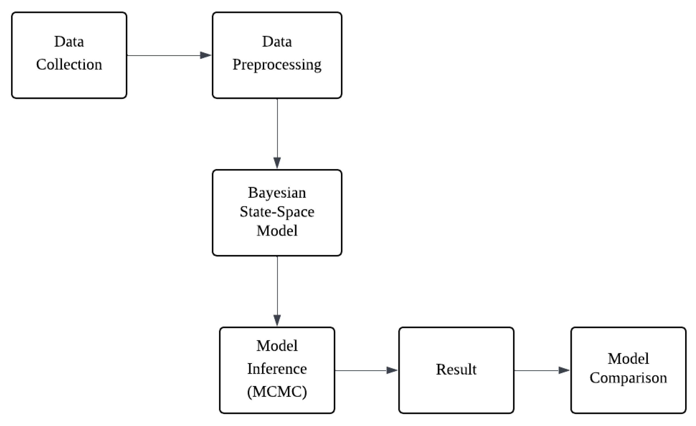
Yahoo Finance (yfinance API) was used for the dataset, and then the preprocessing techniques helped to clean, transform and structure it to make it more suitable and interpretable for the model. It also includes handling missing values, normalizing, encoding categorical variables and ensuring that the data will be well formatted for optimal model performance. After the preprocessing, Bayesian State-Space Model with Autoregressive (AR1) was implemented to predict the stock price for the next 15 days. To estimate the posterior distribution, Markov Chain Monte Carlo (MCMC) was employed by using No-U-Turn sampler (NUTS) to ensure proper convergence of priors. After all the steps, the performance of both models was compared using Mean Square Error (MSE) and Mean Absolute Error (MAE) to determine the predictive accuracy. The flowchart of the workflow is provided for better understanding [32].
Figure 2 illustrates the Bayesian modeling pipeline, starting from data collection and preprocessing, followed by state-space model construction, MCMC-based inference and concluding with the results and model comparison.

3.4. Model Formulation of Bayesian State-Space Model

Bayesian State-Space model:
x t = 0.8 · x t 1 + β X t 1 + s t mod 4 + ϵ t
x t N 0.8 · x t 1 + β X t 1 + Seasonality , σ process 2
where
  • x t is the latent state at time t, representing the underlying Bitcoin price process.
  • x t 1 is the previous latent state.
  • X t 1 is the feature vector at time t 1 .
  • β represents the feature coefficients.
  • Seasonality accounts for periodic fluctuations in price patterns.
  • σ process is the latent state noise, drawn from a half-normal prior distribution to enforce non-negativity.
y t StudentT ν = 4 , μ = x t , σ = σ noise
where
  • y t is the observed Bitcoin closing price at time t.
  • x t is the latent state obtained from the transition model.
  • σ noise is the observation noise, modeled using half-normal prior to control variance.
  • A Student’s t-distribution with 4 degrees of freedom is chosen instead of a Gaussian likelihood to ensure robustness against extreme price fluctuations (outliers).
Here, the use of Student’s t-distribution with ν = 4 is motivated by the heavy-tailed nature of cryptocurrency price changes, which often exhibit large jumps and drops. This specification mitigates the influence of extreme outliers, which occur more frequently than under a Gaussian model. A Gaussian likelihood would produce narrower prediction intervals but is more sensitive to these extreme values. On the other hand, very heavy-tailed choices ( ν < 3 ) would be more robust to outliers but at the cost of overly wide intervals, reducing their usefulness for decision-making.
  • Bayesian State-Space Model (AR1) Sampling Process MCMC with NUTS
For the state-space model, the latent states x t evolve over time with an autoregressive structure and exogenous features [33,34]. The main challenge in sampling arises due to the dependency between successive latent states [35]. On the other hand, the No-U-Turn Sampler (NUTS) was used to make the exploration more efficient in the high-dimensional parameter space by automatically tuning the step sizes and trajectory lengths [36]. The sampling process is outlined below:
  • Define the Posterior Distribution
The posterior is proportional to the product of the likelihood function [37] and the prior distribution:
p ( x , θ y ) p ( y x , θ ) p ( x θ ) p ( θ )
where
  • x are the latent states.
  • θ includes process noise, observation noise, regression coefficients and seasonal components.
  • Hamiltonian Monte Carlo Framework
Introduce an auxiliary momentum variable r N ( 0 , M ) to simulate a Hamiltonian system:
H ( x , r ) = U ( x ) + K ( r )
where
  • Potential Energy: U ( x ) = log p ( x y ) , derived from the posterior distribution.
  • Kinetic Energy: K ( r ) = 1 2 r M 1 r , based on the auxiliary momentum variable r.
  • Leapfrog Integration
Iteratively update the momentum r and latent state x using the leapfrog method.
r t + 1 2 = r t ϵ 2 U ( x t ) x t + 1 = x t + ϵ M 1 r t + 1 2 r t + 1 = r t + 1 2 ϵ 2 U ( x t + 1 )
The step size ϵ and mass matrix M are dynamically adjusted for efficiency.
  • Acceptance Step (Metropolis–Hastings Criterion)
  • A new sample x * is accepted with probability:
    α = min 1 , p ( y x * ) p ( x * ) p ( y x ) p ( x )
  • If u < α (where u U ( 0 , 1 ) ), accept x * ; otherwise, retain x.

3.5. LSTM Neural Network Model

The LSTM model was implemented as deep sequential architecture, which was designed to capture the temporal patterns of Bitcoin price movements. It consisted of four layers, with 60 units in the first and 120 units in the remaining layers and each were followed by dropout to reduce overfitting. A 60-day lookback window of Min–Max normalized features was used as input and the model was trained with the Adam optimizer using MSE as the loss and MAE as an additional evaluation metric. Hyperparameters such as layer sizes and dropout rates were determined empirically through experimentation and this configuration consistently produced the lowest validation errors. The increasing number of units across layers allowed the network to capture progressively more complex dependencies, while dropout ensured generalization without sacrificing the learning capacity [38,39].
  • Model Formulation of LSTM Neural Network
Let the input sequence be:
X = { x 1 , x 2 , , x T } , x t R d
where T is the time window length and d is the number of input features.
  • LSTM Layer Computation
Each LSTM unit at time step t updates its gates, cell state, and hidden state as follows:
f t = σ ( W f [ h t 1 , x t ] + b f ) ( forget gate ) i t = σ ( W i [ h t 1 , x t ] + b i ) ( input gate ) c ˜ t = tanh ( W c [ h t 1 , x t ] + b c ) ( candidate state ) c t = f t c t 1 + i t c ˜ t ( cell state update ) o t = σ ( W o [ h t 1 , x t ] + b o ) ( output gate ) h t = o t tanh ( c t ) ( hidden state )
where
  • f t , i t , o t R u are the forget, input, and output gates,
  • c t , h t R u are the cell and hidden states,
  • u is the number of LSTM units,
  • σ ( · ) is the sigmoid activation function,
  • ⊙ denotes elementwise multiplication.
  • Dropout Regularization
After each LSTM layer, a dropout mask D ( p ) with probability p is applied to the hidden states:
h ^ t = D ( p ) ( h t ) ,
where p = { 0.2 , 0.3 , 0.4 , 0.5 } across the four stacked LSTM layers.
  • Stacked LSTM Layers
The network consists of four LSTM layers with hidden sizes
u = { 60 , 120 , 120 , 120 } .
Stacking enables learning hierarchical temporal representations, where earlier layers capture short-term dependencies and deeper layers capture long-term structures.
  • Output Layer
The final hidden representation is mapped to the output through a fully connected layer:
y ^ t = W d h t + b d ,
where y ^ t R represents the predicted Bitcoin closing price.
  • Loss Function
The model is trained using Mean Squared Error (MSE):
L MSE = 1 N i = 1 N ( y i y ^ i ) 2 ,
with Mean Absolute Error (MAE) monitored as an additional evaluation metric.
  • LSTM Memory Cell Architecture
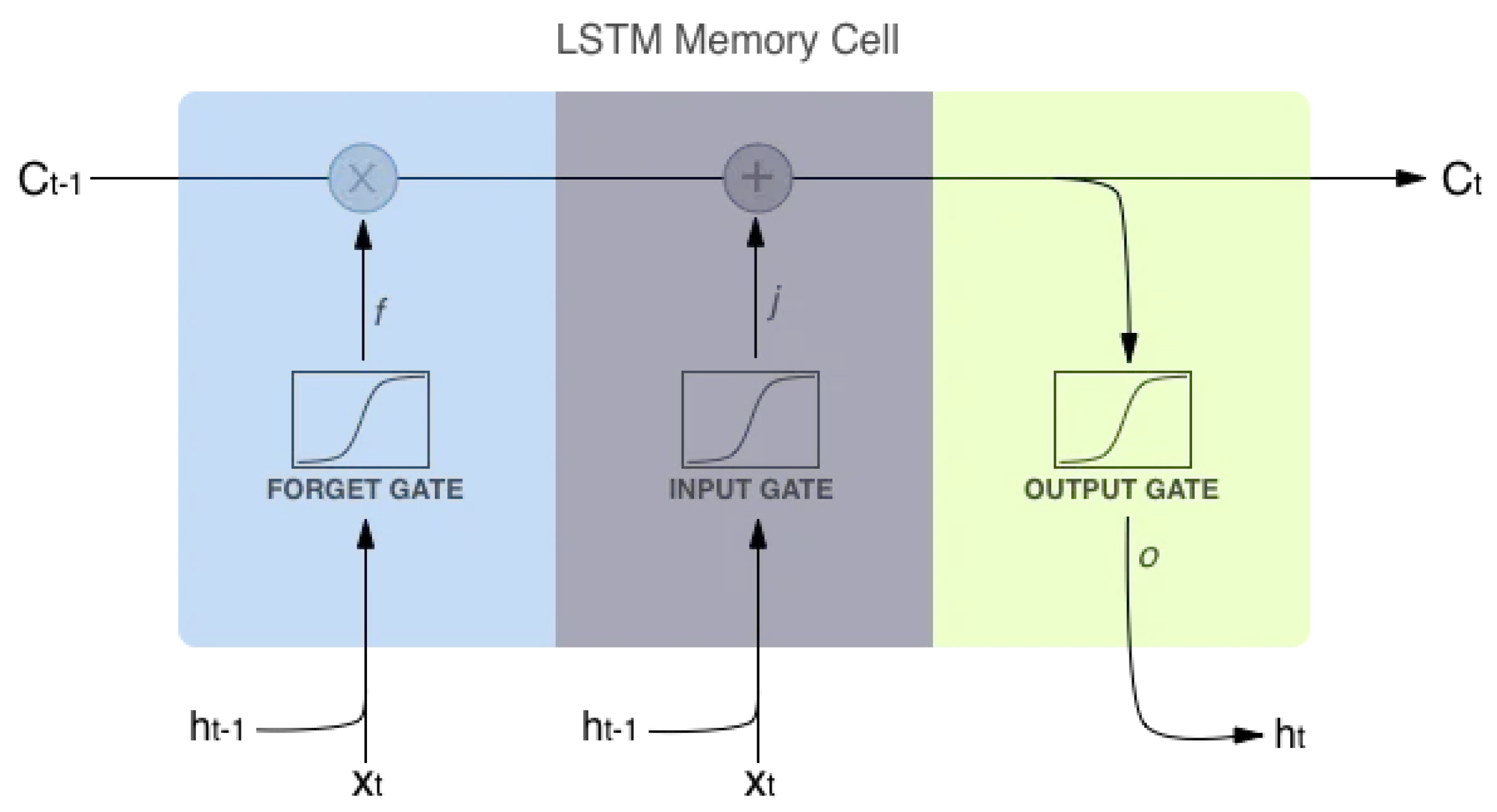
Figure 3 shows the structure of an LSTM memory cell, where the forget, input and output gates regulate information flow by enabling the model to retain long-term dependencies while updating hidden states. In the figure, the LSTM memory cell diagram shows how information flows through three gating mechanisms to produce updated internal states. At each time step t, the input vector x t and the previous hidden state h t 1 are fed into the network. The forget gate f is controlling how much of the previous cell state C t 1 should be retained. The input gate in here j (commonly denoted as i t in equations) determines how much new information should be added to the cell. The resulting cell state C t is being updated by combining the retained memory and new candidate input. The output gate o is regulating how much of the updated cell state should be exposed as the new hidden state h t , which is also the output of the LSTM unit. This gating structure allows the network to not only control information flow but also to maintain long-term dependencies [40,41].
Table 3 summarizes the architecture of the LSTM model, consisting of four stacked LSTM layers with dropout for regularization and a final dense layer for output. The network has a total of 335,161 trainable parameters, which enables it to capture both short- and long-term dependencies in the data.

3.6. Evaluation Metrics

The performance of the forecasting models was evaluated by the two widely used regression metrics named Mean Squared Error (MSE) and Mean Absolute Error (MAE) [42,43]. MSE calculates the average of the squared differences between predicted and actual values by giving a higher weight to the larger errors and makes it suitable for identifying models that produce consistently accurate forecasts. On the other hand, MAE can calculate the average absolute difference between the predicted and actual values and offers a more interpretable error metric comparatively less sensitive to outliers. Both of the metrics were computed separately for training and testing datasets to assess model accuracy and generalization capability. The evaluation approach was applied for both the Bayesian and LSTM models for comparative analysis. The scores are shown in the table.

4. Results

In this section, the results of the Bitcoin price prediction experiments using two distinct approaches, named the Bayesian State-Space model and Long Short-Term Memory (LSTM) neural networks, are presented. The models were evaluated by standard performance metrics, including Mean Squared error (MSE), Mean Absolute Error (MAE), Root Mean Squared Error (RMSE) and the coefficient of determination (R2).
Figure 4 shows the daily closing price of Bitcoin from January 2024 to May 2025. It constitutes the full data window used in this study for forecasting purposes. This period captures a variety of market conditions including gradual uptrends, abrupt price surges, volatility clusters and downward corrections. It ensures the inclusion of both stable and turbulent phases by allowing the forecasting models to learn from a diverse set of temporal patterns and data. Here, the raw closing prices were log-transformed to stabilize variance by reducing large fluctuations and making the series more stationary, which enables the model to better capture underlying patterns and trends.

4.1. Results of Bayesian State-Space Modeling for Cryptocurrency Forecasting

The Bayesian Structural Time Series (BSTS) model was used to forecast the cryptocurrency prices. The model includes an AR(1) component. It helps analyze past price movements and predict future trends. The model was trained using the historical data and tested with new data to analyze the performance. The results of the graph are shown below.
Figure 5 illustrates the performance of the Bayesian State-Space model on the training dataset by showing close alignment between predicted and actual Bitcoin prices, which indicates a strong fit during training.

4.2. Model Evaluation for Bayesian State-Space Model

Here, in Figure 2, it can be seen that the model closely tracks actual price movement in the training dataset. The predicted values match well with the actual values. Therefore, the model can capture the market trends effectively. The 95% credible interval (CI) is narrow during training. This means there is low uncertainty in the predictions.
Figure 6 presents the Bayesian State-Space model’s predictions against actual Bitcoin prices on the test dataset, which highlights its ability to capture overall trends while revealing differences in generalization compared to training performance.
Table 4 reports the estimated coefficients of the Bayesian State-Space model along with their posterior uncertainty. The table presents the mean, median and 95% credible intervals for each beta coefficient, showing both significant effects (e.g., Beta 1) and parameters with wide intervals indicating higher uncertainty.
Process Standard Deviation
MeanMedianLower CI (2.5%)Upper CI (97.5%)
0.0254520.0254540.0224580.028671
Noise Standard Deviation
MeanMedianLower CI (2.5%)Upper CI (97.5%)
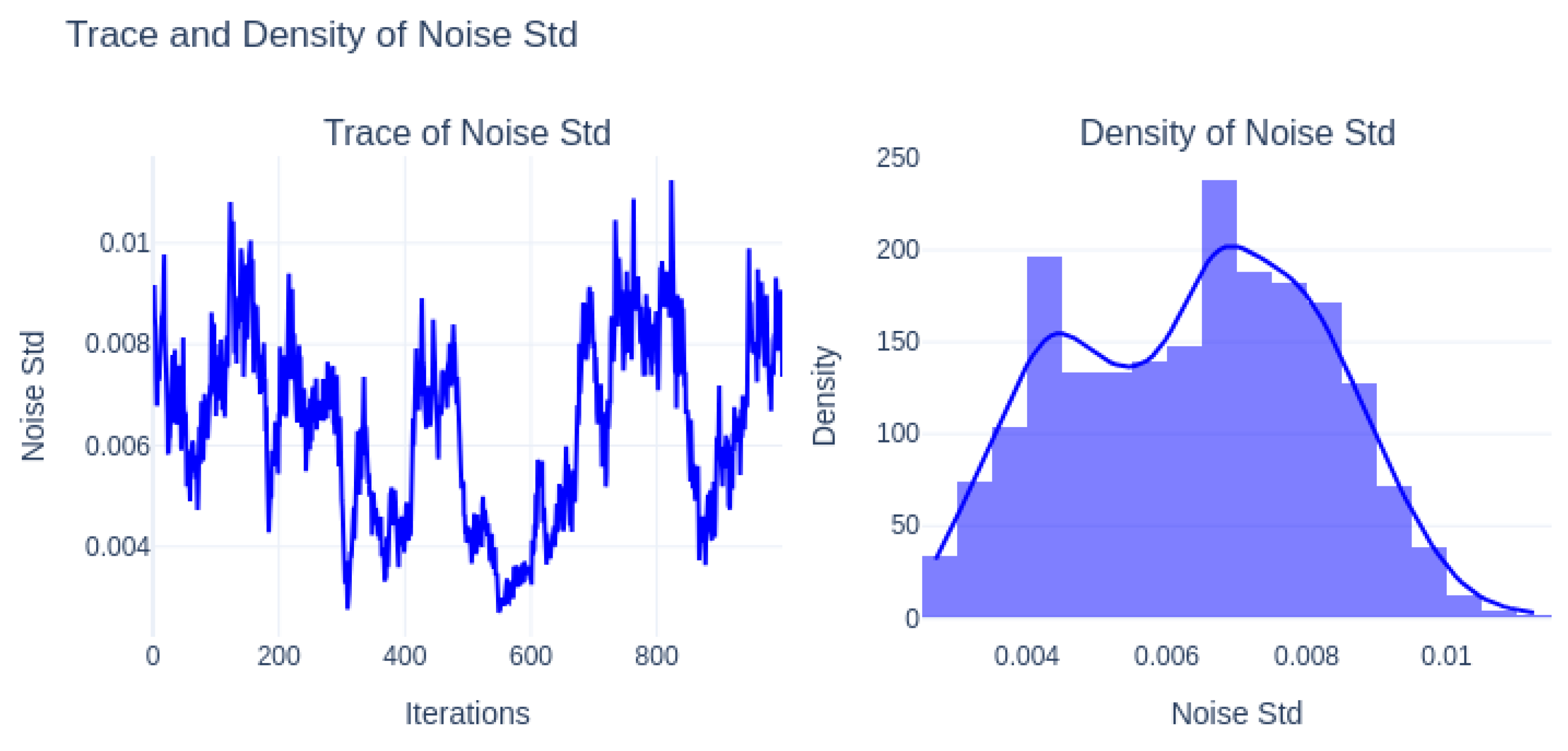
0.0063690.0065840.0031470.009534
Process Standard Deviation: Here, Mean: 0.02545 is pointing to moderate variability over time in the latent state transitions.
Noise Standard Deviation: On the other hand, the noise standard deviation of Mean: 0.00637 is reflecting low observation-level noise and suggesting high fidelity between latent states with observed data.
Figure 7 displays the convergence diagnostics for the Bayesian State-Space model’s beta coefficients, showing stable trace plots that indicate good mixing and reliable posterior sampling.
Convergence Diagnostics of Beta Coefficients: The trace plot displays the MCMC sampling for the nine β coefficients over 1000 iterations. All the chains show good mixing and fluctuations around stable mean values with no signs of divergence or drift in it. Therefore, the Markov chains have converged properly and the posterior samples for the coefficients are reliable for the inference.
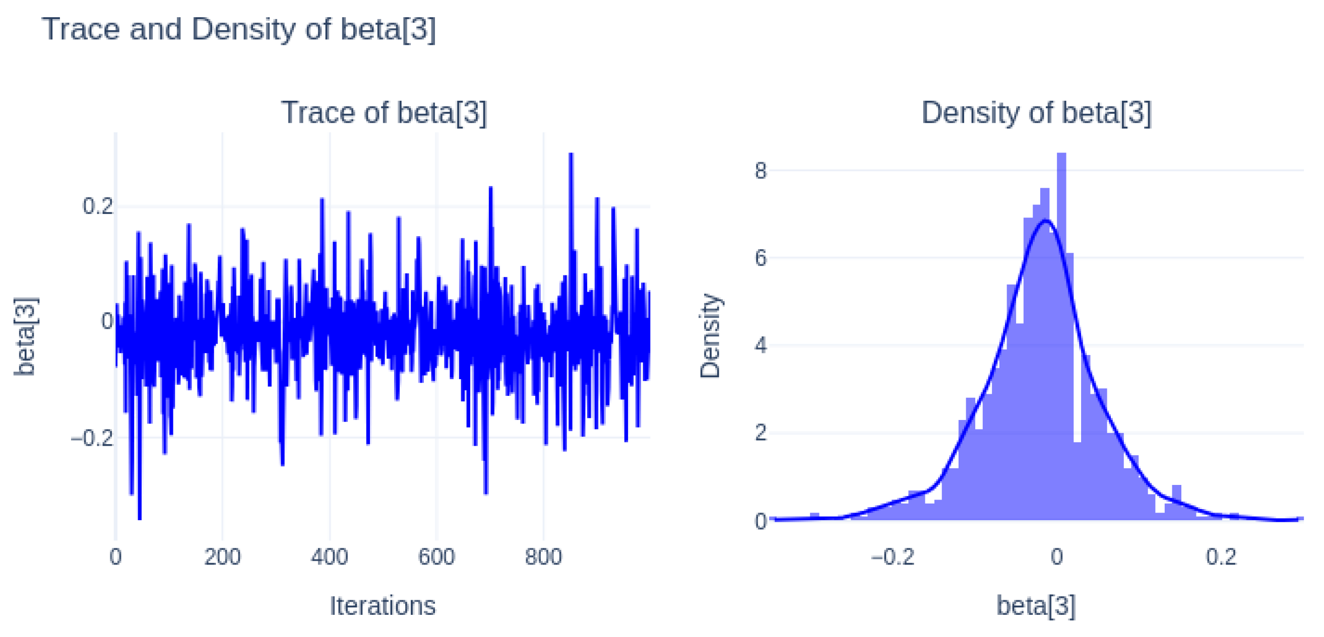
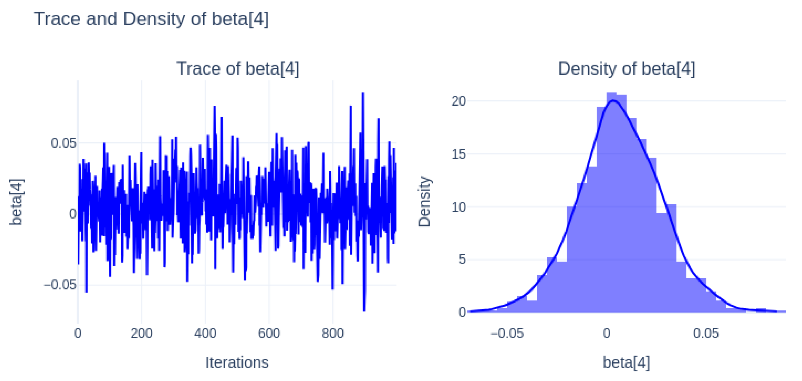
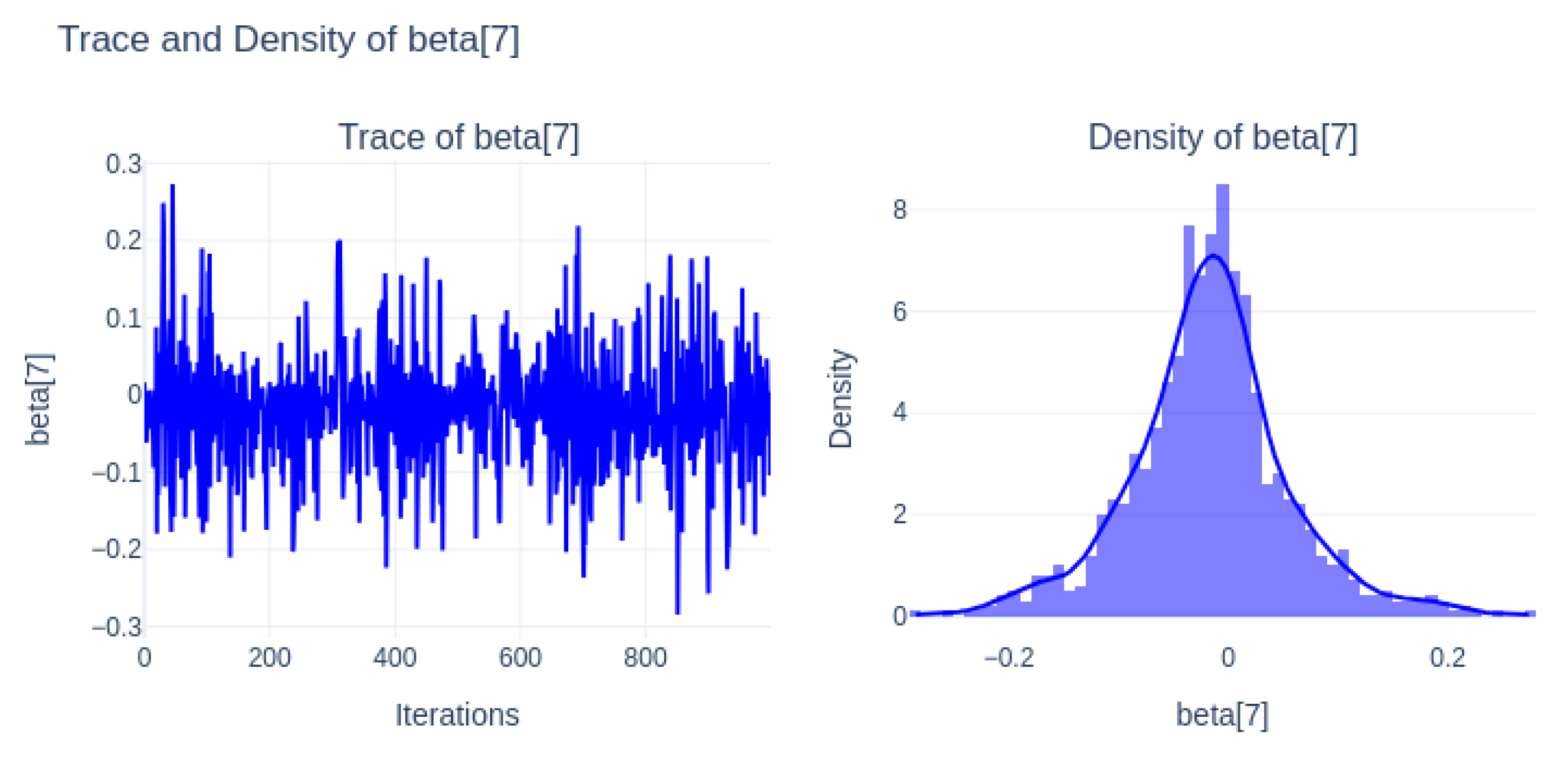
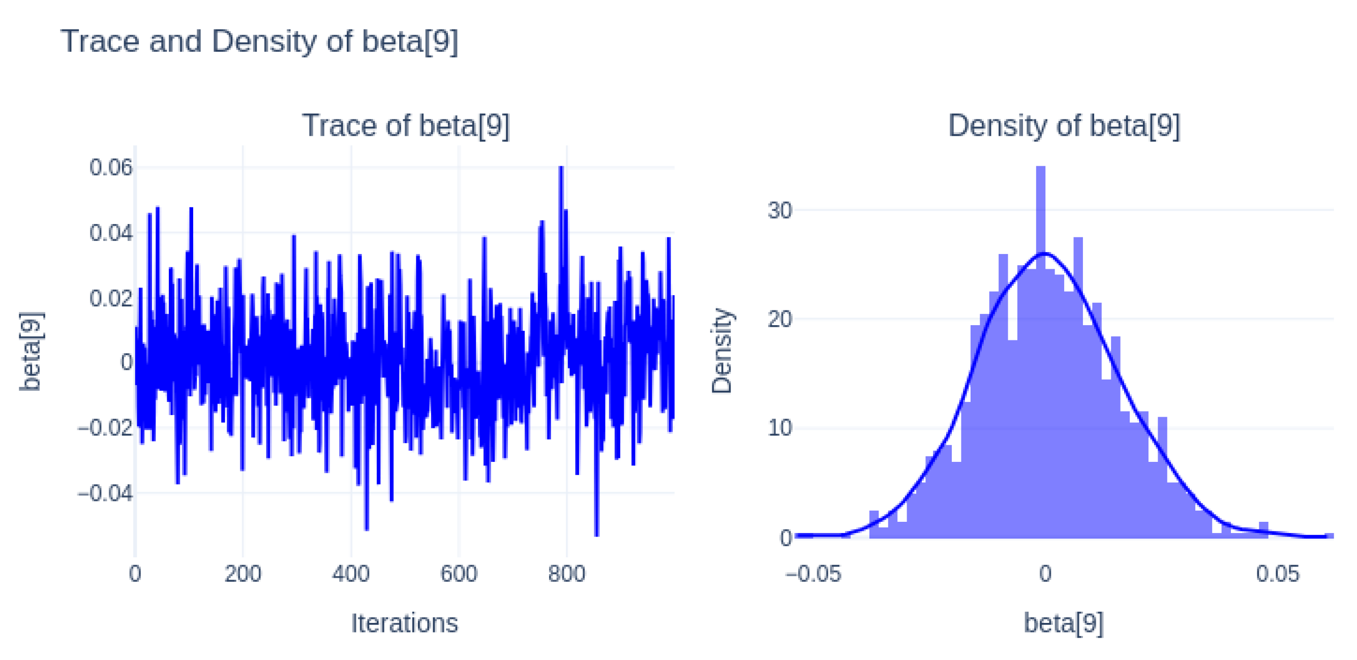
Trace and Density of Process Standard Deviation: The trace plots for all nine β coefficients shows well-mixed and stationary sampling behavior and fluctuations without visible drifts or autocorrection around the consistent mean values across iterations. It indicates a good convergence and reliable sampling from the posterior distribution. On the other hand, the corresponding density plots for each β . It reveals approximately symmetric and unimodal distributions among which many of them resemble the Gaussian shapes. However, the distributions vary in spread and central tendency by reflecting the individual influence and uncertainty of each predictor in the state-space model. On the contrary, some coefficients like β 3 and β 7 showed wider credible intervals by indicating higher uncertainty, while others are more tightly concentrated with more stable posterior estimates.
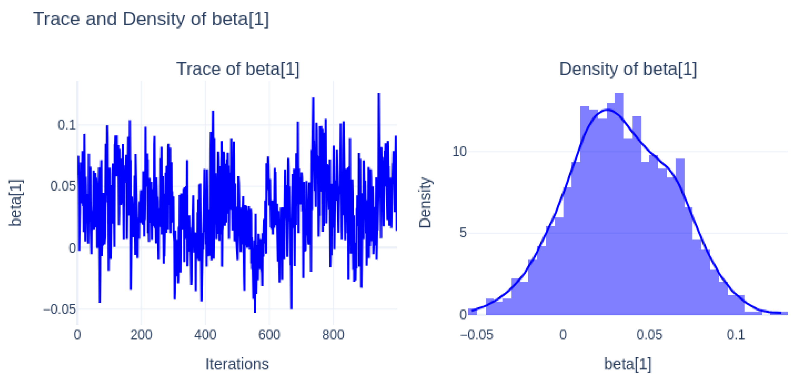
Figure 8 (beta[1]) shows stable trace plots with good mixing and a well-centered density distribution, indicating reliable posterior estimates.
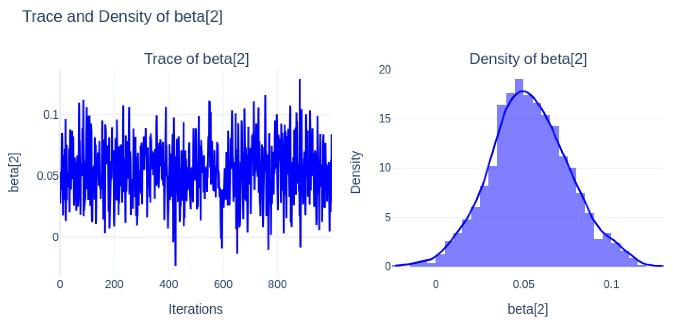
Figure 9 (beta[2]) demonstrates clear convergence, and its density indicates a significant positive effect with narrow credible intervals.
Figure 10 (beta[3]) shows wider posterior uncertainty with a centered distribution close to zero, suggesting limited explanatory power.
Figure 11 (beta[4]) has well-mixed chains and a density concentrated around small values, indicating minor influence on the model.
Figure 12 (beta[5]) also shows narrow density around near-zero, with stable convergence, reflecting a weak contribution.
Figure 13 (beta[6]) presents higher posterior variability and wider density, suggesting uncertainty in its role within the model.
Figure 14 (beta[7]) converges properly but remains centered near zero, indicating negligible effect.
Figure 15 (beta[8]) has a flat, wider posterior distribution around zero, highlighting uncertainty and low importance.
Figure 16 (beta[9]) shows well-mixed chains and a posterior centered close to zero, reflecting minimal influence.
Stationarity and Convergence: The trace plot of the process standard deviation shows the stable oscillations around the mean with no visible trends or divergence, which also indicates that the MCMC chain has converged and is well-mixed. in addition, the corresponding density plot is approximately bell-shaped and symmetric. From the suggestion of the posterior distribution of the process standard deviation, it is unimodal and concentrated. It reflects stable dynamics in the latent state evolution with moderate uncertainty. The trace plots for all β parameters show a stable fluctuation around a central value, indicating the Markov Chain Monte Carlo(MCMC) process has likely reached the convergence. Also, no strong trends or drifts are visible, which is a good indication of stationarity.
Distribution of Parameters and Significance: The posterior distribution of the process standard deviation is unimodal and approximately symmetric, centered around 0.025 with a trace plot that is showing stable mixing and convergence. It also indicates consistent and moderate uncertainty in the evolution of the latent state over time. Furthermore, the noise standard deviation shows a slightly multimodal posterior distribution, where it is indicating more complex or variable measurement noise behavior. Its trace plot shows slower mixing and periodic shifts, which may reflect more heterogeneity or temporal fluctuations in the observation noise. Despite all these, the distributions remain concentrated and bounded by supporting the model’s capacity to represent both latent dynamics and observational uncertainty effectively.
Figure 17 shows the trace and density of the process standard deviation, indicating stable convergence and a well-defined posterior distribution.
Figure 18 presents the trace and density of the noise standard deviation, which also demonstrates proper mixing and a concentrated posterior, suggesting reliable parameter estimation.

4.3. Results of LSTM for Cryptocurrency Forecasting

The Long Short-Term Memory (LSTM) model was used to forecast the logarithmic closing prices of Bitcoin. The architecture consisted of four LSTM layers with progressively increasing dropout rates for preventing overfitting. The model was trained on scaled features and evaluated by using standard performance metrics. On the training data, the model achieved a Mean Squared Error (MSE) of 0.0004, Mean Absolute Error (MAE) of 0.0160, Root Mean Squared Error (RMSE) of 0.0212 and a coefficient of determination ( R 2 ) of 0.9924. The predicted numbers indicate excellent fit. However, the test results showed a noticeable decline in generalization with an MSE of 0.0007, MAE of 0.0212, RMSE of 0.0259 and R 2 of 0.3505. This performance gap is showing the potential overfitting by implying that the model captured noise or short-term fluctuations in the training data, which did not transfer well to unseen samples.
The visualization is demonstrating a strong level of alignment between certain price-related variables and technical indicators, particularly during major upward and downward market shifts. For example, the moving averages and return-based features closely track the overall shape of the price trajectory, suggesting their relevance in capturing trend and momentum signals. Gap-based indicators reflect short-term volatility and abrupt market changes, so it is critical in cryptocurrency forecasting tasks. The figure confirms that external indicators not only co-move with price series but also potentially lead or lag certain market behaviors. These observations justify the inclusion as input features in both deep learning and probabilistic forecasting models.
Figure 19 presents the training loss curves of the LSTM model using Mean Squared Error (MSE) and Mean Absolute Error (MAE). The steady decline and stabilization of both metrics across epochs indicate effective learning and absence of severe overfitting.
Here, the figure shows the training loss of the LSTM model across 250 epochs by evaluating using two metrics: Mean Squared Error (MSE) and Mean Absolute Error (MAE). Both loss functions showed a steep decline during the early training phase—particularly within the first 20 epochs by indicating rapid convergence as the model begins to learn the underlying structure of the Bitcoin time series data. Beyond this point, the curves flatten and show minimal fluctuation, suggesting that the model reaches a stable training state. The consistently lower MSE values compared with the MAE reflects the stronger penalization of large errors, which is beneficial for capturing significant deviations in price movement. The most important point will be the absence of sharp oscillations or divergence in either metric, which will imply that the model is not overfitting and maintains a smooth generalization behavior throughout the training.
Figure 20 illustrates the performance of the LSTM model in forecasting the logarithmic closing prices of Bitcoin. The graph presents both training and testing results by showing actual values against predicted values over the period from early 2024 to mid-2025. The training predictions align closely with the actual values by reflecting a strong learning experience. In the test segment, although the predictions follow the overall trend, a visible divergence is observed in some short-term fluctuations, which indicates reduced generalization capability. This gap between training and testing accuracy highlights the importance of incorporating additional regularization or hybrid approaches to improve robustness in unseen data.

4.4. Summary of Model Performance

In both training and testing phases, the Bayesian State-Space model and the LSTM model demonstrate their strengths. The Bayesian State-Space model achieved the superior performance on the training set with a lower MSE of 0.0000 and MAE of 0.0026, which indicates a strong fit to the training data, and MSE of 0.0013 and MAE of 0.0307 for test data. On the contrary, the LSTM model demonstrated better generalization capability, with MSE of 0.0004 and MAE of 0.0160 for training and MSE of 0.0007 and MAE of 0.0212 for the test dataset. The Bayesian model is more precise in capturing historical patterns, and LSTM is better for adapting to unseen data in dynamic market conditions. Bayesian has lower MSE and MAE, which means that it fits the data more perfectly than LSTM, yet the LSTM model is more precise on unseen data.
Table 5 summarizes the training and testing errors for both models. The Bayesian State-Space model achieved the lowest training error, indicating a strong fit to the training data, but showed higher test errors, suggesting some degree of overfitting. In contrast, the LSTM exhibited slightly higher training error but lower test error, highlighting its better generalization to unseen data.

4.5. Correlating Matrix

Figure 21 shows the heatmap of the correlation matrix between the input features and Log_Close that were used in both LSTM and Bayesian models. From the heatmap, strong correlations are observed among the price-based variables while some features showed more independent behavior. Here, the Pearson correlation coefficient was implemented in the .corr() function of the Pandas library.
Table 6 presents the correlations of all input features with Log_Close, which served as the primary target variable in both LSTM and Bayesian models. As expected, the price-based features such as Close, High, Low, Open and moving averages (SMA_7 and SMA_30) exhibit very strong correlations with Log_Close, confirming their predictive relevance. In contrast, the features such as returns, gaps and categorical encodings (e.g., volume gap lmh, daily change lmh) show weak or even negligible correlations, indicating their complementary rather than direct predictive role.

5. Conclusions

This study compared the performance of the logarithmic closing prices of Bitcoin by using Long Short-Term Memory (LSTM) of neural networks and Bayesian state-space models in forecasting. The models were trained using a wide range of technical indicators and engineered features. The LSTM model achieved a training MAE of 0.0160 and MSE of 0.0004, while on the test set, it achieved an MAE of 0.0212 and MSE of 0.0007. In contrast, the Bayesian model demonstrated a training MAE of 0.0026 and MSE of 0.0000, where the test performance was weaker than LSTM, with an MAE of 0.0307 and MSE of 0.0013.
The results indicate that the Bayesian model fits exceptionally well for the training data but faces difficulties with reduced generalization on unseen data. The LSTM model, on the other hand, offers a better balance between in-sample accuracy and out-of-sample generalization. The strong influence of core market variables were highlighted by the correlation analysis and their lagged counterparts by confirming their importance in forecasting accuracy. In contrast, features with weaker correlations like engineered indicators may contribute complementary non-linear signals that enhance model diversity and depth. Particularly in neural network architectures. Future work may be explored by combining LSTM and Bayesian approaches or integrating external information such as macroeconomic indicators and sentiment data to improve predictive stability and adaptability in the highly volatile cryptocurrency domain.
While the Bayesian State-Space model achieved low training error, the higher test error compared to the LSTM suggests that it may overfit to the training data. The LSTM, on the other hand, had slightly higher training error and produced lower test MSE and MAE, which indicates better generalization, stemming from the model’s output nature. The LSTM provides a single point prediction that aims at minimizing average error, where the Bayesian model outputs both prediction and a credible interval that covers a wider range of possible outcomes to reflect uncertainty. Therefore, the LSTM is preferable when point accuracy is the priority, and the Bayesian approach is advantageous when uncertainty estimation is also important.

Author Contributions

Conceptualization, B.B.B. and M.R.; methodology, software, formal analysis, writing—original draft preparation, B.B.B.; software, M.R.; validation, M.R., M.J.A. and S.S.; data curation, visualization, writing—review and editing, M.R.; supervision, project administration, writing—review and editing, A.T. and M.S.; investigation, funding acquisition, A.T.; writing—review and editing, M.J.A. and S.S.; resources, M.J.A. and S.S.; visualization, B.B.B. and M.R. All authors have read and agreed to the published version of the manuscript.

Funding

This research will be funded by the University of Miyazaki, Japan, following acceptance and publication of the article.

Institutional Review Board Statement

Not applicable.

Informed Consent Statement

Not applicable.

Data Availability Statement

The data used in this study were collected from Yahoo Finance (https://finance.yahoo.com/quote/BTC-USD/) (accessed on 15 April 2025).

Acknowledgments

The authors gratefully acknowledge the University of Miyazaki, Japan, and the Technical University of Dortmund, Germany, for providing computational resources and research support. Special thanks to academic supervisors for their continuous guidance and encouragement.

Conflicts of Interest

The authors declare no conflicts of interest.

References

  1. Vora, G. Cryptocurrencies: Are Disruptive Financial Innovations Here? Mod. Econ. 2015, 6, 816–832. [Google Scholar] [CrossRef]
  2. Almagsoosi, L.; Abadi, M.; Hasan, H.F.; Sharaf, H. Effect of the Volatility of the Crypto Currency and Its Effect on the Market Returns. Ind. Eng. Manag. Syst. 2022, 21, 238–243. [Google Scholar] [CrossRef]
  3. Ahmed, M.S.; El-Masry, A.A.; Al-Maghyereh, A.I.; Kumar, S. Cryptocurrency Volatility: A Review, Synthesis, and Research Agenda. Res. Int. Bus. Financ. 2024, 71, 102472. [Google Scholar] [CrossRef]
  4. Brini, A.; Lenz, J. A Comparison of Cryptocurrency Volatility—Benchmarking New and Mature Asset Classes. Financ. Innov. 2024, 10, 122. [Google Scholar] [CrossRef]
  5. Habib, G.; Sharma, S.; Ibrahim, S.; Ahmad, I.; Qureshi, S.; Ishfaq, M. Blockchain Technology: Benefits, Challenges, Applications, and Integration of Blockchain Technology with Cloud Computing. Future Internet 2022, 14, 341. [Google Scholar] [CrossRef]
  6. Xu, M.; Chen, X.; Kou, G. A Systematic Review of Blockchain. Financ. Innov. 2019, 5, 27. [Google Scholar] [CrossRef]
  7. Panda, S.K.; Sathya, A.R.; Das, S. Bitcoin: Beginning of the Cryptocurrency Era. In Recent Advances in Blockchain Technology: Real-World Applications; Panda, S.K., Sathya, A.R., Das, S., Eds.; Lecture Notes in Networks and Systems; Springer: Cham, Switzerland, 2023; Volume 560, pp. 11–23. [Google Scholar] [CrossRef]
  8. Fatima, S.S.W.; Rahimi, A. A Review of Time-Series Forecasting Algorithms for Industrial Manufacturing Systems. Machines 2024, 12, 380. [Google Scholar] [CrossRef]
  9. Alaminos, D.; Salas, M.B.; Partal-Ureña, A. Hybrid ARMA-GARCH-Neural Networks for Intraday Strategy Exploration in High-Frequency Trading. Pattern Recognit. 2024, 148, 110139. [Google Scholar] [CrossRef]
  10. Seabe, P.L.; Moutsinga, C.R.B.; Pindza, E. Forecasting Cryptocurrency Prices Using LSTM, GRU, and Bi-Directional LSTM: A Deep Learning Approach. Fractal Fract. 2023, 7, 203. [Google Scholar] [CrossRef]
  11. Khedr, A.; Arif, I.; P V, P.; El-Bannany, M.; Alhashmi, M.; Sreedharan, M. Cryptocurrency Price Prediction Using Traditional Statistical and Machine-Learning Techniques: A Survey. Intell. Syst. Account. Financ. Manag. 2021, 28, 3–34. [Google Scholar] [CrossRef]
  12. Beck, J. Bayesian System Identification Based on Probability Logic. Struct. Control Health Monit. 2010, 17, 825–847. [Google Scholar] [CrossRef]
  13. Kaplan, D. On the Quantification of Model Uncertainty: A Bayesian Perspective. Psychometrika 2021, 86, 215–238. [Google Scholar] [CrossRef]
  14. Singh, V.; Sahana, S.K.; Bhattacharjee, V. A Novel CNN-GRU-LSTM Based Deep Learning Model for Accurate Traffic Prediction. Discov. Comput. 2025, 28, 38. [Google Scholar] [CrossRef]
  15. Gupta, P.; Malik, S.; Apoorb, K.; Sameer, S.; Vardhan, V.; Ragam, P. Stock Market Analysis Using Long Short-Term Model. ICST Trans. Scalable Inf. Syst. 2023, 11, 2. [Google Scholar] [CrossRef]
  16. Yahoo Finance. Bitcoin USD (BTC-USD) Stock Price, News, Quote & History. Available online: https://finance.yahoo.com/quote/BTC-USD/ (accessed on 15 April 2025).
  17. Hua, Y.; Zhao, Z.; Li, R.; Chen, X.; Liu, Z.; Zhang, H. Deep Learning with Long Short-Term Memory for Time Series Prediction. IEEE Commun. Mag. 2019, 57, 114–119. [Google Scholar] [CrossRef]
  18. Suleman, M.A.R.; Shridevi, S. Short-Term Weather Forecasting Using Spatial Feature Attention Based LSTM Model. IEEE Access 2022, 10, 82456–82468. [Google Scholar] [CrossRef]
  19. Teye, M.; Azizpour, H.; Smith, K. Bayesian Uncertainty Estimation for Batch Normalized Deep Networks. arXiv 2018, arXiv:1802.06455. [Google Scholar] [CrossRef]
  20. Kervancı, H.; Akay, D.; Özceylan, E. Bitcoin price prediction using LSTM, GRU and hybrid LSTM-GRU with Bayesian optimization, random search, and grid search for the next days. J. Ind. Manag. Optim. 2023, 20, 570–588. [Google Scholar] [CrossRef]
  21. Ante, L. How Elon Musk’s Twitter activity moves cryptocurrency markets. Financ. Res. Lett. 2021, 38, 101539. [Google Scholar] [CrossRef]
  22. Pandey, T.D. Impact of Musk’s Remarks on Volatility of Bitcoin and Dogecoin Amid COVID-19 Pandemic. J. Digit. Econ. 2024, 3, 85–102. [Google Scholar] [CrossRef]
  23. Huynh, T.L.D. When Elon Musk Changes His Tone, Does Bitcoin Adjust Its Tune? Comput. Econ. 2023, 62, 639–661. [Google Scholar] [CrossRef]
  24. Seabe, P.L.; Moutsinga, C.R.B.; Pindza, E. Sentiment-Driven Cryptocurrency Forecasting: Analyzing LSTM, GRU, Bi-LSTM, and Temporal Attention Model (TAM). Soc. Netw. Anal. Min. 2025, 15, 52. [Google Scholar] [CrossRef]
  25. Kavitha, K.; Gopi, K.; Saicharan, K.; Tharun, K.; Abhinay, K. Cryptocurrency Price Forecasting with Sentiment-Driven Alerts Using ML. Int. J. Innov. Res. Sci. Eng. Technol. 2025, 14, 9280–9287. [Google Scholar]
  26. Kabo, I.G.; Obunadike, G.N.; Samaila, N.A. Sentiment-Driven and Economic Indicators for Bitcoin Price Forecasting: A Hybrid Time Series Model. J. Sci. Res. Rev. 2025, 2, 99–107. [Google Scholar] [CrossRef]
  27. Wen, C.; Wu, X.; Shen, C.; Huang, Z.; Cai, P. Bitcoin Price Prediction Based on Sentiment Analysis and LSTM. Appl. Comput. Eng. 2023, 29, 148–159. [Google Scholar] [CrossRef]
  28. Hamayel, M.J.; Owda, A.Y. A Novel Cryptocurrency Price Prediction Model Using GRU, LSTM and bi-LSTM Machine Learning Algorithms. AI 2021, 2, 477–496. [Google Scholar] [CrossRef]
  29. Tripathi, B.; Sharma, R.K. Modeling Bitcoin Prices Using Signal Processing Methods, Bayesian Optimization, and Deep Neural Networks. Comput. Econ. 2023, 62, 1919–1945. [Google Scholar] [CrossRef]
  30. Ghosh, P.M. Customer Conversion Prediction with Markov Chain Classifier. 2015. Available online: https://pkghosh.wordpress.com/2015/07/06/customer-conversion-prediction-with-markov-chain-classifier/ (accessed on 17 August 2025).
  31. Amunategui, M. Markov Chains—Seeing the Future. 2015. Available online: https://amunategui.github.io/markov-chains/index.html (accessed on 17 August 2025).
  32. Muhammad, M.; Abba, B. A Bayesian Inference with Hamiltonian Monte Carlo (HMC) Framework for a Three-Parameter Model with Reliability Applications. Kuwait J. Sci. 2025, 52, 100365. [Google Scholar] [CrossRef]
  33. Noomene, R. Procedures of Parameters’ Estimation of AR(1) Models into Linear State-Space Models. In Proceedings of the World Congress on Engineering 2007 (WCE 2007), London, UK, 2–4 July 2007; Volume II; Lecture Notes in Engineering and Computer Science. Newswood Limited: Hong Kong, China, 2007. [Google Scholar]
  34. Cao, Y.; Tufto, J. Bayesian Inference with tmbstan for a State-Space Model with VAR(1) State Equation. arXiv 2021, arXiv:2101.05635. [Google Scholar] [CrossRef]
  35. Zhang, T.; Zhao, S.; Luan, X.; Liu, F. Bayesian Inference for State-Space Models With Student-t Mixture Distributions. IEEE Trans. Cybern. 2023, 53, 4435–4445. [Google Scholar] [CrossRef]
  36. Yuan, K.; Girolami, M.; Niranjan, M. Markov Chain Monte Carlo Methods for State-Space Models with Point Process Observations. Neural Comput. 2012, 24, 1462–1486. [Google Scholar] [CrossRef] [PubMed]
  37. Bernardo, J. Reference Posterior Distributions for Bayesian Inference. J. R. Stat. Soc. Ser. B (Methodol.) 1979, 41, 113–147. [Google Scholar] [CrossRef]
  38. Ghislieri, M.; Cerone, G.L.; Knaflitz, M.; Agostini, V. Long Short-Term Memory (LSTM) Recurrent Neural Network for Muscle Activity Detection. J. Neuroeng. Rehabil. 2021, 18, 153. [Google Scholar] [CrossRef]
  39. Van Houdt, G.; Mosquera, C.; Nápoles, G. A Review on the Long Short-Term Memory Model. Artif. Intell. Rev. 2020, 53, 5929–5955. [Google Scholar] [CrossRef]
  40. ElMoaqet, H.; Eid, M.; Glos, M.; Ryalat, M.; Penzel, T. Deep Recurrent Neural Networks for Automatic Detection of Sleep Apnea from Single Channel Respiration Signals. Sensors 2020, 20, 5037. [Google Scholar] [CrossRef]
  41. Yadav, H.; Thakkar, A. NOA-LSTM: An Efficient LSTM Cell Architecture for Time Series Forecasting. Expert Syst. Appl. 2024, 238, 122333. [Google Scholar] [CrossRef]
  42. Chai, T.; Draxler, R. Root Mean Square Error (RMSE) or Mean Absolute Error (MAE)? Arguments Against Avoiding RMSE in the Literature. Geosci. Model Dev. 2014, 7, 1247–1250. [Google Scholar] [CrossRef]
  43. Hodson, T. Root-Mean-Square Error (RMSE) or Mean Absolute Error (MAE): When to Use Them or Not. Geosci. Model Dev. 2022, 15, 5481–5487. [Google Scholar] [CrossRef]
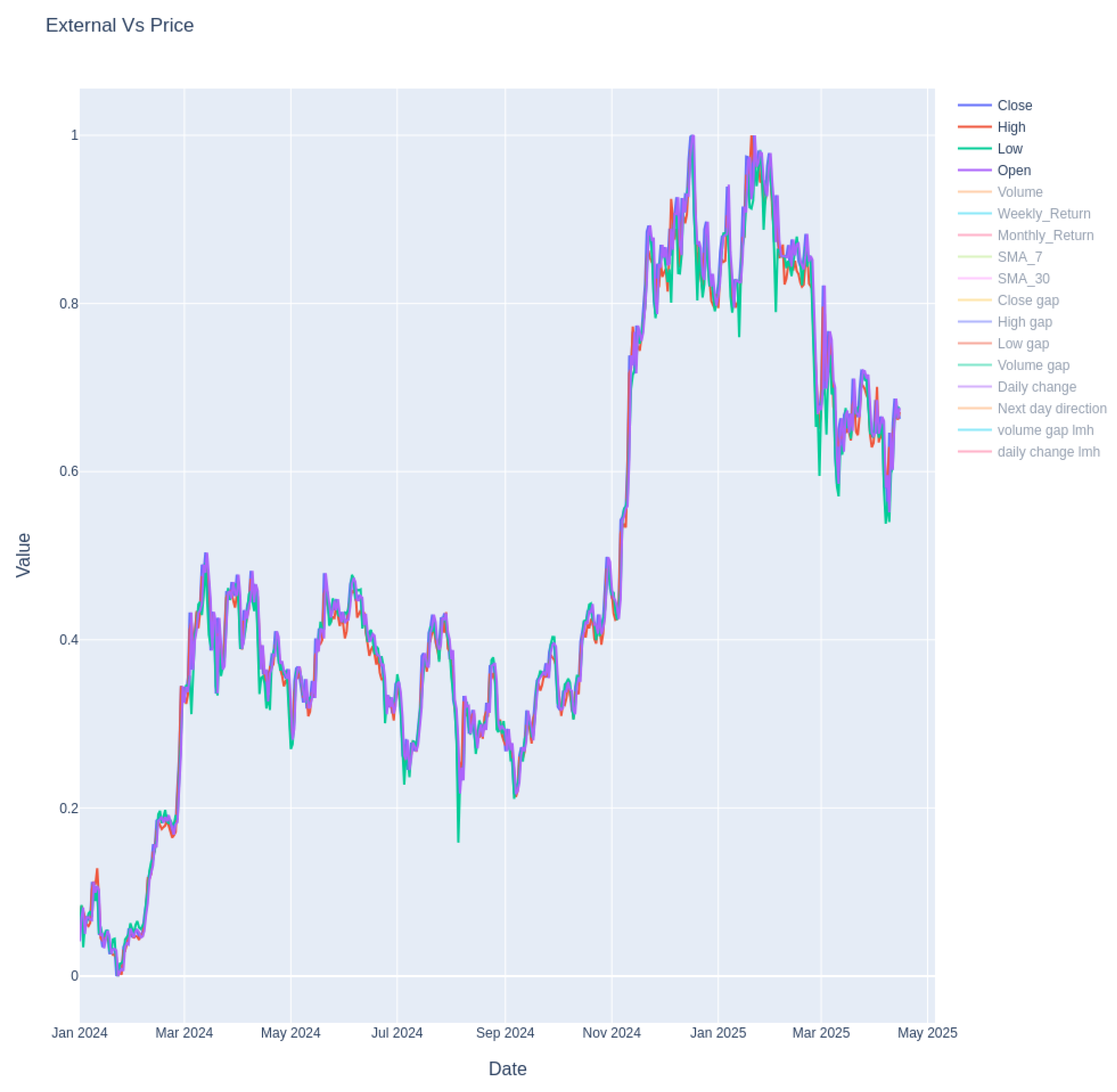
Figure 1. Bitcoin price series and external market indicators.
Informatics 12 00087 g001
Figure 2. Flowchart of the Bayesian modeling pipeline.
Informatics 12 00087 g002
Figure 3. Structure of the LSTM memory cell.
Informatics 12 00087 g003
Figure 4. Considered period for Bitcoin closing price prediction.
Informatics 12 00087 g004
Figure 5. State- Space training predictions vs. actual values.
Informatics 12 00087 g005
Figure 6. State- Space test predictions vs. actual values.
Informatics 12 00087 g006
Figure 7. Convergence diagnostics of beta coefficients.
Informatics 12 00087 g007
Figure 8. Trace and density of beta[1].
Informatics 12 00087 g008
Figure 9. Trace and density of beta[2].
Informatics 12 00087 g009
Figure 10. Trace and density of beta[3].
Informatics 12 00087 g010
Figure 11. Trace and density of beta[4].
Informatics 12 00087 g011
Figure 12. Trace and density of beta[5].
Informatics 12 00087 g012
Figure 13. Trace and Density of beta[6].
Informatics 12 00087 g013
Figure 14. Trace and density of beta[7].
Informatics 12 00087 g014
Figure 15. Trace and density of beta[8].
Informatics 12 00087 g015
Figure 16. Trace and density of beta[9].
Informatics 12 00087 g016
Figure 17. Trace and density of process standard deviation.
Informatics 12 00087 g017
Figure 18. Trace and density of noise standard deviation.
Informatics 12 00087 g018
Figure 19. LSTM training loss curves for MSE and MAE across epochs.
Informatics 12 00087 g019
Figure 20. Actual vs. predicted Log_Close prices using the LSTM model (train and test sets).
Informatics 12 00087 g020
Figure 21. Correlating matrix.
Informatics 12 00087 g021
Table 1. Summary of dataset features and completeness.
ColumnNon-Null CountData Type
Close836float64
High836float64
Low836float64
Open836float64
Volume836int64
Weekly_Return829float64
Monthly_Return806float64
SMA_7830float64
SMA_30807float64
Table 2. Input attributes used in the model.
AttributesTypeDescription
CloseContinuousClosing price of the asset for the trading day.
HighContinuousHighest price of the asset during the trading day.
LowContinuousLowest price of the asset during the trading day.
OpenContinuousThe opening price of the asset at the start of the trading day.
VolumeContinuousTotal number of shares/units traded during the day.
Weekly_ReturnContinuousPercentage return of the asset over the past week.
Monthly_ReturnContinuousPercentage return of the asset over the past month.
SMA_7Continuous7-day Simple Moving Average of the closing price.
SMA_30Continuous30-day Simple Moving Average of the closing price.
Close gapContinuousThe gap between the current day’s close and the previous day’s close.
High gapContinuousThe gap between the current day’s high and the previous day’s high.
Low gapContinuousThe gap between the current day’s low and the previous day’s low.
Volume gapContinuousGap between the current day’s trading volume and the previous day’s volume.
Daily changeContinuousAbsolute or percentage change in price from open to close.
Next day directionCategoricalBinary indicator (0/1) for whether the next day’s price increased or decreased.
Volume gap lmhCategoricalCategorized volume gap as low (L), medium (M), or high (H).
Daily change lmhCategoricalCategorized daily change as low (L), medium (M), or high (H).
Table 3. LSTM sequential model summary.
Layer (Type)Output ShapeParam #
LSTM (lstm)(None, 1, 60)16,800
Dropout (dropout)(None, 1, 60)0
LSTM (lstm_1)(None, 1, 120)86,880
Dropout (dropout_1)(None, 1, 120)0
LSTM (lstm_2)(None, 1, 120)115,680
Dropout (dropout_2)(None, 1, 120)0
LSTM (lstm_3)(None, 120)115,680
Dropout (dropout_3)(None, 120)0
Dense (dense)(None, 1)121
Total params:335,161 (1.28 MB)
Trainable params:335,161 (1.28 MB)
Non-trainable params:0 (0.00 B)
Table 4. Table of Bayesian State-Space model coefficients and uncertainty.
Beta CoefficientMeanMedianLower CI (2.5%)Upper CI (97.5%)
00.0332500.031372−0.0259990.090184
10.0533560.0521670.0095080.100368
2−0.020745−0.018536−0.1799730.135351
30.0065510.006268−0.0346400.048365
40.0040110.003931−0.0012950.009155
50.0021780.001892−0.0086420.014365
6−0.017455−0.016412−0.1750800.144590
7−0.013722−0.012798−0.0451340.015407
80.000599−0.000107−0.0282920.031358
Table 5. Summary of MSE and MAE for Bayesian State-Space model and LSTM.
ModelMSE (Train)MAE (Train)MSE (Test)MAE (Test)
Bayesian State-Space0.00000.00260.00130.0307
LSTM0.00040.01600.00070.0212
Table 6. Correlation of input features with Log_Close used in LSTM and Bayesian models.
FeatureCorrelationFeatureCorrelation
Log_Close1.000000SMA_300.938578
Close0.990731Volume0.469081
High0.988440Monthly_Return0.140036
Low0.986819Weekly_Return0.048678
Open0.984017High gap0.029021
Close_Lag_10.984007Close gap0.024964
SMA_70.979808Volume gap0.024654
Close_Lag_20.978520Daily change0.024446
Close_Lag_30.972631Low gap0.014126
volume gap lmh−0.004228
Next day direction−0.009155
daily change lmh−0.014753
Disclaimer/Publisher’s Note: The statements, opinions and data contained in all publications are solely those of the individual author(s) and contributor(s) and not of MDPI and/or the editor(s). MDPI and/or the editor(s) disclaim responsibility for any injury to people or property resulting from any ideas, methods, instructions or products referred to in the content.