Machine-Learning-Based Classification of Electronic Devices Using an IoT Smart Meter

Abstract

This study investigates the implementation of artificial intelligence (AI) algorithms on resource-constrained edge devices, such as ESP32 and Raspberry Pi, within the context of smart grid (SG) applications. Specifically, it proposes a smart-meter-based system capable of classifying and detecting the Internet of Things (IoT) electronic devices at the extreme edge. The smart meter developed in this work acquires real-time voltage and current signals from connected devices, which are used to train and deploy lightweight machine learning models—Multi-Layer Perceptron (MLP) and K-Nearest Neighbor (KNN)—directly on edge hardware. The proposed system is integrated into the Artificial Intelligence in the Internet of Things for Smart Grids IAIoSGT architecture, which supports edge–cloud processing and real-time decision-making. A literature review highlights the key gaps in the existing approaches, particularly the lack of embedded intelligence for load identification at the edge. The experimental results emphasize the importance of data preprocessing—especially normalization—in optimizing model performance, revealing distinct behavior between MLP and KNN models depending on the platform. The findings confirm the feasibility of performing accurate low-latency classification directly on smart meters, reinforcing the potential of scalable AI-powered energy monitoring systems in SG.

1. Introduction

With the world population’s rapid growth, the energy demand has reached unprecedented levels [1]. This exponential increase in energy consumption challenges traditional infrastructures, highlighting the urgent need for smart solutions that can efficiently and sustainably manage this demand. Over the past twenty years, there has been a global increase of more than 40% in energy consumption, and experts predict that the global electricity demand will rise by 25–30% by 2030 [2].

In this context, a promising solution is offered by smart grids (SG), which are capable of efficiently integrating renewable energy sources, optimizing consumption, and improving the reliability of the energy supply. SG are vital in modernizing electrical infrastructures by incorporating advanced communication and automation technologies to manage the grid dynamically and efficiently. By enabling the seamless integration of renewable sources such as solar and wind energy, SG help to mitigate the impacts of natural fluctuations in energy generation, intelligently adjusting demand in real time [3].

Identifying and classifying devices through smart meters allows researchers and utilities to map consumption profiles, detect the installation of new equipment or the replacement of existing equipment, and thereby anticipate increases in energy usage. This approach also enables a range of other applications, such as supply optimization, anomaly detection, and support for intelligent energy management.

Furthermore, modernization initiatives for electric grids, such as those implemented in New York and Thailand, clearly demonstrate how automation and the Internet of Things (IoT) technologies can ensure excellent reliability and efficiency within the grid. These advancements are crucial for integrating electric vehicles and supporting a cleaner, more sustainable energy future [4]. Thus, intelligent grids become essential for developing smart cities, where we maximize energy efficiency and harness natural resources managed sustainably [5].

An essential component for the success of SG is the accurate and real-time measurement of energy consumption. This is achieved through smart meters (SMs), devices that monitor electricity consumption in real time and transmit this information to energy suppliers. Detailed consumption monitoring is allowed by smart metering, and the implementation of more effective energy management strategies is enabled. According to [6], integrating SMs into electrical grids allows for greater transparency in energy usage, empowering consumers to monitor their consumption and make informed decisions about their energy use. Additionally, the real-time information provided by SMs facilitates the optimization of energy distribution, reducing losses and improving the operational efficiency of energy companies [7].

SMs also play a crucial role in adopting renewable energies and responding to demand. As highlighted in [8], the ability to collect real-time data enables grid operators to integrate renewable energy sources more effectively, promoting a more sustainable energy transition. This interaction between technology and energy efficiency is a fundamental step toward the evolution of SG.

In smart grids, the distinction between edge and extreme edge computing is crucial for real-time data processing. Edge computing involves processing data closer to the source than centralized cloud servers, typically using devices like gateways or edge servers. In contrast, extreme edge computing pushes processing directly onto resource-constrained devices, such as microcontrollers (e.g., ESP32) or single-board computers (e.g., Raspberry Pi), minimizing latency and reducing data transmission to the cloud. This approach is particularly valuable in scenarios where real-time response and efficient energy management are critical. The IoT plays a key role in this context as IoT devices, such as smart meters, enable the collection and transmission of data for real-time analysis and decision-making.

The Artificial Intelligence Architecture in the Internet of Things for Smart Grids (IAIoSGT) is an emerging approach that integrates artificial intelligence with the IoT to optimize the performance of intelligent grids. The IAIoSGT enables the application of machine learning algorithms and artificial intelligence directly at the extreme edge, meaning on peripheral devices within the network, such as smart meters, allowing for the detection and classification of electronic devices connected to the grid.

Although the terms artificial intelligence (AI) and machine learning (ML) are often used synonymously, a distinction must be established. AI is a broad field that encompasses various techniques aimed at enabling systems to perform tasks that typically require human intelligence, such as decision-making, pattern recognition, and problem-solving. ML, in turn, is a subset of AI that focuses on developing algorithms capable of learning from data and improving their performance over time without explicit programming. In this context, ML methods are employed to enhance classification accuracy in SG environments, particularly in extreme edge applications.

Implementations at the extreme edge offer several advantages, including reduced latency and a lower need to transmit large volumes of data to central servers. These implementations are crucial for ensuring the efficiency and reliability of SG applications, especially in scenarios where real-time response is critical.

The feasibility of using machine learning algorithms for detecting and classifying electronic devices has been demonstrated in recent studies in intelligent electrical networks. In [1], the researchers identified the need to develop specific datasets, such as signals for voltage, current, and power, to improve the accuracy of these identifications. The previous study evaluated different machine learning models and identified the most effective ones for this specific application. Building upon these findings, the current study selected KNN and MLP, considering both their classification performance and the computational cost required for deployment on extreme-edge devices. This approach suggests that integrating IoT devices with intelligent electrical networks can optimize energy consumption while addressing the challenges related to device identification.

Based on these findings, this article proposes advancing this line of research by implementing these models on devices located at the extreme edge, such as ESP32 and Raspberry Pi. The proposal aims to develop practical and scalable solutions for the extreme edge using the IAIoSGT architecture to test and validate these algorithms’ applications in a SG environment. This implementation will significantly contribute to the evolution of measurement and energy management technologies, offering greater efficiency and sustainability.

This work is organized into five sections, each addressing a specific aspect of the research. Section 2 presents a review of the related works, highlighting the key contributions from the literature in the field of SG. This chapter provides an overview of the state of the art, identifying the gaps this work aims to fill. Section 3 presents the proposed solution, detailing the implementation of artificial intelligence models for detecting and classifying electronic devices in SG. It describes the system architecture, data acquisition process, and methodology applied to ensure efficient operation in extreme-edge environments. Section 4 describes the proposed IAIoSGT architecture as a solution to the identified challenges, detailing its structure, components, and functionalities. This chapter also presents the procedures and methodologies for testing and performance evaluations. Section 5 presents the results achieved in terms of efficiency and performance, along with a discussion stemming from implementing the AI model on a real device in a test bench. Finally, Section 6 presents the general conclusions from this work, highlighting the critical results obtained and contributions to the field of SG. It also outlines the following steps for continuing this work and expanding potential applications of the proposed architecture.

2. Related Work

Accurate energy measurement and device detection in the network are crucial for the efficiency and reliability of intelligent network architectures, especially in the context of SG and the IoT. With the exponential growth of connected devices, there is a need for advanced solutions that not only monitor and measure energy consumption but also classify and identify devices autonomously and in real time. This scenario drives the application of AI at the extreme edge of the network, where processing occurs close to the data source, reducing latencies and increasing operational efficiency.

Edge computing enables diverse applications in SG, beyond the scope of energy monitoring and device classification. For example, ref. [9] explores edge-based solutions to enhance SG functionalities, illustrating the technology’s broad potential. However, the present study specifically focuses on deploying machine learning algorithms at the extreme edge to classify electronic devices based on their energy consumption patterns, contributing to efficient energy management in SG.

The detection and classification of electronic devices play a crucial role in SG. Various research studies have addressed different aspects, from data collection to selecting the appropriate resolution for measurements and identifying the most relevant electrical parameters. Furthermore, different data preprocessing and artificial intelligence techniques are explored. The studies in this field date back to the 1980s when George W Hart, at the Massachusetts Institute of Technology (MIT), introduced the term non-intrusive load monitoring (NILM). His pioneering work demonstrated that it is possible to distinguish household appliances based on the measurement of active and reactive power during the moments of turning on and off equipment, taking into account the different complex impedances associated with each device [10,11].

Identification methods are addressed in several studies, such as in [12], where systems are trained to effectively identify low-voltage electrical loads in data centers (DC) and simultaneously detect whether they are in a steady state. The model approach combines two machine learning techniques: unsupervised k-means clustering and supervised K-Nearest Neighbor (KNN) classification techniques [13], dealing with classification through information retrieved from power load signatures and harmonic characteristics.

Several recent studies demonstrate the effectiveness of artificial intelligence in monitoring and identifying electronic devices using advanced machine learning techniques. For example, residual convolutional neural networks (ResNet), which utilize residual connections to enable efficient learning in deep networks, have been used to enhance device recognition in non-intrusive load identification scenarios, achieving high performance in distinguishing different electrical devices based on their energy consumption patterns [14]. The residual connections allow the network to learn the difference (or “residue”) between the input and output of a layer, helping the network to avoid the vanishing gradient problem and enabling the training of deeper networks to learn complex energy consumption patterns, even with noisy data.

Furthermore, efficient hybrid models have been developed for the classification of electrical devices, exploiting features extracted from consumption time series. These models combine different learning techniques, such as convolutional neural networks (which capture temporal patterns), with other supervised learning techniques, such as support vector machines or decision trees, to improve accuracy and reduce computational complexity [15]. The advantage of hybrid models is that they can combine the strengths of different approaches, allowing the system to benefit from various characteristics of the consumption data, thus increasing classification efficiency.

Another relevant approach is the use of siamese neural networks for detecting unidentified devices in non-intrusive load monitoring systems. Siamese networks use two identical networks that share weights and parameters and are trained to compare inputs and measure the similarity between them. This architecture allows the system to identify new devices by comparing energy consumption patterns with those of known devices [16]. Even without pre-existing examples of unidentified devices, the network can determine if a new device has a consumption behavior similar to that of an already registered appliance. This facilitates the detection of new devices without the need for a large labeled dataset.

These studies demonstrate the potential of AI algorithms in analyzing energy consumption patterns, making them essential tools for the accurate and efficient identification of electrical devices in both domestic and industrial environments.

An emerging area with great promise is the application of AI at the extreme edge of the network, where data processing is performed directly on edge devices for intelligent networks. In [17], the work’s main objective is to estimate individual devices’ energy consumption using a smart meter and operating with a low sampling rate. A combination of one-dimensional convolutional neural networks (1D-CNNs) and LSTM is employed by the model to extract features capable of recognizing active devices and estimating their energy consumption based on aggregated energy data from the residence. The developed algorithm is executed directly on the ESP32 microcontroller using the TensorFlow library.

Furthermore, the implementation of machine learning algorithms on extreme-edge devices has been successfully explored in other domains. For instance, ref. [18] analyzes the performance of the ESP32’s Xtensa LX6 processor for neural network applications in the context of TinyML, demonstrating the device’s ability to efficiently execute complex models despite computational constraints. Similarly, ref. [19] proposes an IoT solution for healthcare monitoring using the ESP32 with machine learning models, highlighting the feasibility of real-time classifications on low-cost hardware. These approaches reinforce the relevance of devices like the ESP32 for IoT applications requiring local processing, as in the SG context proposed in this work.

Some works, such as [20], develop an intelligent consumption measurement system on the demand side (Demand-Side Management (DSM)). The system aims to optimize energy consumption, allowing efficient demand management and reducing user energy costs. AI implementation is carried out on the Arduino Mega 2560 microcontroller to process data locally, enabling real-time event detection and response, minimizing the need for transmitting large volumes of data to the cloud, and consequently improving system efficiency.

A comprehensive review of AI techniques applied to SG is provided by [21], emphasizing how AI has been utilized to enhance demand forecasting, optimize energy distribution, and improve fault detection. The authors highlight that the integration of AI into energy systems results in more reliable and efficient operations, aligning with the objectives of the present study, in which machine learning models are applied to optimize the management and security of SG.

In [22], a machine-learning-based approach for fraud detection in SG is presented, employing time-series classifiers applied to data collected from IEDs. The effectiveness of these techniques in identifying non-technical losses, such as illegal connections and measurement errors, is demonstrated. In general, the field of SG with embedded IoT and AI encompasses a broad research domain, with multiple approaches and solutions addressing specific challenges. Unlike the focus on fraud detection, the proposed work applies machine learning at the extreme edge to classify and identify electronic devices connected to the power grid, considering the computational constraints of embedded devices such as ESP32 and Raspberry Pi. This approach contributes to advancing energy reliability by enabling real-time analysis and monitoring directly on edge devices, eliminating the need for centralized cloud processing.

3. Description of the Proposed Solution

This work is an extension of the study titled “Analysis of Electrical Signals by Machine Learning for Classification of Individualized Electronics on the Internet of Smart Grid Things (IoSGT) Architecture”, by Marques et al. [1]. This study explores the application of machine learning techniques for identifying and classifying electronic devices connected to an intelligent grid. The importance of creating a dataset that includes fundamental sinusoidal signals, such as voltage, current, and power, is emphasized to enhance the accuracy of device identification. Building upon the preliminary evaluations and validations established in that study, the present work aims to deepen the analysis and classification of electronic devices directly on extreme-edge devices.

3.1. System Architecture

The IAIoSGT (Artificial Intelligence in the IoSGT) architecture was used as the basis for the development of the proposed solution, which integrates machine learning and artificial intelligence in an edge–cloud environment. The architecture features an extreme-edge layer, where devices such as the ESP32-S3 general-purpose development board (Espressif Systems, Shanghai, China) and Raspberry Pi 3 Model B+ (Raspberry Pi Foundation, Cambridge, United Kingdom) perform device classification using machine learning models (MLP and KNN).

The data flow begins with voltage and current signals being captured by the smart meter, which sends the raw data via Message Queuing Telemetry Transport (MQTT) to the cloud. In the cloud, the data undergo preprocessing and are stored, serving as input for training the MLP and KNN models. These trained models are then deployed onto the extreme-edge devices.

MQTT is a communication protocol for the IoT that follows the asynchronous publish/subscribe model, enabling efficient message exchange between connected devices. It has a low overhead, meaning it adds only a minimal amount of extra data to messages for communication control, optimizing bandwidth usage. Designed to be extremely lightweight, MQTT works well for resource-constrained devices and low-bandwidth networks, ensuring efficient and reliable transmission. This characteristic makes MQTT an excellent choice for various applications, including monitoring systems, industrial automation, smart homes, and energy consumption meters.

For the Raspberry Pi 3B+, the classification process leverages the pre-trained MLP and KNN models, reducing the local processing load and ensuring consistency in the use of training data. On the ESP32, the KNN is implemented using the ArduinoKNN library, with weights configured locally at each initialization. However, periodic synchronization with the cloud ensures the retrieval of preprocessed data necessary for classification.

In our experimental setup, the latency for transmitting raw data from the ESP32 to the edge–cloud via MQTT was measured to be approximately 110,164 ms under typical network conditions. However, this latency does not impact the real-time performance of the proposed system as the MLP and KNN models are executed locally on the extreme-edge devices (ESP32 and Raspberry Pi 3B+), enabling device classification independently of the network. Data transmission to the cloud is primarily utilized for asynchronous training and periodic synchronization of preprocessed data, which can be scheduled during low-usage periods (e.g., overnight) to ensure minimal interference with operational efficiency, even in scenarios of high latency. This design enhances the system’s robustness and scalability for SG applications.

Figure 1, Figure 2 and Figure 3 illustrate the complete data flow, from the collection at the smart meter to the classification phase on the extreme-edge devices.

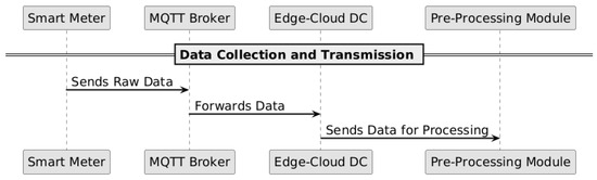
Figure 1. Data collection and transmission from smart meter to the cloud.

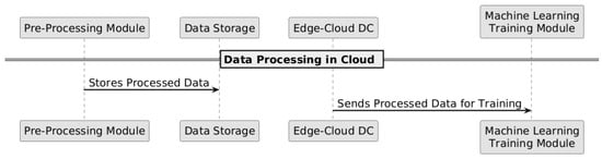
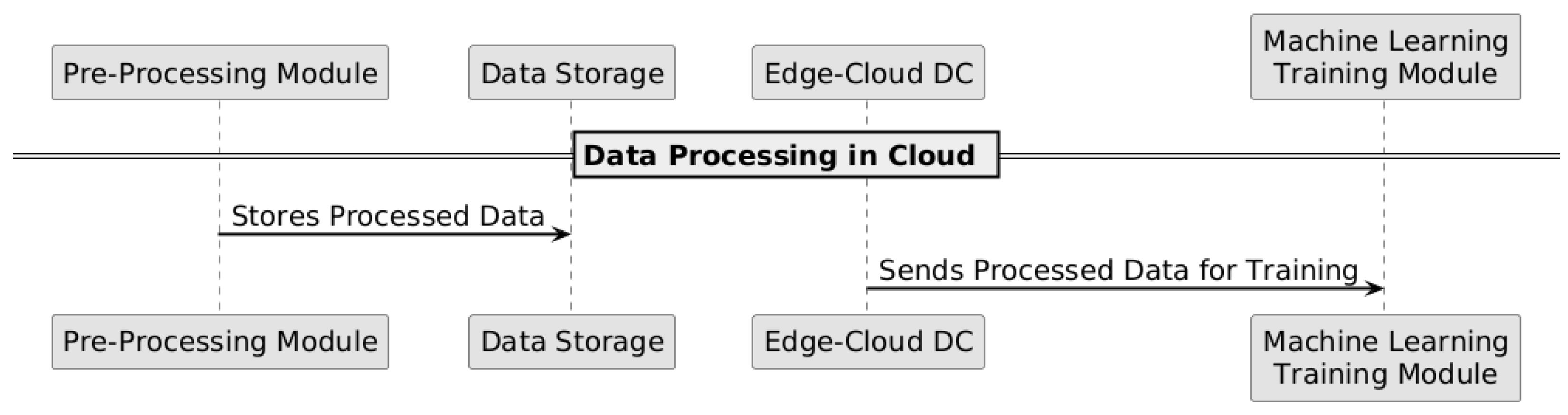
Figure 2. Data processing in the cloud for training machine learning models.

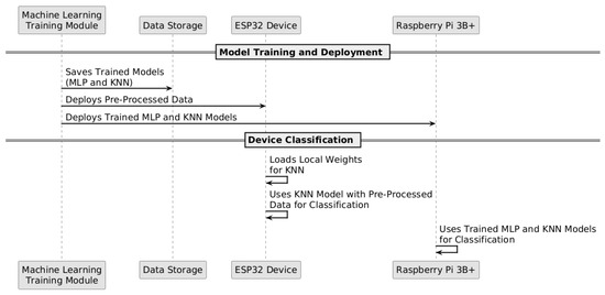
Figure 3. Deployment of trained models on extreme-edge devices.

The communication between the smart meter and the data acquisition module uses the MQTT protocol, enabling efficient data transmission to the cloud, as illustrated in Figure 1. This network connectivity is established through a layered architecture where edge devices connect to the cloud infrastructure as detailed in our IAIoSGT architecture. Figure 3 specifically demonstrates how trained models are deployed to extreme-edge devices, ensuring that the processed data stored in the cloud can be utilized for model training and subsequent deployment while maintaining computational efficiency at the edge.

3.2. Acquisition of Fundamental Signals

The fundamental voltage and current signals were captured using a smart meter developed by the authors of this work [23]. By utilizing the readings from this smart meter, we could record the sinusoidal voltage and current signals over time, allowing for an analysis of their behavior. Section 4 details the complete data acquisition process.

After acquisition, the raw signals are transmitted to the cloud via MQTT, where they undergo preprocessing steps, such as filtering and normalization. These transformations prepare the data for training the machine learning models (MLP and KNN). The complementary characteristics of these models justify their use: MLP generalizes well, handling complex patterns robustly, while KNN enables fast classifications with moderate resource consumption.

To optimize classification performance, the pre-trained MLP model, updated in the cloud, is utilized by the Raspberry Pi and deployed to the device. On the other hand, the ESP32 runs the KNN model locally, leveraging the ArduinoKNN library, where weights are reconfigured at each initialization to optimize the device’s limited resources.

Periodic synchronization ensures that both devices operate with updated models, enhancing classification accuracy. Although the goal is real-time classification, this initial approach validates the system’s architecture and operational feasibility.

3.3. Creation of Load Signature

This approach creates a unique load signature for each device using only its fundamental current signal. Instead of relying on multiple electrical parameters such as power, power factor, phase angle, or harmonics, the identification process focuses solely on the current signal and its amplitude variations in each cycle. This simplification reduces the need for complex processing, making identification more efficient and accessible without compromising accuracy. Additionally, by requiring fewer computational resources, this approach enables deployment on extreme-edge devices, allowing execution on hardware with limited resources, such as microcontrollers.

For example, in Figure 4, an example of the current behavior of devices over time can be observed, where unique characteristics can be used for differentiation.

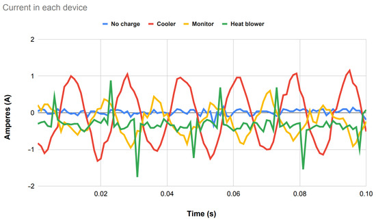
Figure 4. Fundamental current signal in each of the devices over time.

3.4. Main Modules

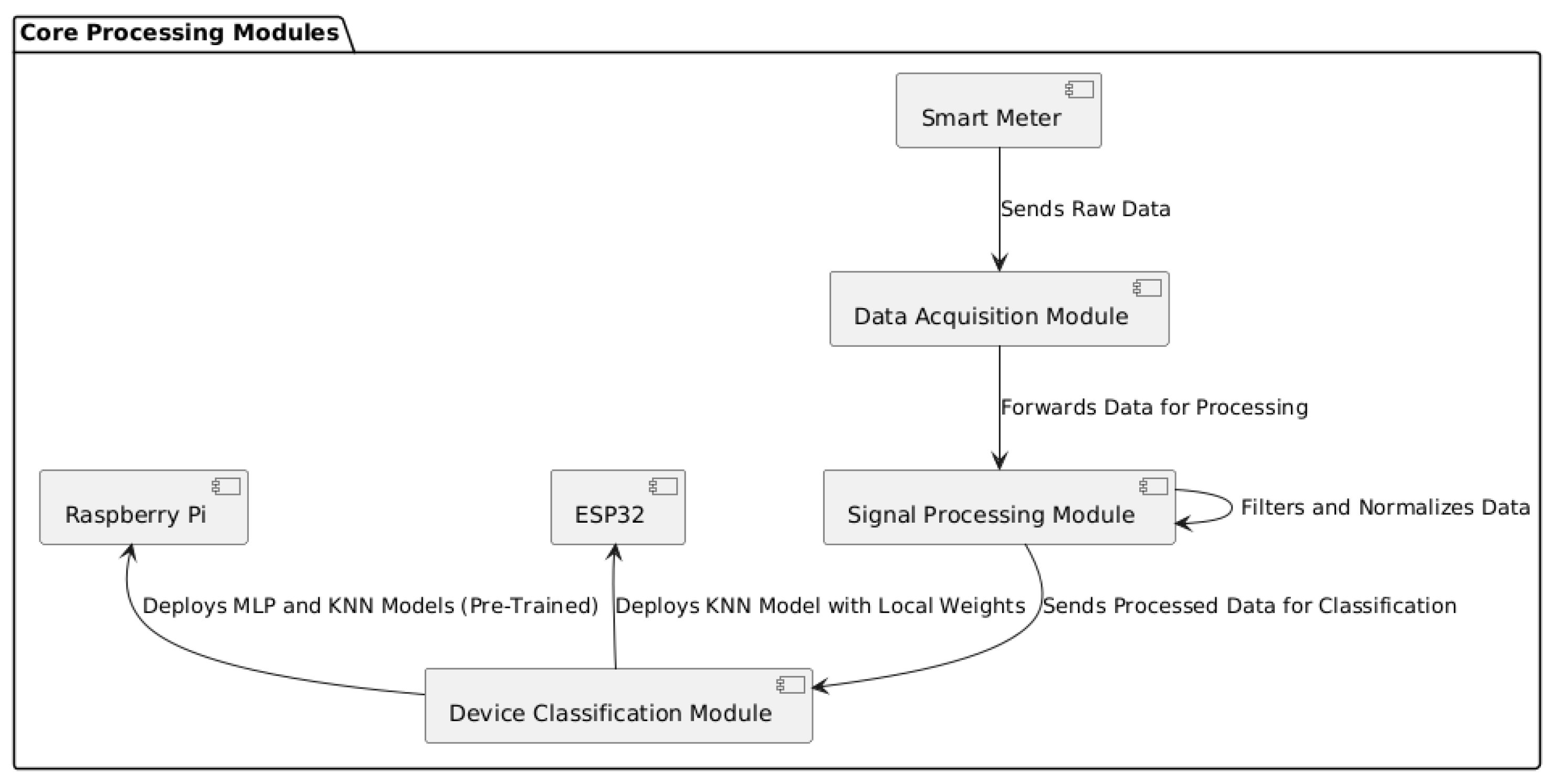
The system is composed of three main modules that work together to collect, process, and classify data from connected devices.

• Data Acquisition Module: Responsible for collecting voltage and current signals captured by the smart meter, which sends these raw data to the processing module via MQTT.
• Signal Processing Module: Located in the edge–cloud, it processes the raw data by applying filtering and normalization. The processed data are then stored and used to train machine learning models in the cloud.
• Device Classification Module: This module performs classification using MLP and KNN models. The pre-trained MLP and KNN models are directly applied on the Raspberry Pi, while, on the ESP32, the KNN model uses weights configured locally upon each initialization. Both devices receive preprocessed data from the cloud to ensure classification accuracy.

Figure 5 illustrates the data flow between the modules, highlighting the functions of each component in the processes of acquisition, processing, and classification.

Figure 5. Data flow in core modules for acquisition, processing, and classification.

4. Prototyping

The solution prototyping process is described in this section, addressing the steps involved in developing and validating the modules. It presents everything from defining an initial architecture and the definition of machine learning models to the methodology used in developing the solution. The methodology covers data acquisition to the final implementation of algorithms for identifying electronic devices. The main objective was to validate the effectiveness of the proposed modules in an extreme-edge environment, ensuring the viability and accuracy of the final solution.

4.1. IAIoSGT

The IAIoSGT (Artificial Intelligence in the IoSGT) is a software-driven edge–cloud architecture that integrates AI and ML into the Internet of Things for Smart Grids (IoSGT). This architecture comprises components collaborating to provide AI and ML capabilities in an edge–cloud environment. It facilitates automated processes in a continuous workflow, allowing for the collection and processing of data from smart devices. These data are used to train ML models that classify electronic devices.

The IAIoSGT is an extension of the IoSGT [24] that considers three main layers: extreme edge, edge–cloud DC, and central cloud DC. The architecture is configured to meet different requirements and needs. It is capable of collecting and processing data from smart sensors, making information available to applications or end users. This agility is enhanced by adopting open and standardized technologies, such as those provided by FIWARE, simplifying seamless integration with other platforms and systems. Furthermore, the architecture allows for real-time data analysis and automated decision-making.

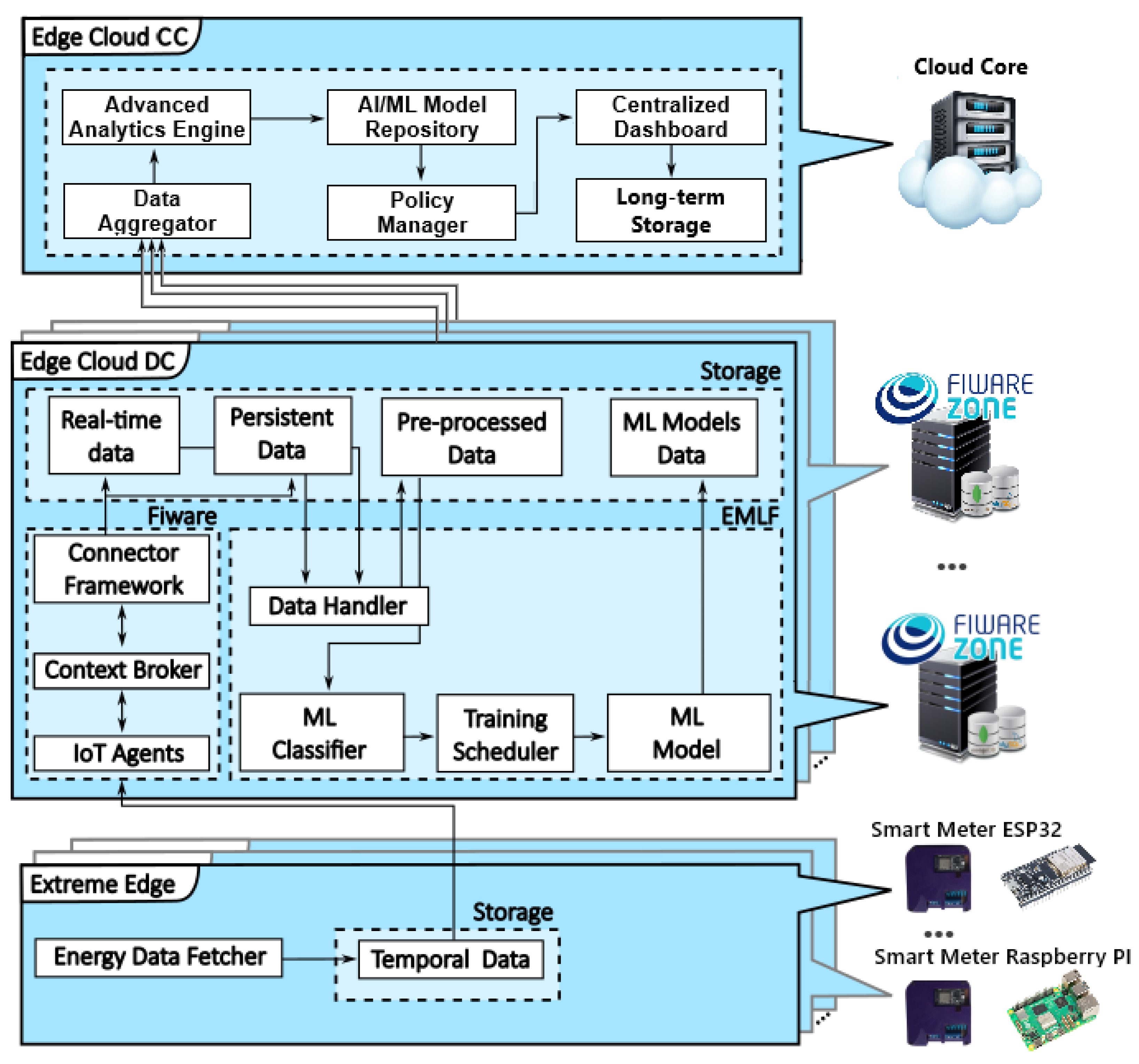
Figure 6 illustrates the IAIoSGT architecture, which is highly configurable and flexible, capable of adapting to meet different requirements and needs, including the implementation of ML and AI, making the platform useful for a variety of applications across different sectors. The architecture is divided into three main layers:

• Extreme Edge: This layer includes devices like smart meters equipped with microcontrollers such as the ESP32 or Raspberry Pi, which collect and preprocess data locally.
• Edge–Cloud DC: This layer handles data aggregation, ML model training, and real-time analytics. It includes modules like Eclipse Mosquitto, IOTA, Context Broker (Orion), and others.
• Central Cloud DC: Although not covered in this work, this layer would manage long-term storage and large-scale analytics.

The following sections will describe the function of each layer of the IAIoSGT, except the central cloud DC, which is outside the scope of this work.

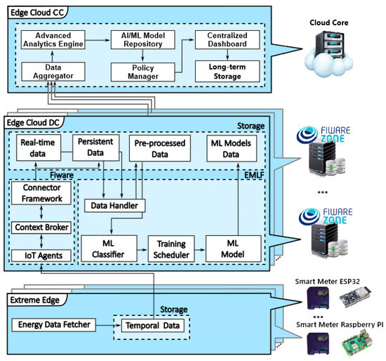
Figure 6. IAIoSGT architecture.

4.1.1. Edge–Cloud DC

The edge–cloud DC layer is modular and essential in managing SMs. It receives data from devices and applies ML and AI techniques, providing enriched information to SG managers. The edge–cloud infrastructure consists of eight modules: Eclipse Mosquitto 1.6.14, IOTA 1.20.0-distroless, Context Broker (Orion 3.5.1), Connector Framework (Cygnus 2.18.0), MySQL 5.7, MongoDB 4.4, EMLF, and Portainer. These modules are organized within the FIWARE ecosystem and encapsulated in Docker containers, which promotes scalability.

• Eclipse Mosquitto: A message broker that implements the MQTT protocol, facilitating communication between SMs and the edge–cloud layer.
• IOTA: Collaborates with Mosquitto to publish SM data to Orion.
• Context Broker (Orion): Centralizes and makes information available through an NGSI interface, allowing for contextual queries and local storage.
• Connector Framework (Cygnus): Includes contextual data in databases, automating the flow of information between modules. It uses MySQL for permanent storage and MongoDB for temporary data.
• EMLF: Uses Jupyter to process, classify, train, and make predictions from data generated by SMs, employing ML algorithms such as KNN and MLP.
• Portainer: Manages containers graphically, facilitating the administration and monitoring of the infrastructure.

The extreme-edge layer connects SMs simultaneously to edge–cloud DC through IOTA, which publishes the data to the Context Broker. Cygnus subscribes to the data for storage in MongoDB and MySQL, allowing for manipulation and analysis. After preprocessing, the data are classified and processed, resulting in valuable information for managing SG and optimizing system performance and efficiency.

4.1.2. Extreme Edge

The extreme-edge layer comprises intelligent electronic devices, which play a fundamental role in local data collection and processing, often in real time. In the context of this work, we used a smart meter with an ESP32 as its microcontroller.

The ESP32, developed by Espressif, is a highly versatile and powerful microcontroller. Its specifications include a 32-bit dual-core processor, integrated Wi-Fi and redtooth connectivity, and multiple input and output interfaces, such as ADCs and DACs. This microcontroller can perform complex tasks, such as executing machine learning models, making it an ideal choice for applications that require distributed processing and rapid response.

In addition to the ESP32, another example of a device that can be used in the extreme-edge layer is the Raspberry Pi. This device is a microprocessor and is also capable of executing ML models at the edge. In the current work, the Raspberry Pi 3B+ was used as a viable solution thanks to its 64-bit quad-core processor and 1 GB RAM capacity, allowing data processing and machine learning tasks to be performed locally without needing a constant connection to the cloud.

Two cases were used within the scope of this work: one using only the smart meter with the ESP32 as the central component, responsible for reading and processing energy data, as well as processing the AI. The other case uses a Raspberry Pi 3+ to process the AI through data received via serial communication from the smart meter. Notably, in this case, the ESP32 is used only to process energy data and send them via serial.

These devices, such as the ESP32 and Raspberry Pi 3+, demonstrate the capability to process and analyze data at the extreme-edge layer, offering efficient and autonomous solutions for real-time information collection and processing.

4.2. ML Models in Extreme-Edge Devices

In this section, we discuss the machine learning models (KNN and MLP) applied in this study. It is important to highlight that other methods and models were also studied, trained, and simulated to identify the best results for the application, as described in [1]. Based on the hardware limitations and performance constraints of the devices where the ML algorithms were implemented, only the KNN and MLP models were selected.

4.2.1. K-Nearest Neighbor (KNN)

K-Nearest Neighbor (KNN) [25] is an unparameterized and “lazy” supervised ML algorithm. The KNN algorithm considers the distance between the problem instances and a possible calculation object. Given an unlabeled instance, KNN adopts a voting-based strategy to select the K closest neighboring algorithms of that instance and chooses the label of the majority vote. The K-Nearest Neighbors are input to the algorithm, which uses the Euclidean distance to calculate the similarity of the instances. Simplicity and implementation flexibility are the main advantages of the KNN-supervised ML algorithm.

4.2.2. Multi Layer Perceptron (MLP)

Multi-Layer Perceptron (MLP) [26] is a class of fully connected artificial neural networks (ANNs) and is characterized by having one or more intermediate layers, which allows the treatment of complex and non-linear features [27]. The most used algorithm in MLPs is backpropagation, which injects a signal at the network’s input that propagates forward to the output layer. Then, the error is calculated, corresponding to the difference between the real and the result generated by the network. A signal sent to the previous layers calculates the new synaptic weights. The algorithm repeats until the error reaches a predefined value or a maximum number of repetitions [27].

4.3. Methodology

In this section, we present the methodology used in the development of this work. To evaluate the performance of the proposed system, we conducted two distinct experiments. In the first, the ESP32 microcontroller, preloaded with a CSV file containing previously captured energy reading samples, performed data classification using MLP and KNN algorithms, simulating an application at the extreme edge. In the second experiment, the ESP32 captured real-time energy data, stored them in a CSV file, and later made them available to a Raspberry Pi, which classified the parameters using the same algorithms. This second experiment enabled a comparative analysis of the algorithm performance on devices that can be deployed at the extreme edge.

All stages, from the acquisition of energy data to the final implementation on extreme-edge devices, are covered by the methodology. It includes manipulating and preparing the datasets, performing the preprocessing required to optimize the performance of the AI models, and implementing the devices specifically. Thus, it evaluates the effectiveness and efficiency of the different approaches tested.

4.3.1. Data Acquisition

Data collection was conducted in a controlled environment, starting with acquiring voltage and current data from electrical and electronic devices on a test bench. The collected data were organized and subjected to preprocessing, which used the “pandas.DataFrame.dropna()” filter to remove missing values. The methodology adopted for constructing this database was organized into successive steps, as detailed below:

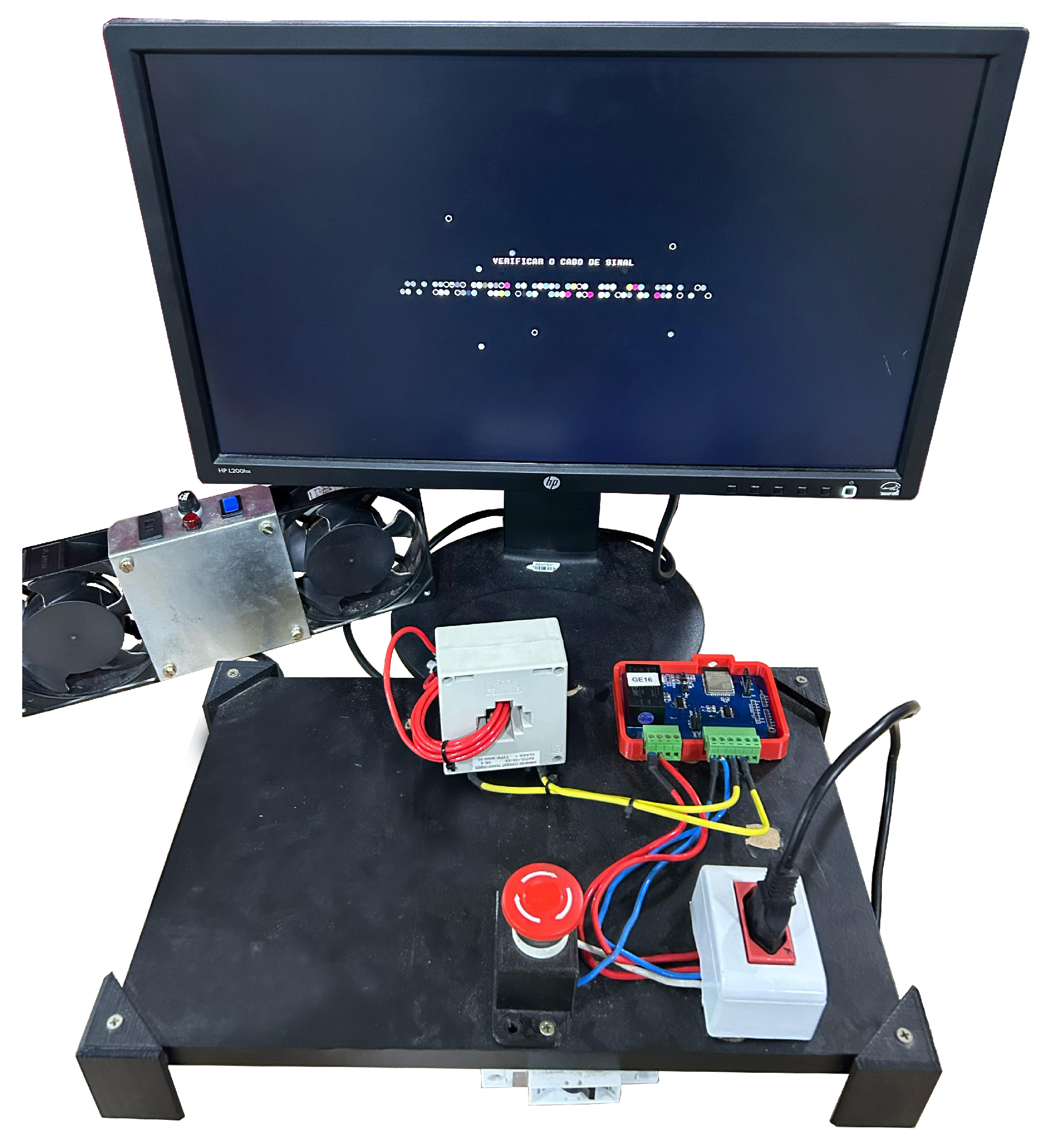
• Initially, three distinct devices (cooler, heat gun, and monitor) were added to the test bench (Figure 7), one at a time and individually, with the measurement of these devices being monitored and recorded by the SM. The devices were selected for their different energy consumption patterns and distinct current signatures.
  

  Figure 7. Testbed.
• Subsequently, the database for analysis was constructed. These datasets were created to identify the signature of each electrical and electronic device, highlighting its active consumption pattern in the electrical grid of a consumer unit. To achieve this, voltage, current, and power measurements were included and recorded over time, with samples collected at a granularity of 1 ms.
• A transpose matrix was applied to the data to enable the analysis of patterns in the sinusoidal forms of voltage and current signals, overcoming the limitation of point data. This adjustment ensured that each sample from distinct electronic devices contained 100 attributes of voltage, 100 of current, and 100 of power. Finally, the data from each electrical device were unified to form a comprehensive database, consolidating the information from all devices.

As previously mentioned, the dataset used in this research consists of voltage, current, and power measurements recorded over time, allowing the capture of information at various points of the sinusoidal wave. The main objective is to classify electrical and electronic devices based on their consumption signatures. To achieve this, the researchers considered four distinct environments as parameters: the first without load, in which no equipment is connected to the electrical grid, and the other three, each individually consisting of the respective electronic devices: coolers, monitors, and thermal blowers. In each case, the device was connected separately to the test bench, enabling exclusive and well-defined data collection for each signature.

It was decided to transpose the matrix of 100 temporal instances into a single one for better data visualization and signal processing. This way, a dataset with 300 attributes was obtained. Due to the environment used for data acquisition, four datasets were produced (one for data without load, one for the monitor, one for the thermal blower, and one for the cooler), each with 87 instances and 300 attributes. Furthermore, once the dataset was assembled, a filter was applied to shuffle the data, making the dataset random. This dataset was then named OriginalRAND.

To provide a clearer overview of the dataset used in this study, Table 1 summarizes the key features extracted from the acquired data. These features were used to classify the electrical and electronic devices based on their consumption signatures.

Table 1. Summary of key features extracted from the acquired dataset.

Dataset	Instances	Attributes
No Load	87	300
Monitor	87	300
Thermal Blower	87	300
Cooler	87	300

4.3.2. Dataset Manipulation and Preprocessing

The work was carried out with two datasets, as shown in Table 2, “OriginalRAND” and the reduced file “ProcessedRAND”, created from the original dataset, thus having a reduction in the number of rows. The original file contains 348 instances, while the “ProcessedRAND” file has 224 instances. The reduction in the number of instances was necessary to ensure that the dataset could be processed by the ESP32, which is used in this work and has a flash memory capacity of 4 megabytes.

Table 2. Summary of datasets used.

Database	Number of Instances	Number of Attributes
OriginalRAND	348	300
ProcessedRAND	224	300

The reduced dataset was used to run the KNN algorithm on the ESP32, where memory limitation was a constraint. This is useful for KNN and not for the MLP network. KNN is an instance-based algorithm that requires storing all training set examples since predictions depend on calculating the distances between new data points and stored examples. This process required a memory capacity not supported by the ESP32 used.

Thus, reducing the number of examples in the “ProcessedRAND” file was a crucial step in using KNN on the ESP32. This decision reflects a necessary trade-off between the amount of training data and the constraints imposed by the hardware environment. By adapting the dataset size to the available memory, it was possible to maintain the functionality of the KNN algorithm within the memory limits of the ESP32, ensuring that processing could be carried out efficiently without compromising the system’s execution.

Data preprocessing is crucial to ensuring the proper performance of the MLP and KNN algorithms, especially when considering performance tests with normalized and non-normalized data. The goal was to evaluate normalization’s impact on both models’ performance, particularly when the device’s hardware has limited resources.

Using the MLP, the data were organized into two scenarios: one using normalized data and the other with the original non-normalized data. Normalization was performed to ensure that all input variables were on the same scale, which is essential for the efficient operation of the MLP as it prevents variables with larger magnitudes from dominating the learning process. In the scenario with normalized data, the standard normalization technique was applied, where the features were adjusted to a distribution with a mean of zero and a standard deviation of one. We used the StandardScaler tool from the Scikit-learn library for this. In the second scenario, the data were used directly, without any transformation, to evaluate the impact of this lack of normalization on the training and final performance of the network.

Furthermore, the data were divided into three subsets: 70% for training, 20% for validation, and 10% for testing. This division aimed to optimize the MLP’s performance, ensuring its generalization capability. The performance was then evaluated based on the validation data, allowing for adjustments to the model parameters, and finally, it was tested on the dataset reserved for the final test.

Using the KNN algorithm on the ESP32, a more straightforward division was adopted, with the data being separated into training and testing sets, using 77% of the samples for training and 23% for testing. However, as with the MLP, tests were conducted with normalized and non-normalized data to compare the model’s performance in both scenarios. The same technique was used to normalize the MLP data. This process aimed to identify whether normalization, even in a simpler model like KNN, would improve performance, considering that the distance between points is the key metric for the algorithm’s operation. Although normalization is not strictly necessary for KNN, it can impact the result by preventing variables with higher magnitudes from distorting the calculated distances. When dealing with limited hardware, this could be considered a performance improvement.

5. Analysis of the Experiment Outcomes

The implementation of ML, KNN, and MLP models on extreme-edge devices is presented in this section. It will detail the implementation processes of these models on both the Raspberry Pi 3B+ and the ESP32 and analyze each device’s behavior and limitations when performing detection and classification tasks.

5.1. MLP Implementation

To find the optimal MLP neural network model, Keras Tuner 1.1.2 was used, a tool that allows efficient optimization of model hyperparameters. This approach aimed to test different network configurations, adjusting the number of layers, the number of units in each layer, and the learning rate to achieve the best possible performance with the input data.

The initial model was defined with multiple dense layers, testing variations in the number of units, ranging from 8 to 32, and the number of hidden layers, from 1 to 3, allowing the evaluation of the impact of model complexity on overall performance. The ReLU activation function was used in the hidden layers due to its robustness for deep networks. In contrast, the softmax function was applied in the output layer to handle multiclass classification. The model was compiled using the Adam optimizer, with learning rates of 0.01, 0.001, and 0.0001, which were tested to identify the optimal rate that maximized the network’s accuracy.

To efficiently explore the hyperparameter space, the Hyperband strategy was employed, limiting the maximum number of epochs to 50, aiming to balance training time and searching for more effective models. During this process, the model selection criterion was based on validation accuracy, and the early stopping technique was used to prevent overfitting and halting training when validation loss showed no improvement for five consecutive epochs.

Once the best model was identified, it was evaluated on the test dataset to measure its generalization capability. Following this step, the model was exported using TensorFlow Lite Micro 2.7.0, enabling its deployment on the ESP32. This conversion was essential to ensure the model could be implemented on embedded devices, preserving computational efficiency while maintaining the expected performance.

MLP HyperparameterSelection

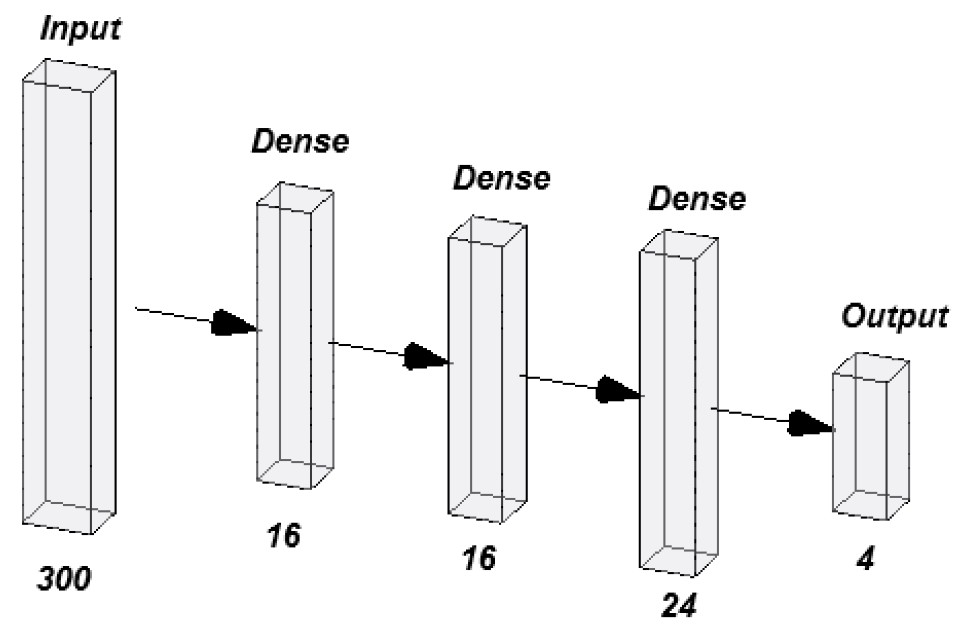
For the normalized dataset, the best-performing network consisted of three hidden layers. The first and second layers contained 16 neurons each, while the third layer had 24 neurons. The output layer consisted of 4 neurons, corresponding to the number of classes in the classification problem (Figure 8). This relatively simple configuration demonstrates that data normalization enabled the model to perform well with fewer neurons, making the network more computationally efficient.

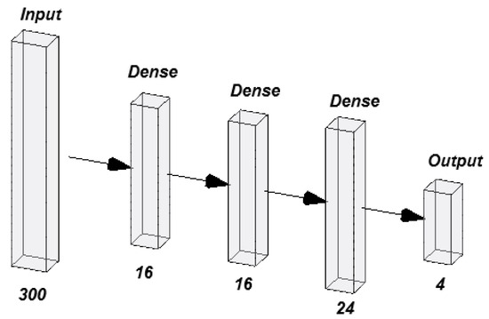
Figure 8. The best-performing MLP normalized.

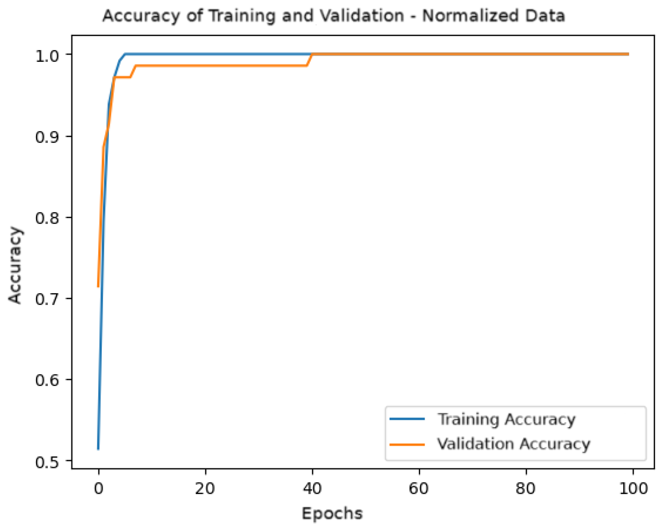
Figure 9 shows the accuracy graph during training and validation over the epochs. It is observed that both the training and validation accuracy quickly converge to values close to 1, indicating that the model effectively learned from the normalized data. From approximately 20 epochs onwards, the model exhibits stable accuracy without significant overfitting.

Figure 9. Training and validation accuracy for the model with normalized data.

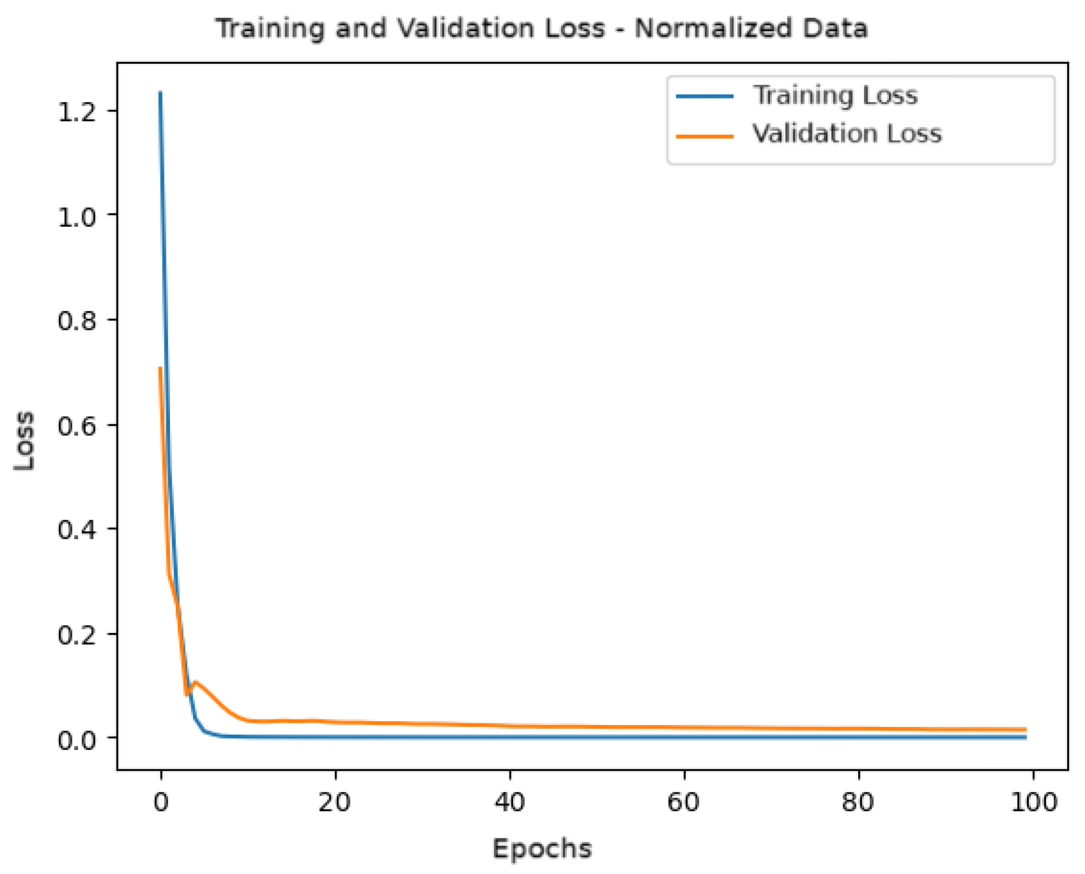
Figure 10 shows the behavior of the loss function during training and validation. A rapid convergence of the loss is observed in the first epochs, demonstrating that the model efficiently reduced the error. The validation loss closely follows the training loss, indicating that the model is generalizing well and is not suffering from overfitting.

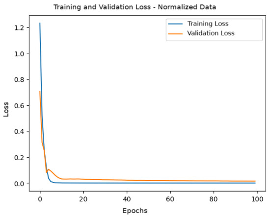
Figure 10. Training and validation loss for the model with normalized data.

The confusion matrix of the trained model, shown in Table 3, reveals that the model could classify most instances of each class correctly. All examples from the classes were classified correctly, achieving 100% accuracy. This highlights the model’s effectiveness in handling normalized data, with little to no confusion between classes.

Table 3. Confusion matrix for the model with normalized data.

	Predicted Labels
True Labels	No Load	Cooler	Blower	Monitor
No Load	13	0	0	0
Cooler	0	9	0	0
Blower	0	0	8	0
Monitor	0	0	0	5

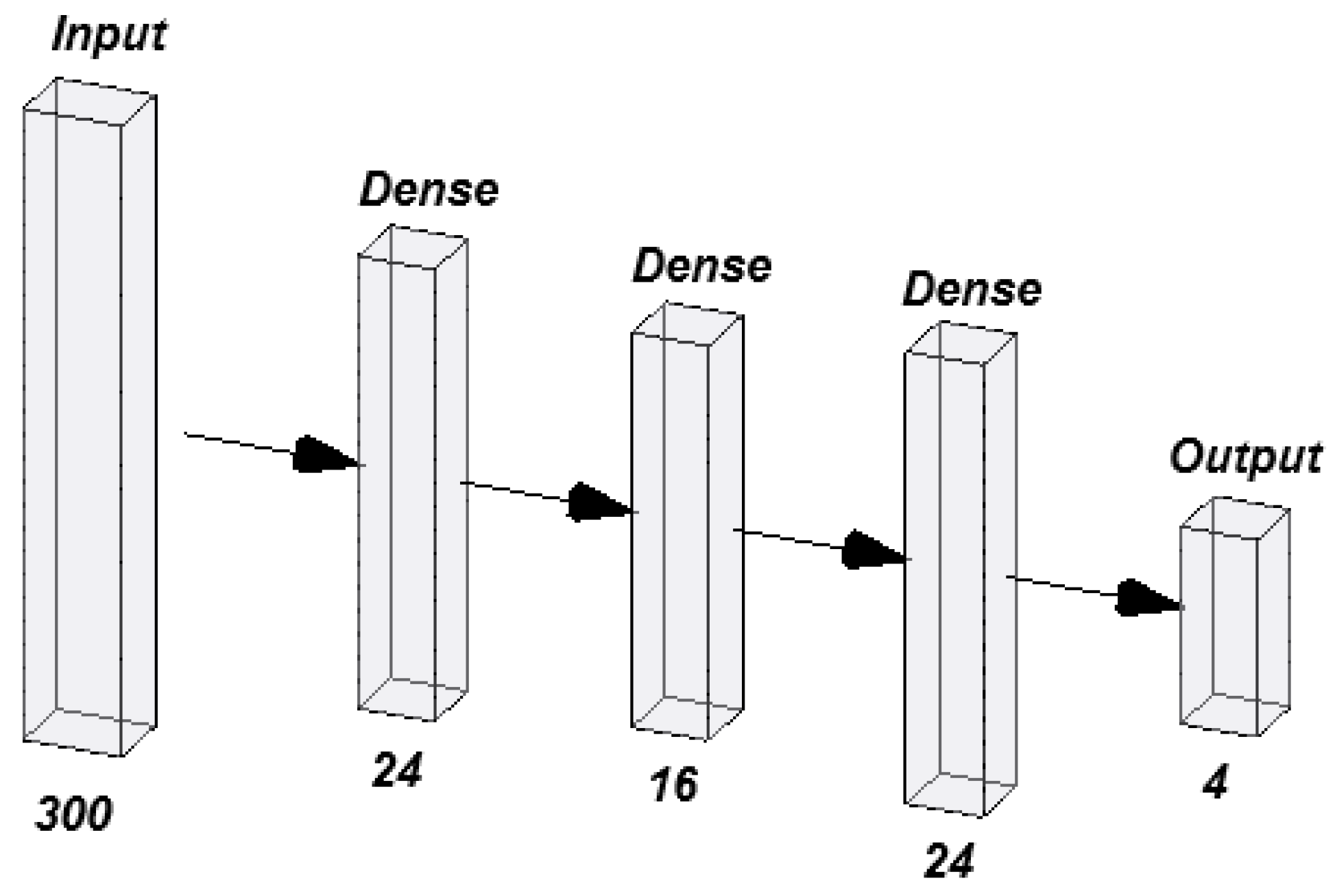
The optimized network presented a more complex architecture with three hidden layers when using the non-normalized dataset. The first layer consisted of 24 neurons, the second of 16 neurons, and the third again of 24 neurons. As in the previous model, the output layer also had 4 neurons (Figure 11). This more robust structure suggests that the network requires more capacity to capture the relationships between the input variables due to the greater variability in the non-normalized data.

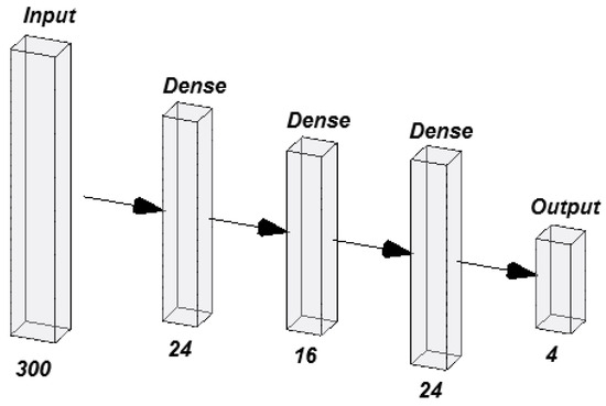
Figure 11. The best-performing MLP non-normalized.

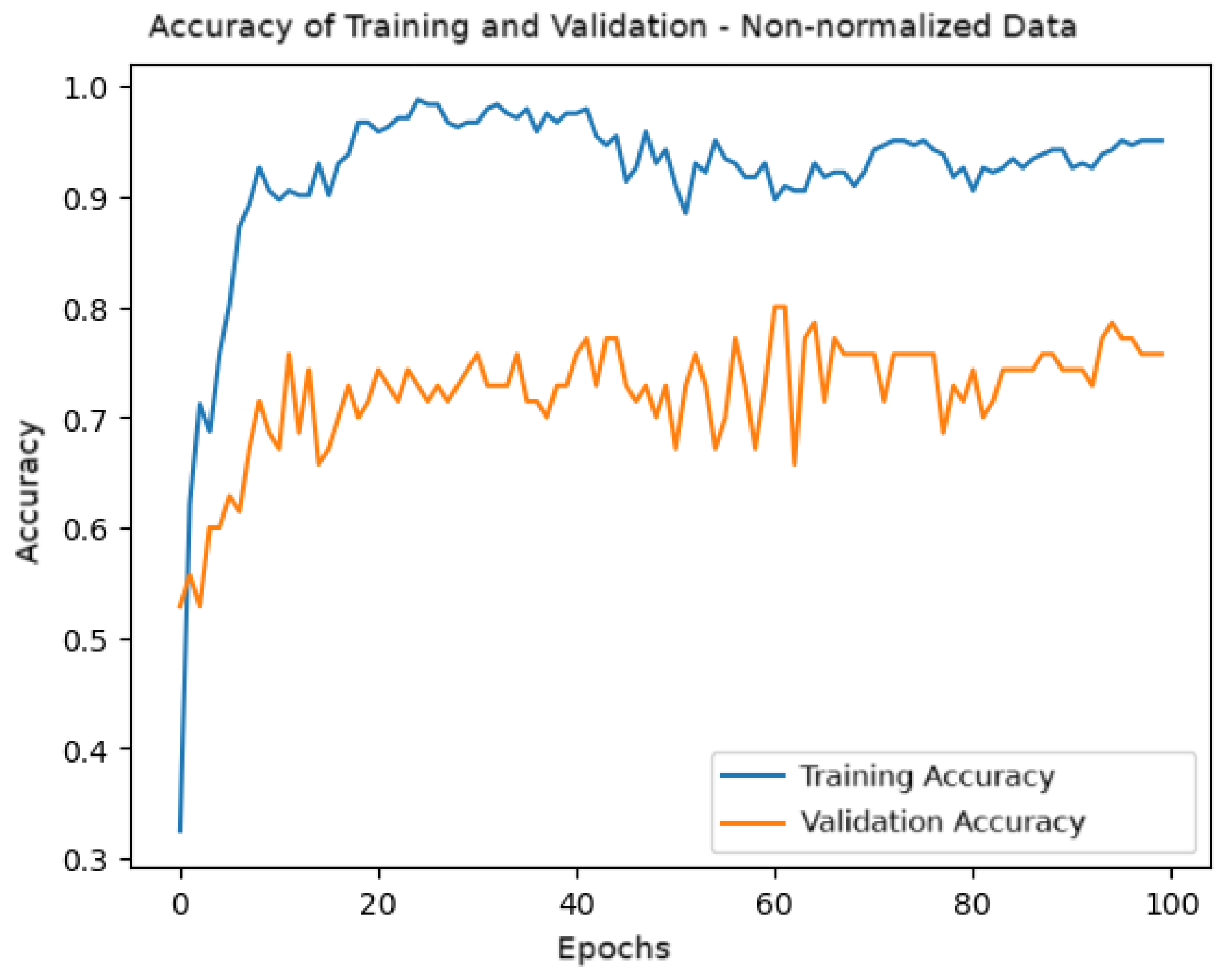
Figure 12 shows the accuracy graph during training and validation over the epochs. A higher variability in validation accuracy is observed compared to the normalized data, reflecting the model’s difficulty stabilizing learning with non-normalized data. The validation accuracy fluctuates around 0.7, while the training accuracy approaches 1.0, indicating a possible tendency for overfitting.

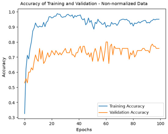
Figure 12. Training and validation accuracy for the model with non-normalized data.

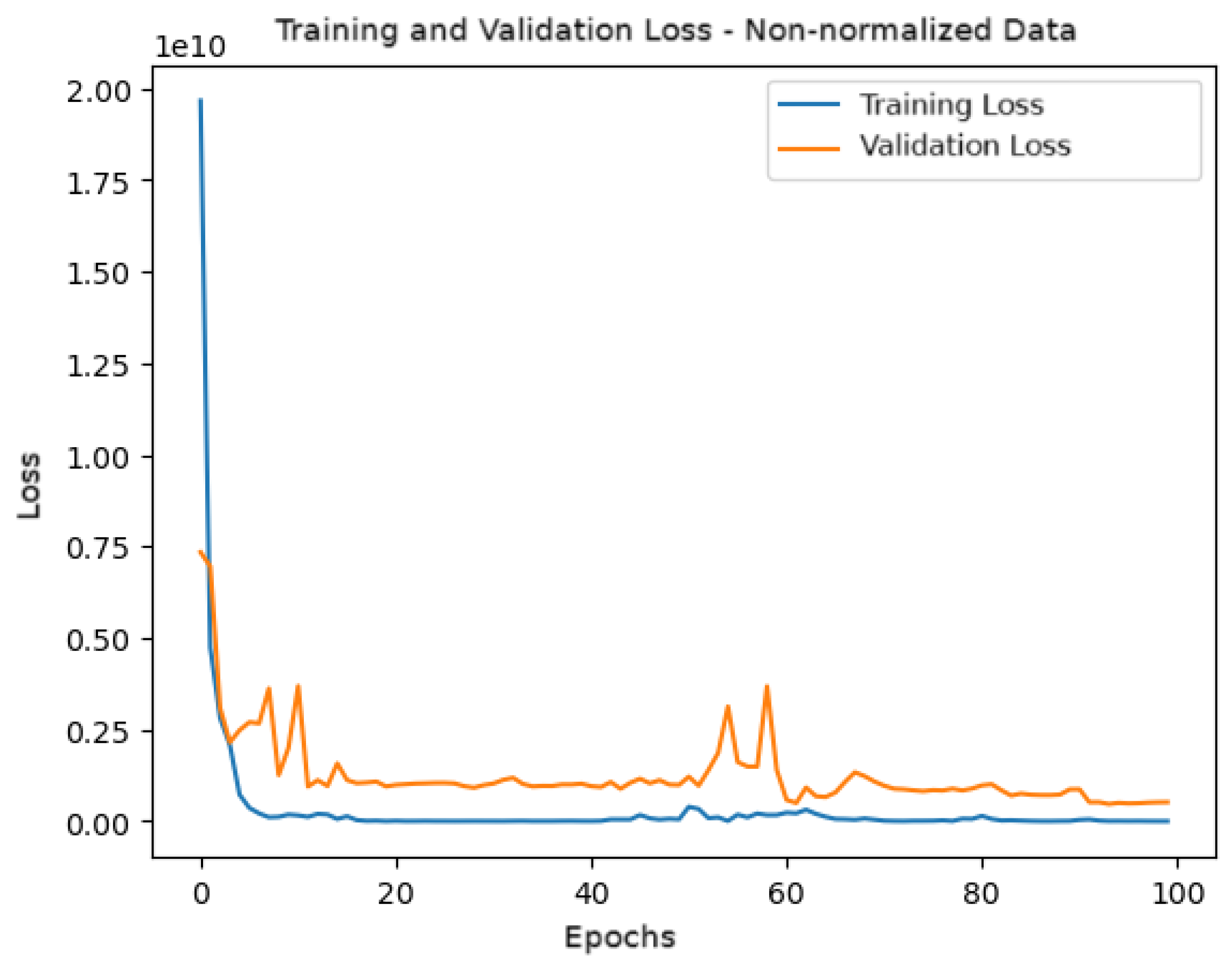
Figure 13 shows the behavior of the loss function during training and validation. It can be observed that the validation loss exhibits greater oscillations over the epochs, reinforcing the model’s difficulty in generalizing when the data are not normalized.

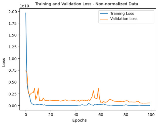
Figure 13. Training and validation loss for the model with non-normalized data.

The confusion matrix of the model, shown in Table 4, reveals that the model struggled to classify instances from the test set correctly. In particular, there is confusion between the classes, especially in classes 1 and 2, with several misclassified instances. This matrix confirms the model’s difficulty in handling variability in non-normalized data, emphasizing the importance of preprocessing techniques, such as normalization, to improve the network’s performance.

Table 4. Confusion matrix for the model with non-normalized data.

	Predicted Labels
True Labels	No Load	Cooler	Blower	Monitor
No Load	11	0	0	2
Cooler	4	5	0	0
Blower	0	2	5	1
Monitor	2	0	0	3

5.2. Quantitative Assessment of the Accuracy of Classification Models

Quantitative analysis was performed using metrics such as precision, recall, F1-score, and accuracy, enabling a detailed evaluation of the reliability of the classification methods employed. The results obtained for each model are presented below, considering two data preprocessing scenarios.

5.2.1. MLP Assessment

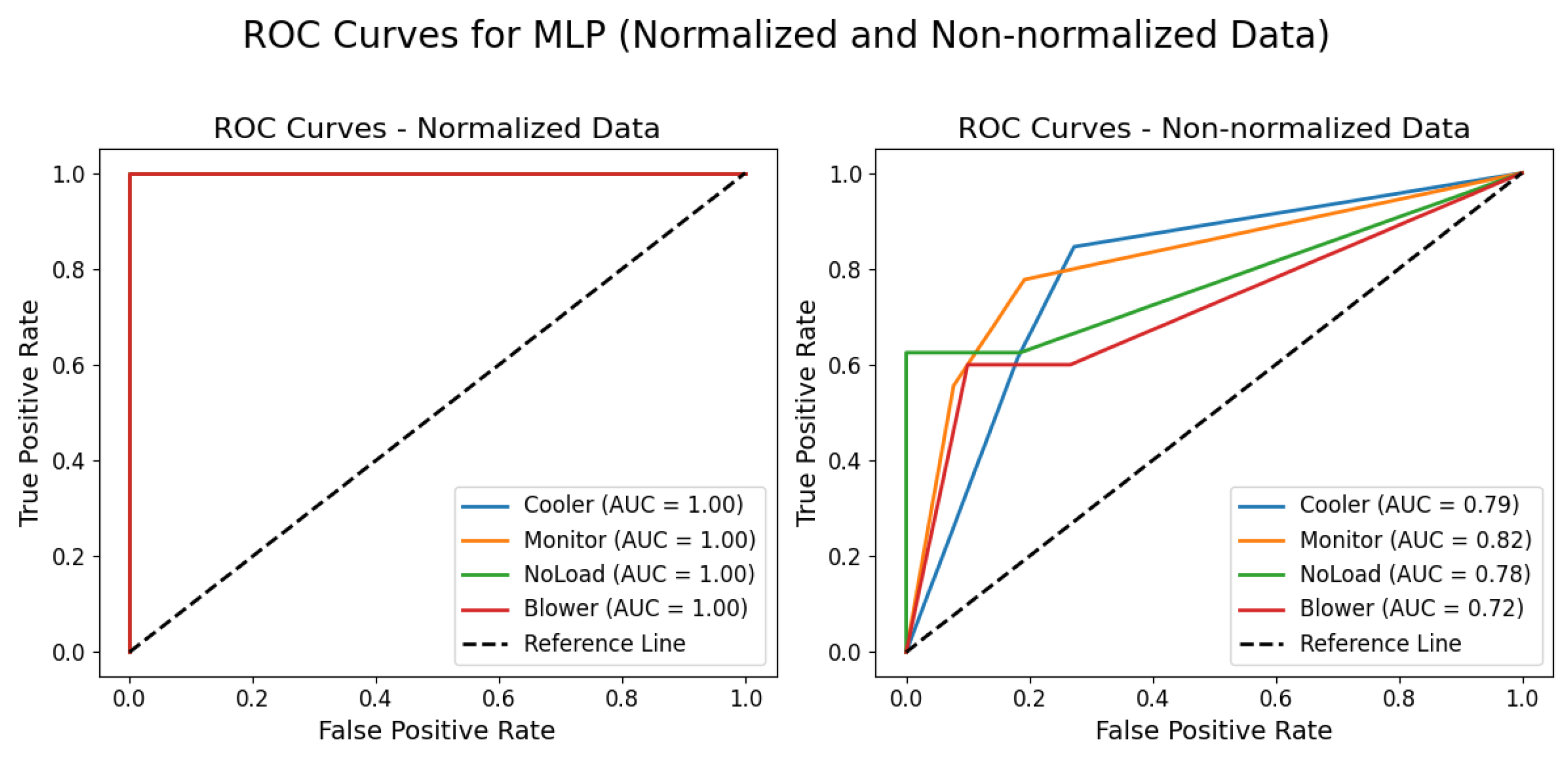
When the data were normalized, the MLP model showed ideal results, with all classes—cooler, monitor, no load, and blower—achieving precision, recall, and F1-score indices of 1.0, and an overall accuracy of 1.0. In contrast, the use of non-normalized data resulted in an overall accuracy of 0.69, revealing significant variations among the categories. For the cooler class, the precision was 0.65 and the recall was 0.85, indicating that, while a good proportion of examples were identified, there were a considerable number of false positives. In the monitor class, the values of 0.71 for precision and 0.56 for recall point to greater difficulty in retrieving the corresponding examples. The no load class achieved a perfect precision of 1.0; however, the recall of 0.62 shows that not all occurrences were captured, resulting in an F1-score of 0.77. Finally, the blower class exhibited the lowest indices, with a precision of 0.50 and a recall of 0.60, culminating in an F1-score of 0.55. Figure 14 illustrates the ROC curves obtained for the MLP model using both normalized and non-normalized data, further demonstrating the effect of data preprocessing on classification performance.

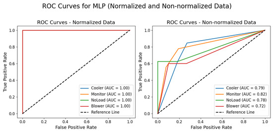
Figure 14. ROC curves for MLP with normalized and non-normalized data.

5.2.2. KNN Evaluation

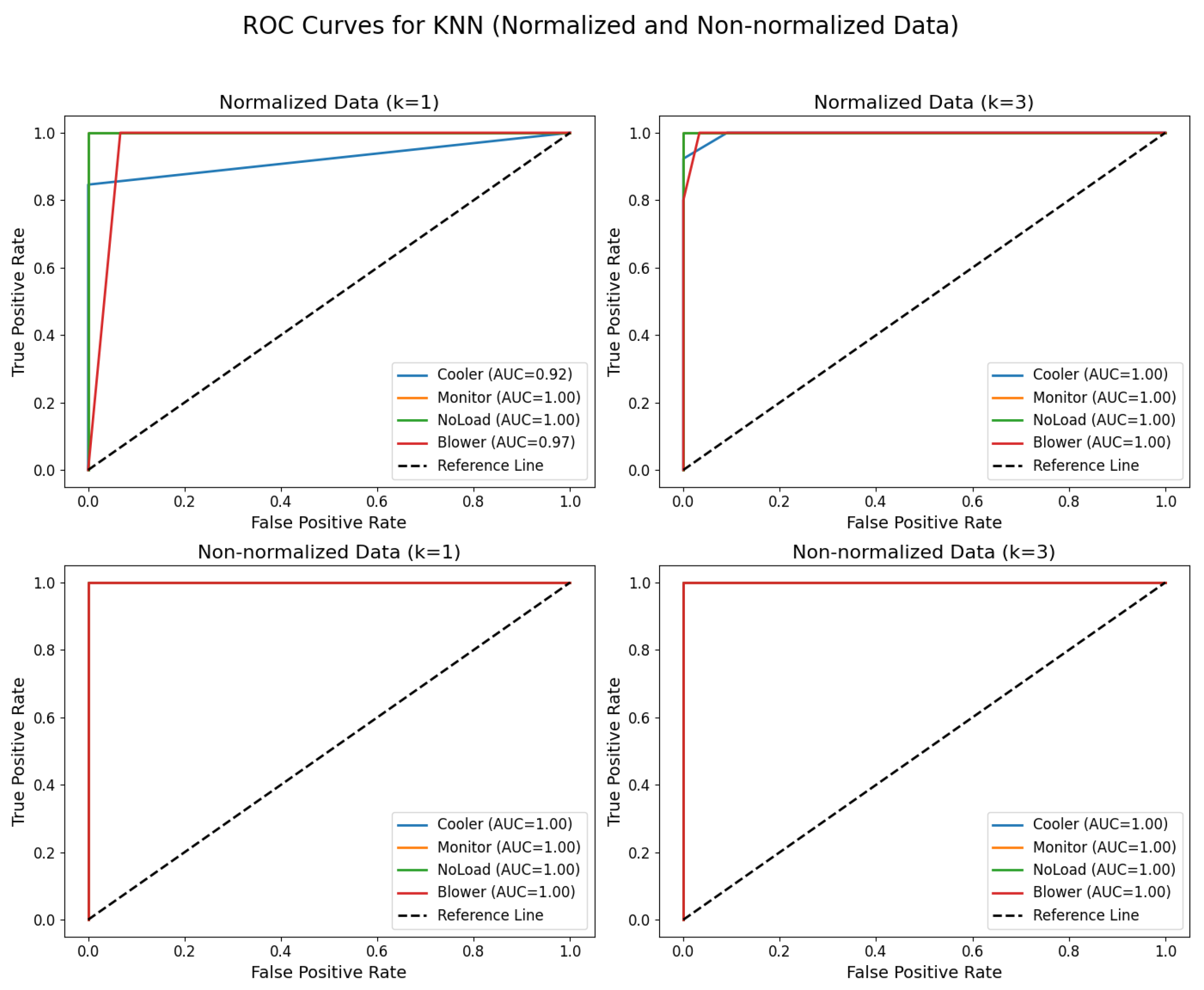
It was demonstrated by the experiments with the KNN algorithm that both the value of k and the preprocessing of the data significantly influence the classification results. Using normalized data, with $k=1$, an overall accuracy of 0.94 was achieved, where the cooler class had a precision of 1.00, recall of 0.85, and F1-score of 0.92; monitor recorded perfect metrics; no load also reached ideal indices; and blower had a precision of 0.71, although with a recall of 1.00 and an F1-score of 0.83. With $k=3$ and normalized data, the results were similar, maintaining an accuracy of 0.94, with the cooler class achieving a precision of 1.00, recall of 0.92, and F1-score of 0.96; monitor with a precision of 1.00, recall of 0.89, and F1-score of 0.94; no load with a precision of 0.89, recall of 1.00, and F1-score of 0.94; and blower with a precision of 0.83, recall of 1.00, and F1-score of 0.91. In contrast, the use of non-normalized data led to even more robust performance as, with both $k=1$ and $k=3$, the model achieved an accuracy of 1.00, with all classes—cooler, monitor, no load, and blower—exhibiting precision, recall, and F1-score equal to 1.00.

Figure 15 illustrates the ROC curves obtained for KNN using both normalized and non-normalized data, further reinforcing the impact of data preprocessing on classification performance.

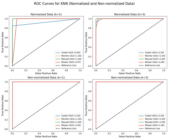
Figure 15. ROC curves for KNN with $k=1$ and $k=3$, using normalized and non-normalized data.

5.2.3. MLP on the Raspberry Pi 3B+

The Multi-Layer Perceptron (MLP) algorithm was trained on the IoSGT platform and subsequently imported to a Raspberry Pi. Model inference was performed in two distinct scenarios: with unprocessed data and with preprocessed data.

The best results were obtained with preprocessed data, as expected for an MLP. This occurs because data preprocessing, especially normalization, facilitates network learning by ensuring that weights are adjusted in a balanced and coherent manner across different input variables. As a result, the MLP was able to generalize the problem better, achieving higher accuracy and performance in the inference process, as shown in the confusion matrix in Table 5.

Table 5. Confusion matrix for MLP normalized data.

	Predicted Labels
True Labels	No Load	Cooler	Blower	Monitor
No Load	13	0	0	0
Cooler	0	9	0	0
Blower	0	0	8	0
Monitor	0	0	0	5

The model demonstrated excellent performance, achieving 100% accuracy in the conducted tests. This result indicates that the model was able to identify all instances correctly. Furthermore, the inference time was 93.80 ms using 3.9.2., and it was executed on the Raspbian operating system. This response time demonstrates the model’s efficiency, even in a more limited hardware environment like the Raspberry Pi. This performance also highlights the model’s ability to operate on low-cost systems without compromising accuracy or speed.

In the second scenario, without data preprocessing, as shown in the confusion matrix in Table 6, the MLP showed significantly lower accuracy, reaching only 37.14%. Additionally, the inference time was slower, taking 170.30 ms to complete execution. These results reinforce the importance of preprocessing, especially normalization, to improve the model’s accuracy and efficiency. The absence of preprocessing made it more difficult for the model to learn patterns in the data, resulting in accuracy far below expectations and an increase in inference time, likely due to the lack of standardization of variables.

Table 6. Confusion matrix of the MLP with un-normalized data.

	Predicted Labels
True Labels	No Load	Cooler	Blower	Monitor
No Load	4	2	7	0
Cooler	0	5	4	0
Blower	1	3	4	0
Monitor	0	0	5	0

5.2.4. MLP on ESP32

The implementation of the MLP neural network on the ESP32 was carried out using TensorFlow Lite Micro. Since the network’s architecture was relatively simple, quantization of the weights was not necessary when transferring the model to the microcontroller. This allowed for maintaining the expected accuracy without compromising efficiency. The network used 1936 bytes of memory for the model with normalized data and 1968 bytes for the model with non-normalized data, demonstrating the lightweight nature of the architecture employed.

When running the network with normalized data on the ESP32, an accuracy of 100% was achieved. The network successfully classified all instances in the test set, indicating that proper data preprocessing facilitated model generalization even in a hardware environment with limited resources.

The average execution time per prediction was approximately 0.31 milliseconds, showcasing the network’s high efficiency on the device. The combination of a simple architecture and data normalization was crucial in achieving this level of performance, both in terms of accuracy and temporal efficiency.

For the non-normalized data, the network exhibited lower accuracy, achieving 68.57%. The absence of normalization affected the network’s ability to correctly generalize patterns in the data, resulting in more incorrect predictions, especially among classes with more similar characteristics.

The average execution time per prediction was slightly higher, around 0.4 milliseconds. Although the network maintained good temporal efficiency, the lack of normalization significantly compromised the accuracy and reliability of the model, leading to confusion, primarily among the classes “cooler”, “blower”, and “monitor”.

5.3. Implementing K-Nearest Neighbors

In the experiment conducted with the KNN algorithm, two datasets were used: one previously normalized and another not. The data were divided into independent variables and the target variable, with normalization performed using the StandardScaler() function, ensuring that the independent variables were standardized to have a mean of zero and a standard deviation of one.

After this, the dataset was partitioned into training and testing data, with 80% allocated for training and 20% for testing, using train_test_split() with a randomization seed (random_state=30). For the implementation and performance testing of the best value of k for classification, the Scikit-learn library was utilized with the KNeighborsClassifier functionality. A loop was executed to test values of k ranging from 1 to 9, incrementing by two after each test.

5.3.1. KNN on Raspberry Pi 3B+

The experiment systematically evaluated different values of k (k = 1, k = 3, k = 5, and k = 7) and two types of weighting schemes (uniform and distance-based) in the KNN classifier. The goal was to assess the impact of these parameters on the model’s classification performance and computational efficiency.

For each configuration, the model’s accuracy was measured on the test set to determine how well it classified new data points. Additionally, the execution times for both training and prediction were recorded, providing insights into the computational costs associated with different values of k and weighting strategies.

To further analyze the model’s effectiveness, confusion matrices were generated for each tested configuration. These matrices provided a visual representation of how well the model distinguished between different classes, highlighting correctly classified instances as well as misclassifications. This allowed for a deeper evaluation of the classifier’s strengths and potential weaknesses.

Table 7 presents the confusion matrix for the KNN algorithm with K = 1, applied to non-normalized data. The results clearly demonstrate the model’s performance, with only a single instance being misclassified. This suggests that, for this specific dataset and preprocessing condition, KNN with k = 1 achieved high accuracy. However, further analysis is required to determine the stability of this performance across different parameter settings and data distributions.

Table 7. Confusion matrix for KNN (K = 1) non-normalized data.

	Predicted Labels
True Labels	No Load	Cooler	Blower	Monitor
No Load	12	0	0	1
Cooler	0	14	0	0
Blower	0	0	13	0
Monitor	0	0	0	12

The best results were obtained with K = 1 and K = 3, achieving respective accuracies of 100% and 94.87% for normalized data and 100% and 99.41% for non-normalized data. Regarding inference time, K = 3 showed the best performance in both scenarios, with 2.9 ms for normalized data and 4.38 ms for data without normalization. These results indicate that, although normalization improved inference time, data without preprocessing also achieved high accuracies, especially with K = 1. However, normalization allowed for more efficient execution, proving beneficial in balancing accuracy and response time.

5.3.2. KNN on the ESP32

For implementing the KNN algorithm on the ESP32, the Arduino_KNN library was designed to operate on devices with limited computational resources. The KNN classifier was set up to store up to 300 features per sample, and different values of k were tested, including 1, 3, 5, 7, and 9, to identify the value of k, providing the best accuracy in classifications.

The training and testing data were loaded from the SPIFFS file system directly onto the ESP32. Each data line consisted of up to 300 features followed by the corresponding label for the sample, which represented one of four categories: “no load”, “cooler”, “blower”, or “monitor”. During training, samples were added to the KNN classifier, which stored the features associated with their respective classes.

KNN classified the test examples for the testing phase by comparing the predicted labels with the actual ones. The algorithm’s performance was measured based on the accuracy of the predictions and the prediction time, accurately calculated using the esp_timer library. These prediction times were reported in milliseconds, allowing a clear assessment of the model’s efficiency on the ESP32.

In addition to accuracy, a confusion matrix was constructed for each value of K to visualize the rates of correct and incorrect classifications for each class. This provided a more detailed view of KNN’s performance, showing how the algorithm behaved for each type of load.

With the normalized data, accuracy varied according to the value of k, with the best accuracy observed for k = 1 and k = 3, both achieving 77.42%. As the value of k increased, accuracy decreased, dropping to 58.06% for k = 7 and 51.61% for k = 9. These results indicate that smaller values of k were more effective for the normalized dataset, but there was still considerable confusion between the classes.

In Table 8, the confusion matrix for k = 1 shows that the classes “cooler” and “blower” were frequently confused. The class “no load” was correctly identified in all instances. In Table 9, which presents the confusion matrix for k = 3, a similar pattern of confusion between the classes “cooler” and “monitor” is also noted.

Table 8. Confusion matrix for KNN (K = 1) with normalized data.

	Predicted Labels
True Labels	No Load	Cooler	Blower	Monitor
No Load	7	2	0	0
Cooler	0	6	1	1
Blower	0	1	4	0
Monitor	0	1	0	7

Table 9. Confusion matrix for KNN (K = 3) with normalized data.

	Predicted Labels
True Labels	No Load	Cooler	Blower	Monitor
No Load	7	2	0	0
Cooler	0	7	1	0
Blower	1	0	4	0
Monitor	0	2	0	6

Table 10 shows the confusion matrix for k = 1, where all instances of the classes “no-load” and “blower” were correctly classified, with only minor confusion observed in the “cooler” class. The performance was much more consistent compared to the normalized data. The average prediction time for the non-normalized data was slightly higher, ranging from 4.21 ms to 4.30 ms—times that can be considered acceptable given the limited hardware of the ESP32.

Table 10. Confusion matrix for KNN (K = 1) with non-normalized data.

	Predicted Labels
True Labels	No Load	Cooler	Blower	Monitor
No Load	13	0	0	0
Cooler	0	12	1	0
Blower	0	0	12	0
Monitor	0	0	0	14

The average prediction time for the normalized data was approximately 2.88 ms for k = 1, gradually increasing to 2.95 ms for k = 9 (as shown in Table 11). This demonstrates that, while KNN has good temporal efficiency on the ESP32, accuracy was limited for normalized data, suggesting that this preprocessing may not have been the most suitable for this scenario.

Table 11. KNN and MLP performance on ESP32 and Raspberry Pi 3B+ for normalized and non-normalized data.

Device	Data	Method	K	Accuracy (%)	Time (ms)
ESP32	Normalized	KNN	1	77.42	2.88
		KNN	3	77.42	2.90
		MLP	-	100	0.31
	Non-Normalized	KNN	1	96.23	4.21
		KNN	3	88.68	4.23
		MLP	-	68.57	0.40
Raspberry Pi 3B+	Normalized	KNN	1	100	18.72
		KNN	3	94.87	2.90
		MLP	-	100	93.80
	Non-Normalized	KNN	1	100	23.59
		KNN	3	99.41	4.38
		MLP	-	37.14	170.30

For the non-normalized data, KNN demonstrated significantly better results in terms of accuracy, achieving 96.23% for k = 1. As the value of k increased, accuracy gradually decreased, reaching 71.70% for k = 9. These results suggest that, unlike what is often observed in neural networks, KNN benefited from retaining the characteristics of the non-normalized data, which may have helped the model to identify more robust patterns.

6. Conclusions and Future Work

When the KNN and MLP algorithms were analyzed on limited hardware, it was found that the normalization process was crucial to achieving high performance when using the MLP, reaching 100% accuracy with an average prediction time of approximately 0.31 milliseconds. However, to use MLP on a device such as the ESP32, it will be necessary to perform data normalization before inserting it into the network, which consumes processing resources. This may be a limitation in applications that require real-time responses.

When analyzing the performance of the KNN algorithm, it showed better performance with non-normalized data, achieving up to 96.23% accuracy for k = 1. This information is relevant because it eliminates the need for data preprocessing, saving execution time and microcontroller processing in a real application. However, KNN requires storing the entire training dataset in memory, in addition to the test data, which may be unfeasible on devices with limited memory, such as the ESP32. In the specific case of this article, it was necessary to reduce the dataset to make the implementation viable.

Thus, we can observe that there is a trade-off between processing and memory when implementing these algorithms. Although additional processing for normalization is required by the MLP, a compact model that occupies less memory resulted, which is more suitable when memory is a critical resource. KNN, on the other hand, by avoiding the cost of normalization, demands more memory to store training and test data, which may not be the best choice in systems with storage constraints.

Based on the experiments, it was possible to verify that KNN obtained better results on the Raspberry Pi, standing out in accuracy and inference time. The MLP, in turn, presented similar accuracy on both hardware platforms (Raspberry Pi and ESP32) but with a slight advantage on the ESP32 when using non-normalized data. However, the main difference observed between the two devices was in the inference time.

Although the Raspberry Pi has more powerful hardware in terms of processing and memory, its inference times are significantly higher than those of the ESP32 due to the operating system overhead. The Raspberry Pi runs a Linux-based system, such as Raspbian, which manages multiple processes simultaneously, consuming resources and introducing latency. In contrast, the ESP32 runs bare-metal firmware, allowing model inference to take top priority without significant resource competition.

Additionally, the choice in programming language directly impacts performance. On the Raspberry Pi, inference runs in Python, an interpreted language that adds execution overhead since it dynamically translates each instruction into machine code. In contrast, the ESP32 operates in C or C++, compiled languages that generate optimized code for direct hardware execution, eliminating interpretation overhead and making inference far more efficient.

Finally, resource management plays a crucial role. The Raspberry Pi runs multiple processes simultaneously, sharing the CPU and memory with other system tasks, which can cause inference delays. On the ESP32, execution is exclusively dedicated to inference, ensuring more predictable and efficient performance. Therefore, despite the Raspberry Pi’s greater processing power, selecting the right platform and execution environment is key to optimizing performance for embedded and IoT applications.

To enable large-scale implementation within an SG, the proposed approach can be integrated into the IAIoSGT architecture, in which AI and SM are combined to optimize the performance of the power grid. In this structure, inference is performed locally by extreme-edge devices, such as the ESP32, and only essential information is sent to network edge or cloud servers, reducing latency and communication load. Additionally, scalability and computational efficiency are improved by adopting a hybrid model, in which lightweight algorithms are used on embedded devices, while more robust models are employed at the network edge. Through this strategy, real-time detection of consumption patterns, identification of connected devices, and optimization of energy distribution are enabled, ensuring a more efficient and resilient operation of the SG, even in scenarios with connectivity and computational capacity constraints.

References

- Marques, L.; Eugênio, P.; Bastos, L.; Santos, H.; Rosário, D.; Nogueira, E.; Cerqueira, E.; Kreutz, M.; Neto, A. Analysis of Electrical Signals by Machine Learning for Classification of Individualized Electronics on the Internet of Smart Grid Things (IoSGT) architecture. J. Internet Serv. Appl. 2023, 14, 124–135. [Google Scholar] [CrossRef]
- Javaid, N.; Hafeez, G.; Iqbal, S.; Alrajeh, N.; Alabed, M.S.; Guizani, M. Energy efficient integration of renewable energy sources in the smart grid for demand side management. IEEE Access 2018, 6, 77077–77096. [Google Scholar] [CrossRef]
- Vasisht, P.; Ranjan, S.; Jadhav, R.J.; Rasal, P.R.; Nrip, N.K. Smart Grid Technology and Renewable Energy Systems. In Proceedings of the 2022 International Conference on Smart and Sustainable Technologies in Energy and Power Sectors (SSTEPS), Mahendragarh, India, 7–11 November 2022; pp. 145–148. [Google Scholar] [CrossRef]
- Aggarwal, G.; Al-Greer, M.; Packiaraj, M.J.C.T. Smart Grid and IoT for Sustainable Smart Cities: Potential, Applications and Future Research Directions. 2023. Available online: https://smartgrid.ieee.org/bulletins/november-2023/smart-grid-and-iot-for-sustainable-smart-cities-potential-applications-and-future-research-directions (accessed on 11 April 2025).
- Basu, M. How Thailand will Integrate Renewables and EVs into the Grid. 2019. Available online: https://govinsider.asia/intl-en/article/surat-tanterdtid-how-thailand-will-integrate-renewables-and-evs-into-the-grid (accessed on 8 April 2025).
- Gough, M.B.; Santos, S.F.; AlSkaif, T.; Javadi, M.S.; Castro, R.; Catalão, J.P.S. Preserving Privacy of Smart Meter Data in a Smart Grid Environment. IEEE Trans. Ind. Inform. 2022, 18, 707–718. [Google Scholar] [CrossRef]
- Hseiki, H.A.; El-Hajj, A.M.; Ajra, Y.O.; Hija, F.A.; Haidar, A.M. A Secure and Resilient Smart Energy Meter. IEEE Access 2024, 12, 3114–3125. [Google Scholar] [CrossRef]
- Jiménez-Castillo, G.; Tina, G.M.; Muñoz-Rodríguez, F.; Rus-Casas, C. Smart meters for the evaluation of self-consumption in zero energy buildings. In Proceedings of the 2019 10th International Renewable Energy Congress (IREC), Sousse, Tunisia, 26–28 March 2019; pp. 1–6. [Google Scholar] [CrossRef]
- Algarni, A.; Ahmad, Z.; Alaa Ala’Anzy, M. An Edge Computing-Based and Threat Behavior-Aware Smart Prioritization Framework for Cybersecurity Intrusion Detection and Prevention of IEDs in Smart Grids With Integration of Modified LGBM and One Class-SVM Models. IEEE Access 2024, 12, 104948–104963. [Google Scholar] [CrossRef]
- de Freitas Velozo, L.; Mota, L.T.M. Bases de dados para Monitoramento Não-intrusivo da Carga: Uma revisão. In Proceedings of the Anais do Brazilian Technology Symposium (BTSym’22), Campinas, Brazil, 24–26 October 2022. [Google Scholar]
- Pereira, L.; Nunes, N. Performance evaluation in non-intrusive load monitoring: Datasets, metrics, and tools—A review. In Wiley Interdisciplinary Reviews: Data Mining and Knowledge Discovery; Wiley: Hoboken, NJ, USA, 2018; Volume 8, p. e1265. [Google Scholar]
- Quek, Y.; Woo, W.L.; Logenthiran, T. DC equipment identification using K-means clustering and kNN classification techniques. In Proceedings of the 2016 IEEE Region 10 Conference (TENCON), Singapore, 22–25 November 2016; IEEE: Piscataway, NJ, USA, 2016; pp. 777–780. [Google Scholar]
- Huang, S.J.; Hsieh, C.T.; Kuo, L.C.; Lin, C.W.; Chang, C.W.; Fang, S.A. Classification of home appliance electricity consumption using power signature and harmonic features. In Proceedings of the 2011 IEEE Ninth International Conference on Power Electronics and Drive Systems, Singapore, 5–8 December 2011; IEEE: Piscataway, NJ, USA, 2011; pp. 596–599. [Google Scholar]
- Qu, L.; Kong, Y.; Li, M.; Dong, W.; Zhang, F.; Zou, H. A residual convolutional neural network with multi-block for appliance recognition in non-intrusive load identification. Energy Build. 2023, 281, 112749. [Google Scholar] [CrossRef]
- Aslan, M.; Zurel, E.N. An efficient hybrid model for appliances classification based on time series features. Energy Build. 2022, 266, 112087. [Google Scholar] [CrossRef]
- De Baets, L.; Develder, C.; Dhaene, T.; Deschrijver, D. Detection of unidentified appliances in non-intrusive load monitoring using siamese neural networks. Int. J. Electr. Power Energy Syst. 2019, 104, 645–653. [Google Scholar] [CrossRef]
- Aghera, R.; Chilana, S.; Garg, V.; Reddy, R. A Deep Learning Technique using Low Sampling rate for residential Non Intrusive Load Monitoring. arXiv 2021, arXiv:2111.05120. [Google Scholar]
- Zim, M.Z.H. TinyML: Analysis of Xtensa LX6 microprocessor for Neural Network Applications by ESP32 SoC. arXiv 2021, arXiv:2106.10652. [Google Scholar]
- Orpa, T.H.; Ahnaf, A.; Ovi, T.B.; Rizu, M.I. An IoT Based Healthcare Solution With ESP32 Using Machine Learning Model. In Proceedings of the 2022 4th International Conference on Sustainable Technologies for Industry 4.0 (STI), Dhaka, Bangladesh, 17–18 December 2022; pp. 1–6. [Google Scholar] [CrossRef]
- Chen, Y.Y.; Lin, Y.H.; Kung, C.C.; Chung, M.H.; Yen, I.H. Design and Implementation of Cloud Analytics-Assisted Smart Power Meters Considering Advanced Artificial Intelligence as Edge Analytics in Demand-Side Management for Smart Homes. Sensors 2019, 19, 2047. [Google Scholar] [CrossRef]
- Balamurugan, M.; Narayanan, K.; Raghu, N.; Arjun Kumar, G.B.; Trupti, V.N. Role of artificial intelligence in smart grid—A mini review. Front. Artif. Intell. 2025, 8, 1551661. [Google Scholar] [CrossRef]
- Bastos, L.; Martins, B.; Santos, H.; Medeiros, I.; Eugênio, P.; Marques, L.; Rosário, D.; Nogueira, E.; Cerqueira, E.; Kreutz, M.; et al. Predictive Fraud Detection: An Intelligent Method for Internet of Smart Grid Things Systems. J. Internet Serv. Appl. 2023, 14, 160–176. [Google Scholar] [CrossRef]
- Sousa, E.L.d.; Marques, L.A.d.A.; Lima, I.d.S.F.d.; Neves, A.B.M.; Cunha, E.N.; Kreutz, M.E.; Neto, A.J.V. Development a Low-Cost Wireless Smart Meter with Power Quality Measurement for Smart Grid Applications. Sensors 2023, 23, 7210. [Google Scholar] [CrossRef] [PubMed]
- Santos, H.; Eugênio, P.; Marques, L.; Oliveira, H.; Rosário, D.; Nogueira, E.; Neto, A.; Cerqueira, E. Internet of Smart Grid Things (IoSGT): Prototyping a Real Cloud-Edge Testbed. In Proceedings of the 14th Brazilian Symposium on Ubiquitous and Pervasive Computing (SBCUP), Niterói, RS, Brazil, 31 July– 5 August 2022; pp. 111–120. [Google Scholar] [CrossRef]
- Altman, N.S. An Introduction to Kernel and Nearest-Neighbor Nonparametric Regression. Am. Stat. 1992, 46, 175–185. [Google Scholar] [CrossRef]
- Meyer-Baese, A.; Schmid, V. Chapter 7—Foundations of Neural Networks. In Pattern Recognition and Signal Analysis in Medical Imaging, 2nd ed.; Meyer-Baese, A., Schmid, V., Eds.; Academic Press: Oxford, UK, 2014; pp. 197–243. [Google Scholar] [CrossRef]
- Haykin, S. Redes Neurais: Princípios e Prática; Bookman Editora: Porto Alegre, Brazil, 2001. [Google Scholar]
Disclaimer/Publisher’s Note: The statements, opinions and data contained in all publications are solely those of the individual author(s) and contributor(s) and not of MDPI and/or the editor(s). MDPI and/or the editor(s) disclaim responsibility for any injury to people or property resulting from any ideas, methods, instructions or products referred to in the content. |
© 2025 by the authors. Licensee MDPI, Basel, Switzerland. This article is an open access article distributed under the terms and conditions of the Creative Commons Attribution (CC BY) license (https://creativecommons.org/licenses/by/4.0/).