1. Introduction
In Machine Learning, concept drift refers to the phenomenon of changing the distribution of instances of a specific problem over time [
1]. The causes of this phenomenon are varied, ranging from low representativeness of the set of instances used in the classifier’s training to changes in the environment in which the classifier operates [
2]. Several works present definitions for concept drift [
3,
4]. Among these, the definition proposed in [
3], summarized in Equation (
1), is widely accepted and stands out:
where
x is a feature vector
that describes an instance and
y represents a target variable.
represents the set of instances, while
is the set of target variables. A drift occurs at time
if the joint distribution (
) differs significantly from joint distribution (
) at time
. In [
5], it is stated that
j tends to infinity (
) in the context of data stream.
The concept drift problem can be analyzed based on two components: probabilistic sources [
3,
6,
7,
8,
9,
10,
11] and descriptors [
5,
12,
13,
14]. In the context of the probabilistic sources component, drifts are classified as virtual or real. In the first, the decision boundary between classes does not change. Consequently, there is no impact on the classifier’s performance. In the second, the decision boundary between classes changes, potentially impacting the classifier’s performance.
In terms of the second component, the descriptors of concept drift characterize the way a new concept replaces the current one. This characterization is based on properties such as the severity, influence zone, speed, frequency, recurrence, and predictability of the drift. According to the literature, this set of descriptors, detailed in
Section 2, defines the nature of concept drift [
13].
Taking into account that the occurrence of real concept drift can lead to degradation in classifier performance [
6], it is necessary to implement a reaction strategy when a drift is detected. Even though there are various possible reaction strategies, a common one is to generate a new base classifier and a new detector based on the latest instances. However, this strategy is not always suitable or feasible. For example, consider the scenario where labeling is costly and there exists a significant difference between the new concept and the current one. In this scenario, adopting the common reaction strategy can result in error higher than before the reaction, since there may be not enough instances to correctly learn the new concept, besides the high cost of labeling.
In the literature of concept drift, the topic of drift detection is widely addressed, whether from a supervised [
15,
16,
17,
18] or unsupervised [
7,
19,
20,
21,
22,
23] perspective. However, the adequacy of a reaction strategy is often overlooked. The study of the nature of concept drift can provide the necessary knowledge to define an appropriate reaction strategy. Nevertheless, very few works handle concept drift from the perspective of its nature.
In this context, this paper aims to analyze the impact of descriptors on concept drift. For this purpose, a comprehensive theoretical and experimental investigation was conducted. Experiments were performed on five synthetic datasets. Each dataset was simulated with 32 different combinations of descriptors. Considering that nine different contexts were tested in each dataset, we performed a total of 1440 tests. The results were analyzed and compared using statistical tests.
In summary, the contributions of this paper are as follows:
Empirical identification of relations between concept drift descriptors: Descriptors characterizing the same phenomenon naturally establish interrelationships. The analysis of these relationships provides critical insights into the phenomenon. This study identifies seven distinct relationships among the descriptors and classifiers, resulting in three groups based on their influence on classifier performance, descriptor behavior, and drift predictability. This contribution highlights the role of the interactions among descriptors in shaping concept drift.
Identification of descriptors with high and low impact on concept drift: The results of this research demonstrate that the characteristics of a drift affect the classifier’s performance in distinct ways. Thus, identifying which characteristics have the highest impact enables prioritizing them in the design of an evidence-based reaction strategy.
The rest of the paper is structured as follows.
Section 2 introduces concept drift descriptors;
Section 3 discusses related work; and
Section 4 describes the relationship between the descriptors identified in this paper. Then,
Section 5 presents the experiments conducted and the results obtained. Finally,
Section 6 concludes the paper and introduces future work.
5. Experiments and Results
The experiments were conducted to analyze the influence of the descriptors on concept drift by varying the values of each descriptor. To achieve this aim, five synthetic datasets in nine distinct contexts were investigated. First, six different drift detectors widely known in the literature were considered: two supervised DDM [
16] and EDDM [
17]; two semi-supervised DSDD [
23] and MD3-EGM [
19]; and two unsupervised DDAL [
54] and STUDD [
55]. Moreover, oracle versions of the supervised detectors were incorporated in the experiment (DDM-O and EDDM-O) in an attempt to evaluate the descriptors in a perfect drift detection environment. An oracle detector is an ideal detector that knows in advance all the drift points without loss, false, or detection delay. Finally, the ninth context considers no detection (ND), which is investigated to show the impact of descriptors when detection is not performed.
In terms of descriptor values, 32 variations were tested, here referred to as scenarios. Therefore, considering the five datasets and the nine detectors studied, a total of 160 distinct scenarios were investigated. A decision tree was used as the base classifier in all scenarios, with a total of 1440 different combinations analyzed. Finally, all detectors were applied using the default values defined by their authors.
The experiments were divided into two series, as summarized in
Figure 7. The first consisted of four stages and aimed to measure the performance of the classifier (C) in terms of prequential error, and the performance of the detector (D) regarding the percentage of false, missed, and detection delays. False detection was defined as a detection that occurs before a known drift; a missed detection occurred when a known drift was not detected; and a delayed detection was recorded when the detection occurred after a known drift, but was not characterized as a false detection. Then, the results from the first series were used as input for the second series of experiments. Two stages composed the second series, and the objective was to identify the combinations of descriptor values for concept drift that generated the best and the worst results considering the ranking of scenarios based on the median of prequential error. Both series were repeated for all nine contexts.
In the first stage of the first series of experiments, the performance metrics () of the detector were calculated for each of the 32 scenarios in the five datasets used. Likewise, the median prequential error () of the base classifier was calculated for each scenario in the second stage. In the third, the average of was calculated considering the medians of the prequential error for the same scenario i in each dataset. These averages formed a list of the classifier’s median performance in each scenario across each dataset. Finally, the list was sorted in ascending order. This list indicated in which scenarios the base classifier and the detector reached the best and the worst results.
The second series focused on statistical analysis of the results. The fifth stage divided the scenarios, ranked in the previous stage, by the values of the descriptors of each of the four analyzed descriptors. Then, in the sixth stage, the subgroups formed based on speed, severity, and recurrence were compared using the Mann–Whitney statistical test [
56], and the subgroups formed based on frequency were compared using the Friedman statistical test [
57]. In both tests, the significance level was set to
. In the end, the results indicated which value for each descriptor led to better or worse performance (
), as detailed in
Table 5.
The first column of
Table 5 indicates the scenario identifier. The second presents the detail of the drift in terms of descriptors in the following order: Speed-Severity-Recurrence-Frequency. The values for each descriptor are represented by their initials and are detailed in the footnote. Columns 3, 4, and 5 show information about drift: number of existing drifts, speed, and frequency. The presence of only one value indicates a periodic drift, while non-periodic drifts are signaled by “Alt”, with drift interval values shown in the footnote. To better illustrate, consider scenario 1 where drift is defined as (A) Abrupt, (H) High, (R) Recurrent, and (PH) Periodical High, for the speed, severity, recurrence, and frequency descriptors, respectively. In this scenario, there are 39 drifts, all with a speed set to 1 and occurring every 250 instances. Note that, to reduce space, each line represents two scenarios. The results obtained in our two series of experiments are discussed in
Section 5.3 and
Section 5.4.
5.1. Datasets
Real-world datasets have significant limitations when it comes to concept drift, particularly due to the difficulty of accurately identifying the location of drifts or confirming their existence. Additionally, only a few well-known datasets include verified concept drifts [
58,
59]. Approaches such as injecting drifts into real-world datasets are often restricted to modifying the speed descriptor [
60], which falls short of the objectives of this study, as it explores more complex descriptors such as speed, severity, frequency, and recurrence.
To overcome these limitations, synthetic datasets were employed in this paper because they allow the simulation of different types of drift by modifying instances, making it possible to understand how the descriptors impact drift. In this work, 32 variations were generated for each of the five synthetic datasets provided in [
12]: Line, Hyperplane, SineH, SineV, and Circle. Each dataset represents a binary classification problem with
balanced instances, without noise, and with two features, except for the Hyperplane dataset, which contains three features.
The Line and Hyperplane datasets are defined by
, where
and
for Line and Hyperplane, respectively. In our experiments, we varied the
values. SineH and SineV are defined by
. We varied the value of
b in SineH, affecting the horizontal axis, and the value of
c in SineV, affecting the vertical axis. Finally, the Circle dataset is defined by
, whose
r values were varied.
Table 5 summarizes the descriptors of the 32 generated scenarios for each dataset.
Additionally, for each synthetic dataset, specific parameters were adjusted to simulate different types of concept drift. For example, in the Line dataset, high-severity drifts were created by shifting the value of by for each concept, while for low-severity drifts, the values were shifted by . Similarly, in Circle, high-severity drifts were created by shifting the radius parameter (r) by for each new concept, while for low-severity drifts, the value was shifted by .
In all datasets, recurrence was simulated by repeating the concepts from the middle of the known drifts. The frequencies of concept drift were simulated by adjusting the intervals between their occurrences. For instance, in high-frequency scenarios, a drift occurs every 250 instances, whereas in low-frequency scenarios, they occur every 3000 instances. Lastly, abrupt drifts were simulated by replacing the current concept with a new one after a single instance, while gradual drifts were simulated by progressive replacement of concepts over 250 instances.
Table A1 provides a detailed summary of parameter adjustments used to represent the descriptor variations in each dataset.
5.3. First Series of Experiments
The results of the first series of experiments are summarized in
Figure 8. It is worth noting that the DDM-O, EDDM-O, and ND scenarios are not represented in this figure due to the following reasons: detection is perfect (oracle) in the first two; and there is no detection in the last one.
When considering supervised detectors, DDM and EDDM provided the lowest delay rates. However, DDM reached lost detection rates mostly higher than , as well as a high percentage of false detections, with some exceptions. In terms of EDDM, the percentage of lost detection does not follow an explicit pattern and depends on the scenario, while the false detection rate is usually lower than . In the unsupervised scenarios, surprisingly, DDAL and STUDD did not detect drift. Consequently, the percentages of false and delayed detections were zero, while lost detection was maximum. The performance of unsupervised detectors was, therefore, similar to the no-detection scenario. Finally, the two semi-supervised methods showed divergent results when compared to each other. On the one hand, MD3-EGM and DSDD had opposite lost detection performances. On the other, MD3-EGM achieved a lower delay detection rate, while DSDD reached a lower false detection rate.
The direct comparison among the six detectors indicates an order relation between them. DDM and EDDM performed the best, followed by DSDD and MD3-EGM. The worst were the unsupervised methods, since they did not detect any drift. This poor performance may be due to the values of the models’ hyperparameters. The success of unsupervised methods typically depends on fine-tuning several hyperparameters. However, in our experiments, the default values of the methods were used, without fine-tuning.
When analyzing the medians of the base classifier prequencial error in each context, shown in
Figure 9, DDM and MD3-EGM presented the worst performance, as indicated by their highest medians of prequential error in all datasets. Moreover, DDM-O also achieved a high error rate in the Circle dataset. The opposite results are observed for EDDM, which achieved the lowest median of error across all scenarios. This result is consistent with the false detection and delay rates obtained by EDDM (
Figure 8).
It is also important to compare the supervised detectors to their oracle versions in terms of prequential error. DDM-O outperformed DDM, except for on the Circle dataset. In turn, surprisingly, EDDM provided better or equal performance compared to EDDM-O. Finally, considering the context without detection, its performance was similar to those of the other contexts. This suggests that the best way to react to drift is not always to retrain the models. This observation is reinforced when we consider unsupervised methods, whose performances are similar to those observed in scenarios with no drift detection.
6. Conclusions and Future Work
In this study we analyzed the impact of four concept drift descriptors on the performance of base classifiers and drift detectors, intending to identify the most relevant descriptors for the drift reaction process. The experiments were conducted on five different datasets with 32 variations in descriptor values, eight different detectors, and a context without detection, totaling 1440 different combinations tested. The results indicated that concept drifts characterized by low speed, low severity, non-recurrence, and low periodicity generated smaller impacts on classifier performance. On the other hand, drifts with high speed (abrupt), high severity, recurrence, and high periodicity generated a higher impact on classifier performance.
Our first conclusion is that the reaction to concept drift cannot be uniform for all types of drift. Instead, it must consider the specific characteristics of each drift and, in some cases, it may be argued that the best response is simply not to react. When detailing the results shown in
Table 7, it was observed that speed, severity and recurrence presented well-defined values for the scenarios with better and worse performances, while frequency showed much less defined behavior. This suggests that the first three descriptors have the strongest influence on drift. However, by combining these results with those in
Table 6, it is observed that only the results of severity predominantly show significant differences, followed by frequency and recurrence.
The second conclusion is that severity, recurrence, and frequency provide, respectively, and in descending order, the strongest impacts on concept drift. It is worth noting that the isolated impact of severity appears to be higher than that of the other descriptors. Speed does not appear to have an impact on drift. Therefore, any reaction strategy must consider the descriptors with the strongest impact. Finally, our third conclusion is that there is a need to incorporate mechanisms allowing describing concept drift into the process designed to handle such a phenomenon. This mechanism can be executed concurrently with the detection process. Moreover, the properties provided by the description mechanism should be used to determine the more effective reaction strategy to be used.
Based on the aforementioned conclusions, we suggest that future research should address the analysis of the mutual impact of descriptors on concept drift, as well as delve deeper into the analysis of relationships between descriptors, develop mechanisms to characterize drift in terms of these descriptors, analyze the impacts of concept drift on deep learning models, and investigate how and if these impacts differ from those observed in shallow models. We also intend to investigate how the specific characteristics of real-world problems can impact the influence of descriptors on reaction strategies, and design detectors that consider the characteristics of drift.
Author Contributions
Conceptualization, A.C., R.G. and E.M.d.S.; Methodologies, A.C., R.G. and E.M.d.S., Formal analysis, A.C.; Investigation, A.C.; Software, A.C.; Writin—Original Draft, A.C., Writing—Review and Editing, A.C., R.G. and E.M.d.S.; Visualization, A.C., R.G. and E.M.d.S. All authors have read and agreed to the published version of the manuscript.
Funding
This study was financed in part by the Coordenação de Aperfeiçoamento de Pessoal de Nível Superior—Brasil (CAPES-PROEX)—Finance Code 001. This work was partially supported by Amazonas State Research Support Foundation—FAPEAM—through the POSGRAD project 2024/2025.
Institutional Review Board Statement
Not applicable.
Informed Consent Statement
Not applicable.
Data Availability Statement
Conflicts of Interest
The authors declare no conflicts of interest.
References
- Gemaque, R.N.; Costa, A.F.J.; Giusti, R.; dos Santos, E.M. An overview of unsupervised drift detection methods. WIREs Data Min. Knowl. Discov. 2020, 10, e1381. [Google Scholar] [CrossRef]
- Hinder, F.; Kummert, J.; Hammer, B. Explaining Concept Drift by Mean of Direction. In Proceedings of the Artificial Neural Networks and Machine Learning—ICANN, Bratislava, Slovakia, 15–18 September 2020; Farkaš, I., Masulli, P., Wermter, S., Eds.; Springer: Cham, Switzerland, 2020; pp. 379–390. [Google Scholar]
- Gama, J.; Žliobaitė, I.; Bifet, A.; Pechenizkiy, M.; Bouchachia, A. A Survey on Concept Drift Adaptation. ACM Comput. Surv. 2014, 46, 1–37. [Google Scholar] [CrossRef]
- Guo, H.; Li, H.; Ren, Q.; Wang, W. Concept drift type identification based on multi-sliding windows. Inf. Sci. 2022, 585, 1–23. [Google Scholar] [CrossRef]
- Lu, J.; Liu, A.; Dong, F.; Gu, F.; Gama, J.; Zhang, G. Learning under Concept Drift: A Review. IEEE Trans. Knowl. Data Eng. 2019, 31, 2346–2363. [Google Scholar] [CrossRef]
- Bayram, F.; Ahmed, B.S.; Kassler, A. From concept drift to model degradation: An overview on performance-aware drift detectors. Knowl.-Based Syst. 2022, 245, 108632. [Google Scholar] [CrossRef]
- Castellani, A.; Schmitt, S.; Hammer, B. Task-Sensitive Concept Drift Detector with Constraint Embedding. In Proceedings of the 2021 IEEE Symposium Series on Computational Intelligence (SSCI), Virtual, 5–7 December 2021; pp. 1–8. [Google Scholar] [CrossRef]
- Iwashita, A.S.; Papa, J.P. An Overview on Concept Drift Learning. IEEE Access 2019, 7, 1532–1547. [Google Scholar] [CrossRef]
- Yan, M.M.W. Accurate detecting concept drift in evolving data streams. ICT Express 2020, 6, 332–338. [Google Scholar] [CrossRef]
- Fahy, C.; Yang, S.; Gongora, M. Scarcity of Labels in Non-Stationary Data Streams: A Survey. ACM Comput. Surv. (CSUR) 2022, 55, 1–39. [Google Scholar] [CrossRef]
- Tan, C.H.; Lee, V.C.; Salehi, M. Information resources estimation for accurate distribution-based concept drift detection. Inf. Process. e Manag. 2022, 59, 102911. [Google Scholar] [CrossRef]
- Minku, L.L.; White, A.P.; Yao, X. The Impact of Diversity on Online Ensemble Learning in the Presence of Concept Drift. IEEE Trans. Knowl. Data Eng. 2010, 22, 730–742. [Google Scholar] [CrossRef]
- Sayed Mouchaweh, M. Learning from Data Streams in Dynamic Environments; SpringerBriefs in applied sciences and technology; Springer International Publishing: Cham, Switzerland, 2016. [Google Scholar] [CrossRef]
- Khamassi, I.; Sayed-Mouchaweh, M.; Hammami, M.; Ghédira, K. Discussion and review on evolving data streams and concept drift adapting. Evol. Syst. 2018, 9, 1–23. [Google Scholar] [CrossRef]
- Widmer, G.; Kubat, M. Learning in the presence of concept drift and hidden contexts. Mach. Learn. 1996, 23, 69–101. [Google Scholar] [CrossRef]
- Gama, J.; Medas, P.; Castillo, G.; Rodrigues, P. Learning with Drift Detection. In Proceedings of the Advances in Artificial Intelligence–SBIA, Sao Luis, Maranhao, Brazil, 29 September–1 October 2004; Bazzan, A.L.C., Labidi, S., Eds.; Springer: Berlin/Heidelberg, Germany, 2004; pp. 286–295. [Google Scholar]
- Baena-García, M.; Campo-Ávila, J.; Fidalgo-Merino, R.; Bifet, A.; Gavald, R.; Morales-Bueno, R. Early Drift Detection Method 2006. In Proceedings of the ECML PKDD 2006 Workshop on Knowledge Discovery from Data Streams, Philadelphia, PA, USA, 20 August 2006; pp. 77–86. [Google Scholar]
- Bifet, A.; Gavaldà, R. Learning from Time-Changing Data with Adaptive Windowing. In Proceedings of the 2007 SIAM International Conference on Data Mining, Minneapolis, MN, USA, 26–28 April 2007; Volume 7. [Google Scholar] [CrossRef]
- Sethi, T.S.; Kantardzic, M. On the Reliable Detection of Concept Drift from Streaming Unlabeled Data. Expert Syst. Appl. 2017, 82, 77–99. [Google Scholar] [CrossRef]
- dos Reis, D.M.; Flach, P.; Matwin, S.; Batista, G. Fast Unsupervised Online Drift Detection Using Incremental Kolmogorov-Smirnov Test. In Proceedings of the 22nd ACM SIGKDD International Conference on Knowledge Discovery and Data Mining, KDD ’16, New York, NY, USA, 13–17 August 2016; pp. 1545–1554. [Google Scholar] [CrossRef]
- de Mello, R.F.; Vaz, Y.; Grossi, C.H.; Bifet, A. On learning guarantees to unsupervised concept drift detection on data streams. Expert Syst. Appl. 2019, 117, 90–102. [Google Scholar] [CrossRef]
- Sethi, T.S.; Kantardzic, M. Don’t Pay for Validation: Detecting Drifts from Unlabeled data Using Margin Density. Procedia Comput. Sci. 2015, 53, 103–112. [Google Scholar] [CrossRef]
- Pinagé, F.; dos Santos, E.M.; Gama, J. A drift detection method based on dynamic classifier selection. Data Min. Knowl. Discov. 2020, 34, 50–74. [Google Scholar] [CrossRef]
- Hinder, F.; Vaquet, V.; Hammer, B. One or two things we know about concept drift—A survey on monitoring in evolving environments. Part A: Detecting concept drift. Front. Artif. Intell. 2024, 7, 1330257. [Google Scholar] [CrossRef] [PubMed]
- Webb, G.I.; Hyde, R.; Cao, H.; Nguyen, H.L.; Petitjean, F. Characterizing concept drift. Data Min. Knowl. Discov. 2016, 30, 964–994. [Google Scholar] [CrossRef]
- Korycki, L.; Krawczyk, B. Concept Drift Detection from Multi-Class Imbalanced Data Streams. In Proceedings of the 2021 IEEE 37th International Conference on Data Engineering (ICDE), Chania, Greece, 19–22 April 2021; pp. 1068–1079. [Google Scholar] [CrossRef]
- Narasimhamurthy, A.; Kuncheva, L.I. A Framework for Generating Data to Simulate Changing Environments. In Proceedings of the 25th Conference on IASTED International Multi-Conference, AIAP’07, Artificial Intelligence and Applications, Innsbruck, Austria, 12–14 February 2007; pp. 384–389. [Google Scholar]
- Dasu, T.; Krishnan, S.; Venkatasubramanian, S.; Yi, K. An information-theoretic approach to detecting changes in multi-dimensional data streams. In Proceedings of the Symposium on the Interface of Statistics, Computing Science, and Applications, Pasadena, CA, USA, 24–27 May 2006. [Google Scholar]
- Kullback, S.; Leibler, R.A. On Information and Sufficiency. Ann. Math. Stat. 1951, 22, 79–86. [Google Scholar] [CrossRef]
- Hinder, F.; Hammer, B. Concept Drift Segmentation via Kolmogorov-Trees. In Proceedings of the 29th European Symposium on Artificial Neural Networks, Computational Intelligence and Machine Learning, ESANN 2021, Online Event, Bruges, Belgium, 6–8 October 2021. [Google Scholar] [CrossRef]
- Lopes, R.H.C. Kolmogorov-Smirnov Test. In International Encyclopedia of Statistical Science; Springer: Berlin/Heidelberg, Germany, 2011; pp. 718–720. [Google Scholar]
- Mballo, C.; Diday, E. Kolmogorov-Smirnov for Decision Trees on Interval and Histogram Variables. In Proceedings of the Classification, Clustering, and Data Mining Applications, Chicago, IL, USA, 15–18 July 2004; Banks, D., McMorris, F.R., Arabie, P., Gaul, W., Eds.; Springer: Berlin/Heidelberg, Germany, 2004; pp. 341–350. [Google Scholar]
- Dong, F.; Lu, J.; Li, K.; Zhang, G. Concept drift region identification via competence-based discrepancy distribution estimation. In Proceedings of the 2017 12th International Conference on Intelligent Systems and Knowledge Engineering (ISKE), Nanjing, China, 24–26 November 2017; pp. 1–7. [Google Scholar] [CrossRef]
- Dong, F.; Lu, J.; Song, Y.; Liu, F.; Zhang, G. A Drift Region-Based Data Sample Filtering Method. IEEE Trans. Cybern. 2021, 52, 9377–9390. [Google Scholar] [CrossRef]
- Aguiar, G.J.; Cano, A. A comprehensive analysis of concept drift locality in data streams. Knowl.-Based Syst. 2024, 289, 111535. [Google Scholar] [CrossRef]
- Hammer, B.; Vaquet, V.; Hinder, F. One or two things we know about concept drift—A survey on monitoring in evolving environments. Part B: Locating and explaining concept drift. Front. Artif. Intell. 2024, 7, 1330258. [Google Scholar] [CrossRef]
- Liu, A.; Song, Y.; Zhang, G.; Lu, J. Regional Concept Drift Detection and Density Synchronized Drift Adaptation. In Proceedings of the Twenty-Sixth International Joint Conference on Artificial Intelligence, IJCAI-17, Melbourne, Australia, 19–25 August 2017; pp. 2280–2286. [Google Scholar] [CrossRef]
- Agrahari, S.; Singh, A.K. Disposition-Based Concept Drift Detection and Adaptation in Data Stream. Arab. J. Sci. Eng. 2022, 47, 10605–10621. [Google Scholar] [CrossRef]
- Mattos, J.G.; Silva, T.; Lopes, H.; Bordignon, A.L. Interpretable Concept Drift. In Proceedings of the Progress in Pattern Recognition, Image Analysis, Computer Vision, and Applications, Porto, Portugal, 10–13 May 2021; Tavares, J.M.R.S., Papa, J.P., González Hidalgo, M., Eds.; Springer: Cham, Switzerland, 2021; pp. 271–280. [Google Scholar]
- Wang, P.; Yu, H.; Jin, N.; Davies, D.; Woo, W.L. QuadCDD: A Quadruple-based Approach for Understanding Concept Drift in Data Streams. Expert Syst. Appl. 2024, 238, 122114. [Google Scholar] [CrossRef]
- Hovakimyan, G.; Bravo, J.M. Evolving Strategies in Machine Learning: A Systematic Review of Concept Drift Detection. Information 2024, 15, 786. [Google Scholar] [CrossRef]
- Agrahari, S.; Singh, A.K. Concept Drift Detection in Data Stream Mining: A literature review. J. King Saud-Univ. -Comput. Inf. Sci. 2022, 34, 9523–9540. [Google Scholar] [CrossRef]
- Suárez-Cetrulo, A.L.; Quintana, D.; Cervantes, A. A survey on machine learning for recurring concept drifting data streams. Expert Syst. Appl. 2023, 213, 118934. [Google Scholar] [CrossRef]
- Klaiber, M.; Rössle, M.; Theissler, A. The 10 most popular Concept Drift Algorithms: An overview and optimization potentials. Procedia Comput. Sci. 2023, 225, 1261–1271. [Google Scholar] [CrossRef]
- Xiang, Q.; Zi, L.; Cong, X.; Wang, Y. Concept Drift Adaptation Methods under the Deep Learning Framework: A Literature Review. Appl. Sci. 2023, 13, 6515. [Google Scholar] [CrossRef]
- Jourdan, N.; Bayer, T.; Biegel, T.; Metternich, J. Handling concept drift in deep learning applications for process monitoring. Procedia CIRP 2023, 120, 33–38. [Google Scholar] [CrossRef]
- Priya, S.; Uthra, R.A. Deep learning framework for handling concept drift and class imbalanced complex decision-making on streaming data. Complex Intell. Syst. 2023, 9, 3499–3515. [Google Scholar] [CrossRef]
- Farrugia, D.; Zerafa, C.; Cini, T.; Kuasney, B.; Livori, K. A Real-Time Prescriptive Solution for Explainable Cyber-Fraud Detection Within the iGaming Industry. SN Comput. Sci. 2021, 2, 215. [Google Scholar] [CrossRef] [PubMed]
- Shamitha, S.K.; Ilango, V. Importance of Self-Learning Algorithms for Fraud Detection Under Concept Drift. In Proceedings of the International Conference on Artificial Intelligence and Sustainable Engineering; Sanyal, G., Travieso-González, C.M., Awasthi, S., Pinto, C.M., Purushothama, B.R., Eds.; Springer: Singapore, 2022; pp. 343–354. [Google Scholar]
- Rotalinti, Y.; Tucker, A.; Lonergan, M.; Myles, P.; Branson, R. Detecting Drift in Healthcare AI Models Based on Data Availability. In Proceedings of the Machine Learning and Principles and Practice of Knowledge Discovery in Databases, Grenoble, France, 19–23 September 2022; Koprinska, I., Mignone, P., Guidotti, R., Jaroszewicz, S., Fröning, H., Gullo, F., Ferreira, P.M., Roqueiro, D., Ceddia, G., Nowaczyk, S., et al., Eds.; Springer: Cham, Switzerland, 2023; pp. 243–258. [Google Scholar]
- Rios, R.A.; Rios, T.N.; Melo, R.; de Santana, E.S.; Carneiro, T.M.S.; Junior, A.D.O. Applying Concept Drift to Understand Hepatitis Evolution in Brazil. Cybern. Syst. 2020, 51, 631–645. [Google Scholar] [CrossRef]
- Kore, A.; Abbasi Bavil, E.; Subasri, V.; Abdalla, M.; Fine, B.; Dolatabadi, E.; Abdalla, M. Empirical data drift detection experiments on real-world medical imaging data. Nat. Commun. 2024, 15, 1887. [Google Scholar] [CrossRef]
- Susnjak, T.; Maddigan, P. Forecasting patient flows with pandemic induced concept drift using explainable machine learning. EPJ Data Sci. 2023, 12, 11. [Google Scholar] [CrossRef] [PubMed]
- Costa, A.F.J.; Albuquerque, R.A.S.; Santos, E.M.d. A Drift Detection Method Based on Active Learning. In Proceedings of the 2018 International Joint Conference on Neural Networks (IJCNN), Rio de Janeiro, Brazil, 8–13 July 2018; pp. 1–8. [Google Scholar] [CrossRef]
- Cerqueira, V.; Gomes, H.M.; Bifet, A.; Torgo, L. STUDD: A student–teacher method for unsupervised concept drift detection. Mach. Learn. 2022, 112, 4351–4378. [Google Scholar] [CrossRef]
- Mann, H.B.; Whitney, D.R. On a Test of Whether one of Two Random Variables is Stochastically Larger than the Other. Ann. Math. Stat. 1947, 18, 50–60. [Google Scholar] [CrossRef]
- Friedman, M. The Use of Ranks to Avoid the Assumption of Normality Implicit in the Analysis of Variance. J. Am. Stat. Assoc. 1937, 32, 675–701. [Google Scholar] [CrossRef]
- Souza, V.M.A.; dos Reis, D.M.; Maletzke, A.G.; Batista, G.E.A.P.A. Challenges in benchmarking stream learning algorithms with real-world data. Data Min. Knowl. Discov. 2020, 34, 1805–1858. [Google Scholar] [CrossRef]
- Komorniczak, J.; Ksieniewicz, P. On metafeatures’ ability of implicit concept identification. Mach. Learn. 2024, 113, 7931–7966. [Google Scholar] [CrossRef]
- Stevanoski, B.; Kostovska, A.; Panov, P.; Džeroski, S. Change detection and adaptation in multi-target regression on data streams. Mach. Learn. 2024, 113, 8585–8622. [Google Scholar] [CrossRef]
Figure 1.
Taxonomy of concept drift in the perspective of its descriptors.
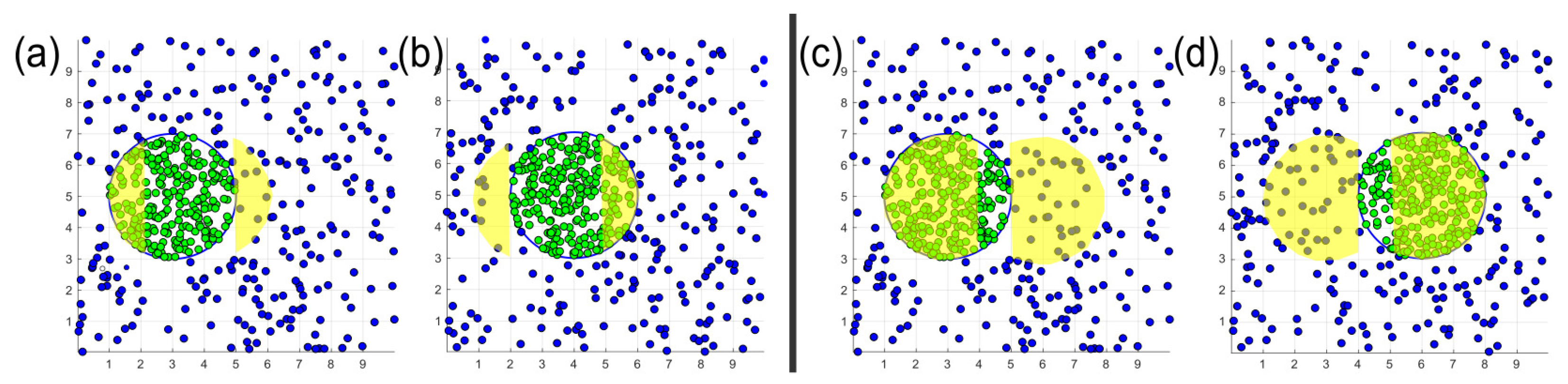
Figure 2.
The left side represents a low-severity concept drift: yellow areas in (a,b) indicate regions that should be forgotten and learned, respectively, after the drift. The right side represents a high-severity concept drift: yellow areas in (c,d) indicate regions that should be forgotten and learned, respectively, after the drift.
Figure 3.
Example of the influence zone descriptor: (a) the decision boundary is defined by and . (b) After the drift, the decision boundary is shifted to and . (c) The displacement of the decision boundary results in a region of conflict between concepts delimited by .
Figure 4.
(a) An abrupt drift occurs when the current concept , which ends at , is replaced by a new concept . (b) An incremental gradual drift is a slow transformation of the current concept into the new concept, with a transition period of length n, during which instances of both concepts no longer coexist, producing n intermediary concepts. (c) A probability gradual drift is a slow transformation between concepts where instances of both concepts coexist; the probability of the current concept gradually decreases to 0, while the probability of the new concept concurrently increases to 1.
Figure 5.
(a) Two examples of drift with non-periodic frequency. The first, between the yellow and green concepts, has frequency . The second drift has of frequency (green and pink concepts), where . (b) Recurrent cyclical drift, where and represent the frequencies of concepts 1 and 2, respectively. (c) Recurrent acyclic drift, where and represent the frequencies of concepts 1 and 2, respectively.
Figure 6.
(a) Relationship between severity and frequency with dissimilarity between concepts in time tuples (; ) and (; ). (b) Four states result from the relationship between these descriptors.
Figure 7.
Experiment overview.
Figure 8.
Performance metrics of drift detectors in scenarios by context. The horizontal axis of each heatmap represents the scenarios. The vertical axis represents the datasets Circle (C), Line (L), Hyperplane (H), SineV (SV), and SineH (SH).
Figure 9.
Values of the medians of prequential error across all datasets.
Figure 10.
Variation in prequential error median on all scenarios investigated by varying the value of each descriptor considering supervised detectors. Speed: (A) Abrupt; (G) Gradual. Severity: (H) High; (L) Low. Recurrence: (R) Recurrent; (NR) Not Recurrent. Frequency: (PH) Periodical High; (PM) Periodical Middle; (PL) Periodical Low; (NP) Not Periodical.
Figure 11.
Variation in prequential error median on scenarios investigated by varying the value of each descriptor considering the semi-supervised and unsupervised detectors. Speed: (A) Abrupt; (G) Gradual. Severity: (H) High; (L) Low. Recurrence: (R) Recurrent; (NR) Not Recurrent. Frequency: (PH) Periodical High; (PM) Periodical Middle; (PL) Periodical Low; (NP) Not Periodical.
Table 1.
A comparison of related work in terms of evaluated descriptors.
| Work | Descriptors | Group |
|---|
| SP | SV | IZ | FQ | RR | PD |
| Guo et al. (2022) [4] | • | | | | • | | 1 |
| Dasu et al. (2006) [28] | | | • | | | |
| Hinder and Hammer (2021) [30] | | | • | | | |
| Dong et al. (2017) [33] | | | • | | | |
| Dong et al. (2021) [34] | | | • | | | |
| Agrahari and Singh (2022) [38] | | | | • | | |
| Mattos et al. (2021) [39] | | • | | | | |
| Hinder et al. (2020) [2] | | • | | | | | 2 |
| Aguiar and Cano (2024) [35] | | | • | | | |
| Hammer et al. (2024) [36] | | | • | | | |
| Wang et al. (2024) [40] | • | • | | | | |
| This work | • | • | | • | • | |
Table 2.
Summary of the relationships between descriptors that affect base classifier and detector performance.
| Group 1 Impact on the performance of the base classifier and the detector |
| Descriptor | Descriptor | Impact |
| Severity | Frequency |
| High | Low | High |
| High | High | High |
| Low | High | High |
| Low | Low | Low |
| Severity | Influence Zone | Impact |
| High | Global | High |
| High | Local | High 1/Low 2 |
| Low | Local | Low |
Table 3.
Summary of relationships between descriptors that affect the behavior of descriptors.
| Group 2 Impact on the behavior of descriptors |
| Descriptor | Descriptor |
| Frequency | Speed |
| ↑ (Increases) | ↑ (Increases) |
| ↓ (Decreases) | ↓ (Decreases) |
| Recurrence | Frequency |
| Yes | Majority 1 |
Table 4.
Summary of relationships between descriptors that affect the predictability of concept drift.
| Group 3 Impact on the predictability of concept drift |
| Descriptor | Pattern | Descriptor | Predictable |
| Speed | Yes | Predictability | Yes |
| Frequency | Yes | Predictability | Yes |
| Recurrence | Yes | Predictability | Yes |
Table 5.
Values of descriptors by scenarios.
| Scenario | Description 1 | #Drift | Speed | Frequency | Scenario | Description 1 | #Drift | Speed | Frequency |
|---|
| 1 | A-H-R-PH | 39 | 1 | 250 | 17 | G-H-R-PH | 39 | 250 | 250 |
| 2 | A-H-R-PM | 9 | 1 | 1000 | 18 | G-H-R-PM | 9 | 250 | 1000 |
| 3 | A-H-R-PL | 3 | 1 | 3000 | 19 | G-H-R-PL | 3 | 250 | 3000 |
| 4 | A-H-R-NP | 9 | 1 | Alt 2 | 20 | G-H-R-NP | 9 | 250 | Alt 2 |
| 5 | A-H-NR-PH | 39 | 1 | 250 | 21 | G-H-NR-PH | 39 | 250 | 250 |
| 6 | A-H-NR-PM | 9 | 1 | 1000 | 22 | G-H-NR-PM | 9 | 250 | 1000 |
| 7 | A-H-NR-PL | 3 | 1 | 3000 | 23 | G-H-NR-PL | 3 | 250 | 3000 |
| 8 | A-H-NR-NP | 9 | 1 | Alt 2 | 24 | G-H-NR-NP | 9 | 250 | Alt 2 |
| 9 | A-L-R-PH | 39 | 1 | 250 | 25 | G-L-R-PH | 39 | 250 | 250 |
| 10 | A-L-R-PM | 9 | 1 | 1000 | 26 | G-L-R-PM | 9 | 250 | 1000 |
| 11 | A-L-R-PL | 3 | 1 | 3000 | 27 | G-L-R-PL | 3 | 250 | 3000 |
| 12 | A-L-R-NP | 9 | 1 | Alt 2 | 28 | G-L-R-NP | 9 | 250 | Alt 2 |
| 13 | A-L-NR-PH | 39 | 1 | 250 | 29 | G-L-NR-PH | 39 | 250 | 250 |
| 14 | A-L-NR-PM | 9 | 1 | 1000 | 30 | G-L-NR-PM | 9 | 250 | 1000 |
| 15 | A-L-NR-PL | 3 | 1 | 3000 | 31 | G-L-NR-PL | 3 | 250 | 3000 |
| 16 | A-L-NR-NP | 9 | 1 | Alt 2 | 32 | G-L-NR-NP | 9 | 250 | Alt 2 |
Table 6.
Comparing descriptors in each context using statistical tests.
| Context | Speed | Severity | Recurrency | Frequency |
|---|
| A | G | p-Value | H | L | p-Value | R | NR | p-Value | PH | PM | PL | NP | p-Value |
|---|
| DDM | | 16.6 | | | 14.5 | <0.05 | | 16.0 | | 14.2 | | | | |
| EDDM | 16.2 | | | | 15.1 | | | 12.7 | <0.05 | | | 9.4 | | <0.05 |
| DDM-O | | 15.4 | | | 14.9 | <0.05 | 14.3 | | <0.05 | | | 9.2 | | <0.05 |
| EDDM-O | | 15.8 | | | 13.6 | <0.05 | | 14.5 | <0.05 | | 15.4 | | | |
| DDAL | | 14.5 | | | 12.2 | <0.05 | | 15.1 | | | | 10.2 | | <0.05 |
| STUDD | | 14.9 | | | 12.1 | <0.05 | | 13.8 | | | | 10.0 | | <0.05 |
| MD3-EGM | | 16.9 | | | 14.8 | <0.05 | | 15.9 | | 14.4 | | | | |
| DSDD | | 15.8 | | | 13.6 | <0.05 | | 14.5 | <0.05 | | 15.4 | | | |
| ND | | 14.7 | | | 12.0 | <0.05 | | 14.8 | | | | 10.0 | | <0.05 |
Table 7.
Values of descriptors for the best and the worst results.
| Results | | Speed | | Severity | | Recurrency | | Frequency |
|---|
| | A | G | | H | L | | R | NR | | PH | PM | PL | NP |
|---|
| Best | | | 8/9 | | | 9/9 | | | 8/9 | | | | 5/9 | |
| Worst | | 8/9 | | | 9/9 | | | 8/9 | | | 7/9 | | | |
| Disclaimer/Publisher’s Note: The statements, opinions and data contained in all publications are solely those of the individual author(s) and contributor(s) and not of MDPI and/or the editor(s). MDPI and/or the editor(s) disclaim responsibility for any injury to people or property resulting from any ideas, methods, instructions or products referred to in the content. |
© 2025 by the authors. Licensee MDPI, Basel, Switzerland. This article is an open access article distributed under the terms and conditions of the Creative Commons Attribution (CC BY) license (https://creativecommons.org/licenses/by/4.0/).


