Risk Mutualization in Central Clearing: An Answer to the Cross-Guarantee Phenomenon from the Financial Stability Viewpoint

Abstract

Central counterparties’ (CCPs) role is to take over the counterparty risk during trading. To fulfill its role, a CCP needs to operate a multi-level guarantee system that can absorb losses of clearing members’ defaults. Our main question is how the size of the guarantee system changes and how the cross-guarantee undertaking changes between clearing members and markets if the CCP merges the guarantee systems of different markets. This question is essential from a financial stability perspective since the size and the structure of the guarantee system will affect the loss-absorbing capacity of a CCP. We used Monte Carlo simulation to simulate a 30 year time-series for three different products, which gave us the basis for the value-at-risk-based margin calculation and the stress-test-based default fund calculation. Results show that merging the guarantee systems will always decrease the total value of the guarantees because the margin will decrease, which cannot be offset by the increase in the default fund size. We conclude that it is not optimal from the financial stability perspective to merge the guarantee systems. However, if the CCP wants to provide cheaper services, or if the clearing members are willing to cross-guarantee each other, merging is more suitable.

1. Introduction

Over the last decade, the financial markets’ regulatory changes have been aiming to increase the system’s resilience and seeking to reduce systemic risk to increase financial stability. Financial stability means that the system is able to facilitate and enhance economic processes, can manage risk, and moreover, can absorb losses (Schinasi 2004). The structural modifications introduced require that over-the-counter (OTC) derivatives should be cleared through central counterparties (Platt et al. 2017). Authorities have also put great attention into strengthening the global safeguards for central clearing to prevent failures and massive distress by adopting the CPMI-IOSCO Principles for Financial Market Infrastructures in 2012, dedicated Financial Stability Board guidance, and the European Market Infrastructure Regulation (EMIR) in 2012.

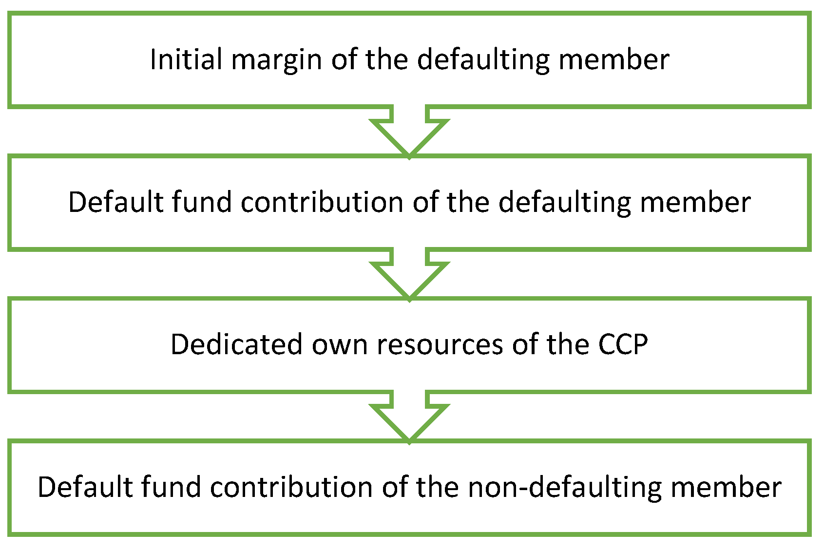
The clearing activity of CCPs means that they take over counterparty risk during trading by becoming the buyer/seller of every sell/buy trade. According to this, if one of the trading partners defaults, the CCP will guarantee for the non-defaulting members that the trade will be fulfilled. To ensure financial resources that are enough to cover the losses caused by the default of one or more clearing members, a default waterfall system is operated. The three typical resources of the waterfall system are the initial margin (IM) requirements, the skin-in-the-game (SITG), and the default fund (DF) contributions. The default waterfall system, required to be operated by all CCPs, assures these market infrastructures’ resilience and loss-absorbing ability to enhance financial stability in the economy. In Figure 1, the elements of this default waterfall system can be seen according to the requirements of Article 45 of the EMIR (2012) regulation, whose framework has been in force in the European Union since 2012. Our research is based on the EMIR, so we will not cover the requirements of other regulations related to CCPs’ risk management, e.g., the Dodd–Frank Act (2010). Braithwaite and Murphy (2016) explains how the default waterfall system is built up and details its origin.

The exhaustion of the above-listed resources is far from random. EMIR requires using the available balances in a preordered sequence. The first resources to be exhausted are the initial margin requirements. According to Figure 1, a CCP at first can only use the margin to cover losses of the defaulting member but not the resources of the non-defaulting members. Based on EMIR Article 41 (EMIR 2012) and chapter VI of the regulatory technical standards (RTS 2013), the level of margin requirements should be set to cover potential market losses in the clearing members’ positions in normal market conditions, based on the calculation of a statistical model. Procyclicality should also be taken into consideration (e.g., Glasserman and Wu 2017). The different procyclicality handling methods are being analyzed by Berlinger et al. (2018), while procyclicality was analyzed by King et al. (2020) from a liquidity point of view. The discrepancies related to margin calculation in the regulatory framework are interpreted by Murphy et al. (2014, 2016) and Szanyi et al. (2018).

Available margin resources are then followed by the default fund contribution sources based on Article 45 (EMIR 2012), which is the mutualized layer of resources provided by clearing members (Murphy 2017). This means that not only the defaulting member’s contribution can be applied to cover losses by a CCP but the non-defaulting ones’ as well. Nevertheless, in the second layer, only the defaulting members’ default fund contribution can be used. Our paper defines the default fund on the max(1;2+3) concept. This means that the default fund should, at least, enable the CCP to stand, under extreme but plausible market conditions based on Article 42 (EMIR 2012), for the clearing member’s default with the greatest exposure or the sum of the second and third largest exposures of clearing members. Exposure means the losses that the value of the initial margin cannot cover. As a result, the smaller the initial margin is, the larger the default fund will be ceteris paribus (Murphy 2013; Nahai-Williamson et al. 2013; Cumming and Noss 2013). CCPs usually define the extreme but plausible market conditions in a stress test framework by creating historical and hypothetical stress scenarios. The scenarios should include the most volatile periods that the markets have experienced in the last thirty years for which the CCP provides its services (historical scenarios) and a range of potential future scenarios (hypothetical scenarios), taking into account the correlation between the different traded financial assets based on Article 30 (RTS 2013). The default fund contributions are proportional to the exposures of each clearing member (EMIR Article 42, RTS Chapter VII).

Risk management tasks do not stop here; the CCP itself also contributes some part of its own capital to the default waterfall system, which should be 25% of its minimum capital (RTS 2013, Article 35). This layer is called the skin-in-the-game. If all the defaulting members’ resources are exhausted, the CCP’s SITG will be consumed (McPartland and Lewis 2017). If this layer is not enough to cover the losses, the last layer will be applied, namely, the non-defaulting members’ default fund contribution. This means that the cross-guarantee between clearing members appears in this layer. Baker (2021) and Huang and Takáts (2020) highlight the risks associated with the skin-in-the-game, including those that can shape incentives. Overall, CCPs and market participants should work together to ensure the most suitable practices are implied (Friesz 2020).

In practice, CCPs may decide to use an additional final layer, namely, a specific portion of the CCP’s own capital, as a second skin-in-the-game, additional own resources (EACH 2021), but this layer is voluntary by the CCPs. If the default waterfall is still insufficient, recovery and resolution regimes are put into force (Cont 2015).

Principle 7 CPSS-IOSCO and the EMIR regulation introduce the Cover 2 concept as well, meaning that CCPs should have sufficient liquidity—should have enough guarantees within the whole default waterfall—to cover the simultaneous default of the two clearing members—and their affiliates—which would generate the most significant exposures against the CCP (Parkinson 2014). Murphy and Nahai-Williamson (2014) state that the Cover 2 standard is prudent, but in practice, it would be worth seeing the distribution of all of the losses to ensure that the guarantee system of the CCPs is robust enough in every case. Poce et al. (2018) support this and found that in the case of notable systemic events, the default fund is not adequate to cover losses in the Cover 2 concept, only in the case of very conservative CCPs. Capponi et al. (2018, 2020) have built up a method that could be used to define the optimal cover rule for defining the default fund. At the same time, Paddrik and Young (2017) show that two members’ simultaneous failure could cause network contagion and lead to insufficient funds at the CCP. Campbell and Ivanov (2016) argue that the losses could be more substantial if large CCP members’ exposures are positively correlated than if they are independent. Tywoniuk (2020) shows concern regarding potential contagion due to their high level of interconnectedness. Ghamami and Glasserman (2017) have found that lower default fund requirements reduce the cost of clearing but make CCPs less resilient. Barker et al. (2016) have analyzed the distribution of losses to default fund contributions and contingent liquidity requirements for each clearing member, identifying wrong-way risks among defaulting parties. Their main conclusion suggests that liquidity is the most important for members assessing the risks and costs.

Finally, Berndsen (2020) summarizes the most important research topics on CCPs, grouping them by the main fields they cover, namely, the clearing activity, the optimal number of CCPs, the default waterfall’s size, the exhaustion of the default waterfall, and skin-in-the-game related researches. Also Menkveld and Vuillemey (2021) give a comprehensive summary of research on CCPs.

In our paper, we contribute to the existing literature as we analyze the effect of merging different market guarantee systems from the viewpoint of having a common default fund for different markets or having them separately for spot and derivative trades on the securities market. To our best knowledge, the literature lacks analysis on how merging different markets’ default waterfall affects the structure and the size of the initial margin and default fund contributions of the clearing members. It is vital to notice that if the default funds are common in this paper, then the whole default waterfall will be handled as common. Our paper’s primary focus will be to show how the margin and default fund size will change and how their value will change compared to each other. We analyze it on the whole guarantee system level and the individual clearing member level since we want to show the effect of risk mutualization. This means that we intend to analyze whether the risk-averse clearing members will take over risk from risk-seeking clearing members on the jointly cleared markets since the initial margin and default fund will increase for them ceteris paribus compared to the separated markets. We carried out our analysis on 30 year simulated data by applying a Monte Carlo simulation. In practice, it is common to have separated default funds (e.g., KELER CCP 2021) because separated default waterfalls do not mutualize risk. For example, it was seen in 2012 in the case of LCH.Clearnet, which split its default fund based on this reason (Jaidev 2012).

2. Related Literature of Stress Tests

The size of the guarantees the clearing members have to pay is an essential question from their viewpoint not only on the individual clearing members’ but also from the CCP’s, since the lower the value of the margin and default fund, the lower the cost of trading, and liquidity risk can be decreased as well. In this paper, under liquidity risk, we mean the risk of not having enough resources by the clearing members to finance the margin and the default fund contribution requirements. From a CCP’s point of view, the lower value of the guarantee system elements also means that it can have a competitive advantage in giving clearing services on the market. However, we should also keep in mind that the lower the guarantees’ value, the higher risk is being run by the CCPs, since the guarantee system is not as vulnerable. From a systemic risk and a financial stability perspective, it is a crucial question since CCPs are systematically important financial institutions in the financial markets. So what may be optimal for the individual participants—whether they are the clearing members or the CCPs themselves—is not necessarily good from a financial stability perspective. Due to the interconnectedness of CCPs, many have criticized the risk CCPs carry as “being too big to fail” due to their continually growing importance (Chamorro-Courtland 2011; Cont 2015; Duffie et al. 2015; Berlinger et al. 2018). Markose et al. (2012) mentions the concept of “too interconnected to fail”, fearing the domino effect in case of distress. This systematic risk aspect has been analyzed by many from different viewpoints; for example, Biais et al. (2012) highlight moral hazard and risk monitoring (Biais et al. 2016) issues, while Lopez and Saeidinezhad (2017) analyze CCPs resilience, not in isolation, but potential spillovers on the rest of the financial system. They point out that regulators should implement further guidelines to assure financial stability. The supervisory stress tests, performed in 2019 in the EU and the United States, have started focusing more and more on the institutions’ linkages (ESMA 2019; US CFTC 2016). McLaughlin and Berndsen (2021) recalled the main historical events of CCPs facing severe stress events. They conclude that legal discrepancies were acknowledged since the subprime crisis, and steps for improvements were taken. Faruqui et al. (2018) analyze the CCP-bank nexus, focusing on the two-way interactions between them. Along the balance sheet interlinkages and the structure of the CCP default waterfall, they show the nexus between them and highlight that the levels of stress change these interactions, and the endogenous build-up of risk connections can be harmful. King et al. (2020) analyze the events from September 2018 on the Swedish market, also discussing the benefits of CCPs.

We focused on the default funds’ design, and we calculated the size of the default funds based on the stress test methodology, using a simulation of 30 years. According to EMIR (2012, Article 49), stress tests should be used to test and measure the risk management models of the CCPs in extreme but plausible market conditions. However, the regulatory framework may be vague in some aspects, so the methodologies and the most proper calibration of models gained immense attention. Novick et al. (2014) advise in their research that it would be necessary to mandate a standard stress test methodology for all CCPs. On the contrary, in practice, a wide variety of models have been developed to determine the adequate stress testing method. For example, the design of stress scenarios was analyzed by Canabarro (2013), while Poce et al. (2018) introduced a network-based stress test for CCPs. Bo et al. (2021) showed the premature failure of a CCP during a market shock if it loses its superiority to bilateral clearing. Paddrik and Young (2021) indicated that on CDS markets, conventional stress testing approaches may underestimate the potential threats of a CCP.

Stress tests aim to measure the resilience of an institution to ensure the availability of adequate resources. Furthermore, interconnectedness and systemic risks are also quantified. Therefore, the institutions themselves mark a set of parameters and shock the systems with independent events. The results define risk factor changes and then outline the extent of losses suffered in different scenarios. Madar (2010) defines stress tests as the techniques that measure the effects of rarely occurring events that are not measurable by the usual toolkit on financial institutions (Madar 2010). The exact course of preparing stress tests is described in detail by Hilbers and Jones (2004).

The types of stress tests may differ based on grouping principles. The BCBS (2009) groups test by the sensitivity analysis complexity or the built scenario applied. While Cihák (2007) argues the institution’s scope versus the whole financial system, the Central Bank of Hungary (2019) advises bottom-up or top-down analysis. Hull (2015) defines the historical and hypothetical sources of scenarios, and Banai et al. (2013) run stress tests built upon the number of risks taken into consideration. The number of assets tested and the applied time horizon of the stress test may also be criteria.

In recent years, regulators set out a stress test methodology framework, called the “EU wide stress test”, performed by the European Securities Market Authority (ESMA) at least annually. The latest stress tests were published in July 2020 (ESMA 2020). With local authorities, ESMA applies common methodologies for assessing the effect of different stress scenarios and has identified the shortcomings in the institutions’ resilience. During the tests, credit, liquidity, concentration risk, and reverse credit stress are analyzed.

3. Model

Our main question is how the default waterfall’s size and structure changes regarding the initial margin and default fund size if we clear two markets separately or jointly and how it affects risk mitigation. We chose two markets: the spot market for securities and the derivative market for these securities. It was important to select two markets that have a connection with each other because we wanted to show how the risk mitigation of the hedged positions between the spot and derivative assets changed the riskiness of the positions of the clearing members, and as a consequence, the guarantees the clearing members have to pay after their positions. We built a theoretical model using a Monte Carlo simulation (MCS). During our analysis, we did not simulate or include the value of the SITG. Our model had one CCP, four different clearing members, and three different financial assets: a stock, a bond, and a currency. The stock could be traded on the options, futures, and spot markets, while the bond could be traded only on the futures and spot markets, and the currency could be traded only on the options and futures markets. For the MCS, we had to have an assumption for the financial assets’ price evolution since we needed a time-series for initial margin calculation and for estimating the default fund. We chose the arithmetic Brownian motion (ABM) to simulate the daily logreturns of the stock and the currency, while we chose the Vasicek model (Vasicek 1977) to simulate the instantaneous rate in the case of the bond. Based on this, Equation (1) shows the ABM we use for the stock and the currency:

$$dY=\alpha ·dt+\sigma ·\sqrt{dt}·N\left(0,1\right)$$

(1)

where “dY” is the change in the logreturn during “dt” period, “α” is the expected value of the logreturn, “σ” is the standard deviation for the logreturn, and “N(0,1)” is a standard normal random variable. The price is determined by Equation (2), where “t” stands for time, and “S” stands for the asset’s price:

$$S_t=S_0·e^{Y_t}$$

(2)

In our simulation, the stress test had a central role. We simulated 30 years—since this is the look-back period for defining historical scenarios within the EMIR regulation—for both financial assets. To simulate the price of the stock and the currency, we set the value of the parameters needed to run the simulation. Moreover, to use “realistic” values in the simulation, which represent the European stock market and currency market, we estimated the expected value of the logreturn (α) and standard deviation (σ)—between 12 January 1991 and 11 January 2021—of the DAX index, and—between 1 December 2003 and 11 January 2021—for the EUR/USD (Finance.yahoo.com 2021a, 2021b). Unfortunately, the time-series for the EUR/USD was not available for 30 years since the EUR has not existed for 30 years. The first day’s price in the simulation was the price of DAX on 12 January 1991 and the price of EUR/USD on 1 December 2003. The applied parameters can be seen in

Table 1. The parameters of the price simulation in the case of the stock and the currency.

Parameter	Stock	Currency
α	7.71%	0.09%
σ	22.37%	11.85%
S0	1345.26	1.1965
dt	1 day	1 day

.

In the case of the bond, we applied the Vasicek model (Vasicek 1977) determined in Equation (3):

$$d{y}_t=a·\left(b-y_t\right)dt+\sigma \ast \sqrt{dt}·N\left(0,1\right)$$

(3)

where “dy” is the change in the instantaneous interest rate “y”; “a” is the speed of reversion to “b”, which is the long term mean level; “σ” is the instantaneous volatility of “y”. Based on the model, the bond price (“P”) is the following according to Equations (4)–(6), where “T” is the maturity of the bond (Mamon 2004).

$$A\left(t,T\right)=\frac{1-e^{-a\left(T-t\right)}}{a}$$

(4)

$$D\left(t,T\right)=\left(b-\frac{{\sigma }^2}{2a^2}\right)\left[A\left(t,T\right)-\left(T-t\right)\right]-\frac{{\sigma }^{2}A{\left(t,T\right)}^2}{4a}$$

(5)

$$P\left(t,T,y_t\right)=exp\left(-A\left(t,T\right)y_t+D\left(t,T\right)\right)$$

(6)

The applied parameters for the bond price simulation can be seen in

Table 2. The parameters of the price simulation in case of the bonds.

Parameters for the Price Simulation
Vasicek	Bond
a	5
σ	2.49%
b	12.20%
y0	2.69%
T	5
dt	1 day
Face value	100

. The parameter estimation basis is the monthly time-series data of the term structure of interest rates on listed federal securities with a residual maturity of 0.5 years between the time period of January 1991 and December 2020, also for 30 years for the stock and the currency.

In addition to the price evolution for the financial assets, we also assumed a correlation between the three financial assets’ returns. They did not evolve independently from each other. The correlation was taken into account through the N(0,1) standard normally distributed random number in all three processes. We applied the Cholesky decomposition, which means that the relation between the random variables is the following, based on Equations (7)–(9) (Medvegyev and Száz 2010), where “$ϵ$” will be a random number used in case of the three assets, and “ρ” is the correlation coefficient.

$${ϵ}_{stock}=N{\left(0,1\right)}_{Stock}$$

(7)

$${ϵ}_{currency}=\rho ·N{\left(0,1\right)}_{Stock}+\sqrt{1-{\rho }^2}·N{\left(0,1\right)}_{Currency}$$

(8)

$${ϵ}_{bond}=\rho ·N{\left(0,1\right)}_{Stock}+\frac{\rho -{\rho }^2}{\sqrt{1+{\rho }^2}}·N{\left(0,1\right)}_{Currency}+\sqrt{1-{\rho }^2-\frac{{\left(\rho -{\rho }^2\right)}^2}{1-{\rho }^2}}·N{\left(0,1\right)}_{bond}$$

(9)

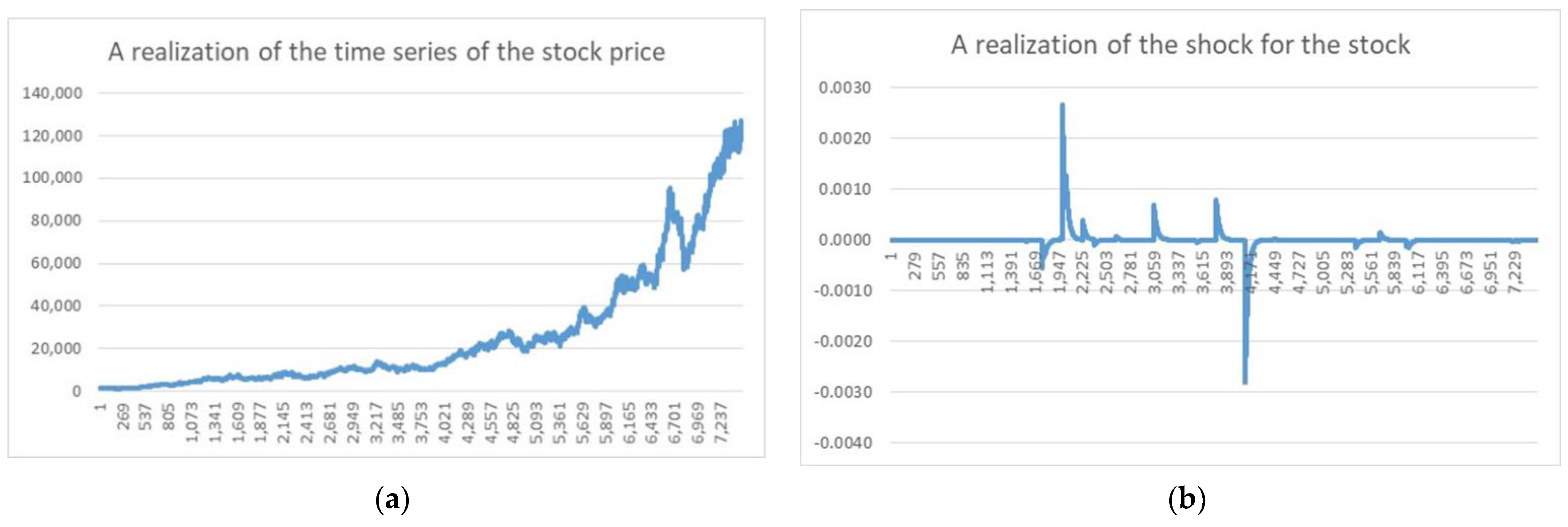
The correlation between the assets is 0.2 in normal market conditions. However, in our price simulation, it was not enough to capture the normal market conditions since we needed stress/shocks in the simulated time-series as well. As we stated before, the initial margin stands for covering possible losses in normal market conditions, while the default fund should cover the losses in extreme but plausible market conditions, which we estimate with stressed market events. As a result, we modified the simulation of the logreturns of the three assets by simulating stresses in the time-series of assets’ returns as well, so the ABM and Vasicek were not enough for us as we presented before. The stress/shock occurrence was modeled with a Poisson process, while the extent of the shock was modeled with a lognormal distribution. The correlation at the time of the shock—in the case of any of the assets—was increased to 0.95, and it decreased by 0.95 every day. The applied parameters for the model are the following according to

Table 3. The parameters of the shock simulation.

Shock Parameter Affecting the Value of the Shock
	Stock	Currency	Bond
μ	−10.00	−10.00	−10.00
σ	2.25	2.25	2.25
decrease of shock	0.97	0.97	0.97
Shock Parameters Affecting the Date of the Shock
λ	0.005	0.0045	0.004

, while a realization of the stock price and one realization of the shock can be seen in Figure 2.

Four clearing members (CM) were present on the market, with different positions according to

Table 4. Number of positions of clearing members.

Position of Clearing Members	Clearing Member 1			Clearing Member 2			Clearing Member 3			Clearing Member 4
	Stock	Bond	Currency	Stock	Bond	Currency	Stock	Bond	Currency	Stock	Bond	Currency
Long Put	3		5	2
Short Put							5		5
Long Call	3		5
Short Call							3		5
Long Futures		5			5	5
Short Futures			5					10
Long Underlying				2			3			6	5
Short Underlying	8				5					3
Name of position	Long straddle + spot	Futures	Long straddle + futures	Protective put	Futures + spot	Futures	Covered call + short straddle + spot	Futures	Short straddle	Spot	Spot	---

. The positions of the clearing members were built in order to be able to analyze how the merged and separated default funds affected the margin and default fund contributions of the markets. CM4 had positions only on the spot market, while the other clearing members had risky positions, such as short straddles, and also positions that handled risk, such as protective put or covered call positions. This is important because if the markets are cleared separately, this risk hedging cannot be used by the clearing members regarding initial margin and default fund payment, while on the merged market, they can hedge the risk. CM3 takes the riskiest position since it has large unhedged short futures positions and also unhedged short straddles as well.

In the following, we show how we estimate the initial margin and the default funds from the simulated times series data and the clearing members’ positions. The margin of the underlying assets (stock, bond, currency) is calculated by Béli and Váradi’s (2016) method. This model is based on the delta-normal value-at-risk (VaR) calculation (Jorion 2007) using different standard deviations to quantify the VaR value. Namely, we calculated the equally weighted standard deviation (${\sigma }^{equal})$and the exponentially weighted moving average (EWMA) standard deviation (${\sigma }^{EWMA})$ of the time-series of the simulated logreturns (from Equation (1)) in the case of the stock and the currency, while in the case of the bond, the standard deviations should be calculated for the change of the simulated returns from the Vasicek model. Always that type of standard deviation is applied, which has a lower value, according to Equations (10) and (11),

$$Va{R}_t^y=min\left({\sigma }^{equal}·N^{-1}\left(99\%\right);{\sigma }^{EWMA}·N^{-1}\left(99\%\right)\right)$$

(10)

$$Va{R}_{t, bond}^y=D^{\ast }·min\left({\sigma }^{equal}\left(\Delta y_t\right)·N^{-1}\left(99\%\right);{\sigma }^{EWMA}\left(\Delta y_t\right)·N^{-1}\left(99\%\right)\right)$$

(11)

where N⁻¹(99%) is the inverse of the normal distribution’s cumulative distribution function at the 99% probability, D* is the modified duration of the bond, $Va{R}_t^y$ is the value-at-risk at day t for the logreturn (y) in case of the stock and the currency, while $Va{R}_{t,bond}^y$ is the value-at-risk for the bond’s logreturn. The value-at-risk expressed for the price instead of the logreturn is based on Equations (12) and (13), where S is coming from the ABM (Equations (1) and (2)), while P is coming from the Vasicek model (Equations (3)–(6)), and T is the liquidaton period, which is set to 2 days, based on the regulation (EMIR 2012; RTS 2013),

$$Va{R}_t^{price}=-S_t+S_t·e^{\sqrt{T}·Va{R}_t^{yield}}$$

(12)

$$Va{R}_{t,bond}^{price}=abs\left(P_t·Va{R}_{t, bond}^y\right)$$

(13)

Additionally, a 25% procyclicality buffer was used. It was exhausted and built back based on the two standard deviations, and it worked the same way for all of the three products, so we will not highlight the bond separately as in the case of Equations (10)–(13). If the EWMA standard deviation is greater, then the buffer is exhausted gradually. If the equally weighted standard deviation is greater, it is gradually built back, according to Equations (14)–(16), where π stands for the procyclicality buffer

$$PROmargi{n}_t=Va{R}_t^{price}·\left(1+\pi \right)$$

(14)

$$margi{n}_t^{\pi exhaustion}=\max \left(margi{n}_{t-1};Va{R}_t^{price}\right)$$

(15)

$$margi{n}_t^{\pi built back}=\min \left(margi{n}_t^{\pi exhaustion};PROmargi{n}_t\right)$$

(16)

Finally, the margin at time t is defined by Equations (17)–(21) for all three products by calculating a so-called margin band with a minimum and maximum margin value in Equations (17) and (18).

$$\begin{array}{c}MINmargi{n}_t=if\left({\sigma }^{EWMA}·\max \left(\frac{margi{n}_{t-1}}{Va{R}_t^{price}};1\right)>{\sigma }^{equal}\right);\\ margi{n}_t^{\pi built back};PROmargi{n}_t \end{array}$$

(17)

$$MAXmargi{n}_t=MINmargi{n}_t·\left(1+band\right)$$

(18)

If the calculated margin in Equations (10)–(16) does not reach this minimum or maximum value, the margin requirement will not change, according to Equations (19)–(21). The main goal of this calculation is to stabilize the value of the margin, not to have to change it on a daily basis, which is essential in practice from the clearing members’ liquidity management point of view.

$$margi{n}_t=if\left(margi{n}_{t-1}>MAXmargi{n}_t;MAXmargi{n}_t\right)$$

(19)

$$margi{n}_t=if\left(margi{n}_{t-1}<MINmargi{n}_t;MINmargi{n}_t\right)$$

(20)

$$margi{n}_t=if\left(MAXmargi{n}_t>margi{n}_{t-1}>MINmargi{n}_t;margi{n}_{t-1}\right)$$

(21)

After defining the margin on the individual asset level, we quantified the portfolio level margin. We carried it out by using the SPAN (standard portfolio analysis of risk) method by applying some simplification. The SPAN is a complex method, according to Figure 3 (CME Group 2019).

For simplicity, we assumed that there was only a risk array and short option minimum (SOM), which would be 10% of the underlying asset’s margin, except in the case of the bond; since there are no options, SOM is not needed either. The risk array contains scenarios for the portfolio, according to

Table 5. SPAN scenario parameters.

Scenario	The Change in Spot Price Will Be Multiplied by This Amount	The Change in Standard Deviation Will Be Multiplied by This Amount
1	0.00	1
2	0.00	−1
3	0.33	1
4	0.33	−1
5	−0.33	1
6	−0.33	−1
7	0.67	1
8	0.67	−1
9	−0.67	1
10	−0.67	−1
11	1.00	1
12	1.00	−1
13	−1.00	1
14	−1.00	−1
15	2.00	0
16	−2.00	0

. This means that the positions are revalued with the new underlying asset prices and new standard deviations. The scenario that gives the most significant loss is considered the margin (the Margin_CMt in Equation (22)) of a particular CM portfolio. One unit of change in the spot price is the value of the asset’s actual margin calculated in Equations (10)–(21), while one unit of change in the standard deviation is 90% of the actual daily standard deviation.

During portfolio-based margining, we determined the price of the options with the Black–Sholes model (Black and Scholes 1973). We assumed the following: the options are ATM options, with a maturity of one year; the standard deviation is the actual daily standard deviation that is used in the margin model; the one-year risk-free return is calculated with the Vasicek model; in the case of the currency option, the counter currency’s risk-free return is 0%. The futures positions have the same parameters as the options.

We simulated the margins on a portfolio level in two different ways, once when the margin and default fund were calculated for the spot and derivative markets as merged markets and once when they were separated. This is important because during the portfolio margining with the SPAN method in the merged case, the spot position could be hedged with the derivative position, hence, the risk is lower; therefore, the margin should be lower for the portfolio, while in the separated case, one portfolio is for the spot positions, and another portfolio is for the derivative positions, hence, the risk should be higher, and the margin should be higher as well. In our analysis, we aim to show this phenomenon, and also we want to show how it affects the value of the default fund, and as a final effect, how the size of the guarantees will change.

To calculate the default fund, we needed to run the stress test based on the EMIR (2012) regulation and Hull (2015). We estimated historical and hypothetical scenarios as well. Altogether, we had eight stress scenarios: six historical and two hypothetical in our stress test. In every scenario, we had a stress parameter for all three financial assets, one for the stock, one for the currency, and one for the bond. We used the same stress scenarios on the spot and derivative markets. The focus of our stress test was to see if we stress the current market price—which is the last simulated price in our price simulation with ABM and Vasicek, so the 7500th day—with every stress scenarios’ stress parameters, would the margin be enough to cover the potential losses in case the CM defaulted. According to EMIR, the value of the default fund is the scenario that has the highest loss of the max(1;2+3) exposures. We appled the following rule to define the historical scenarios: we took the simulated 30 year time-series and searched for the day where the stock had the lowest return. On this same day, we took the return of the bond and the currency as well. This was one scenario, and we named this “min stock.” The other five historical scenarios were based on the same method; summarized in the following, the six historical scenarios can be seen:

• Historical 1—Min stock: lowest stock return during the 7500 days and taking the currency returns and the bond yield change on the same day.
• Historical 2—Max stock: highest stock return during the 7500 days and taking the currency returns and the bond yield change on the same day.
• Historical 3—Min bond: lowest yield change during the 7500 days and taking the stock and currency returns the same day.
• Historical 4—Max bond: highest yield change during the 7500 days and taking the stock and currency returns the same day.
• Historical 5—Min currency: lowest currency return during the 7500 days and taking the stock returns and bond yield change the same day.
• Historical 6—Max currency: highest currency return during the 7500 days and taking the stock returns and bond yield change the same day.

In hypothetical scenarios, we must consider the correlation between the different risk factors and risk parameters. To fulfill the regulator’s requirements, we chose the stress parameters the European Systemic Risk Board (ESRB) put together during the EU-wide stress test for the central counterparties in 2019. The test’s time horizon was five days, but we ran our test only on a daily time horizon, so we converted the given parameters to daily ones. For the DAX index, −14% was given by the ESRB, so on a daily basis, it became −2.80%; the shortest government bond stress parameter belonged to the 1-year maturity bond, which was −36 basis points, so we applied −7.2 basis points. For the EUR/USD, the USD/EUR parameter was set at −5.8%, which means that the EUR/USD parameter was 6.16%, and on a daily basis it was 1.23% (ESRB 2019). We had two hypothetical scenarios, one with the parameters explained and another with the opposite of these numbers. An example of the eight stress scenarios based on our price simulation can be seen in

Table 6. An example of the stress scenarios.

	Historical Scenarios						Hypothetical Scenarios
Parameters	Min Stock	Max Stock	Min Currency	Max Currency	Min Bond	Max Bond	First	Second
Stock	−5.28%	4.71%	−0.48%	−1.59%	−1.59%	0.08%	−2.80%	2.80%
Bond	0.00%	0.00%	0.00%	0.00%	0.03%	−0.02%	−0.07%	0.07%
Currency	−1.26%	0.13%	−2.69%	2.90%	0.92%	−0.29%	1.23%	−1.23%
Number of day in the simulation	6839	179	3380	915	5897	5576

.

Overall, we define the largest and the sum of the second and third largest exposure (loss not covered by the initial margin) in every historical and hypothetical scenario. That scenario will “win” that has the largest exposure, so the one that had the largest max(1;2+3) value. Moreover, this value will be the value of the default fund (DF).

As a final step, this default fund (DF) is split up between the clearing members according to their ratio of margin payment within the total margin value on the market, according to Equation (22),

$${\mathrm{DF}}_{\mathrm{CM}1}=\frac{{\mathrm{Margin}}_{\mathrm{CM}1}}{{{\displaystyle \sum }}_{t=1}^4{\mathrm{Margin}}_{\mathrm{CMt}}}$$

(22)

4. Results

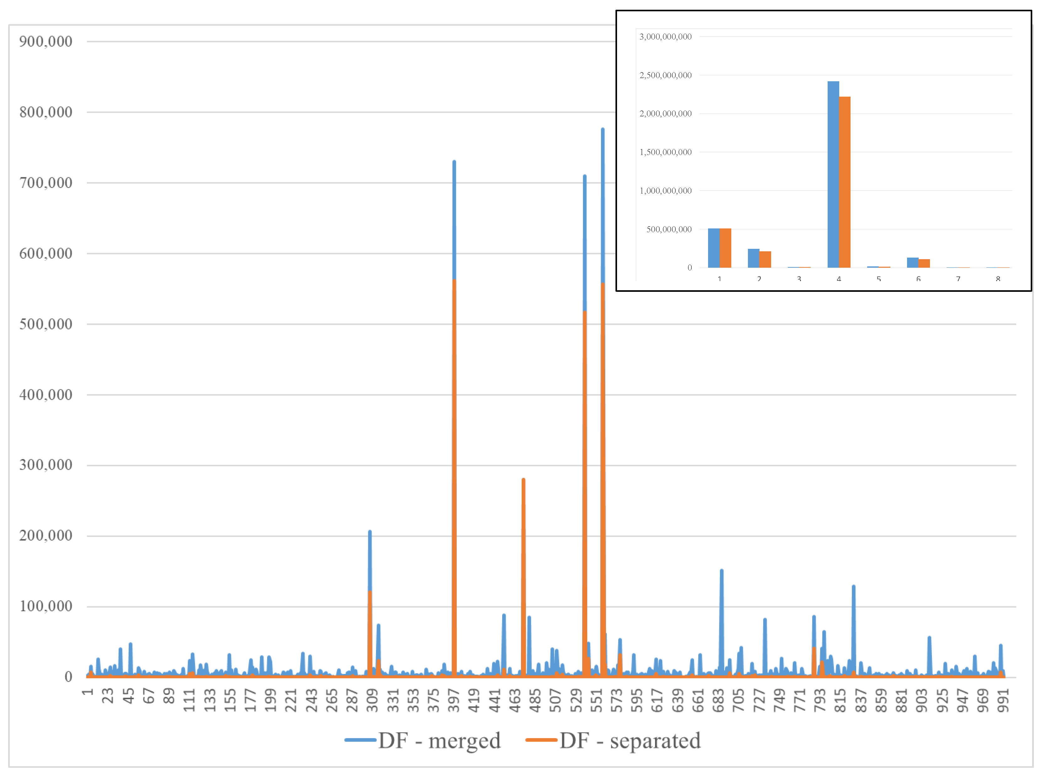
We ran the simulation 1000 times within the model we introduced in the previous chapter. Figure 4 shows the default funds’ values in the cases of merged and separated markets for 1000 realizations. In the separated DF-s, the value shown in Figure 4 is the sum of the DF of the spot and the derivative market. We cleaned our database of eight outlier values in order to represent the results since, in these outlier cases, the size of the default fund was so high that one graph could not contain all of them at once; the outliers can be seen in the right upper corner of Figure 4.

A striking difference can be seen between the markets regarding the value of the default fund (DF), namely, that the DF’s value was always higher in the merged market, which means that in the merged case, the cross-guarantee taken between the CMs became larger. Moreover, in the separated market, the DF value was 0 in 649 cases, while in the merged case, only one out of 1000. This is a vast difference, which is essential from a loss absorption point of view since zero DF value means that the value of the initial margin is enough to cover the losses both on the derivative and on the spot market as well in the separated structure, while in the case of the merged market, this could nearly never happen.

In the cleared dataset, the minimum DF value was zero in both market structures. While the separated DF had its maximum at 561,914, the merged DF was much higher: 776,197. The difference between the average DF value was more significant since the merged DF values’ average was more than three times as large, 7618, while in the separated, it was only 2419.

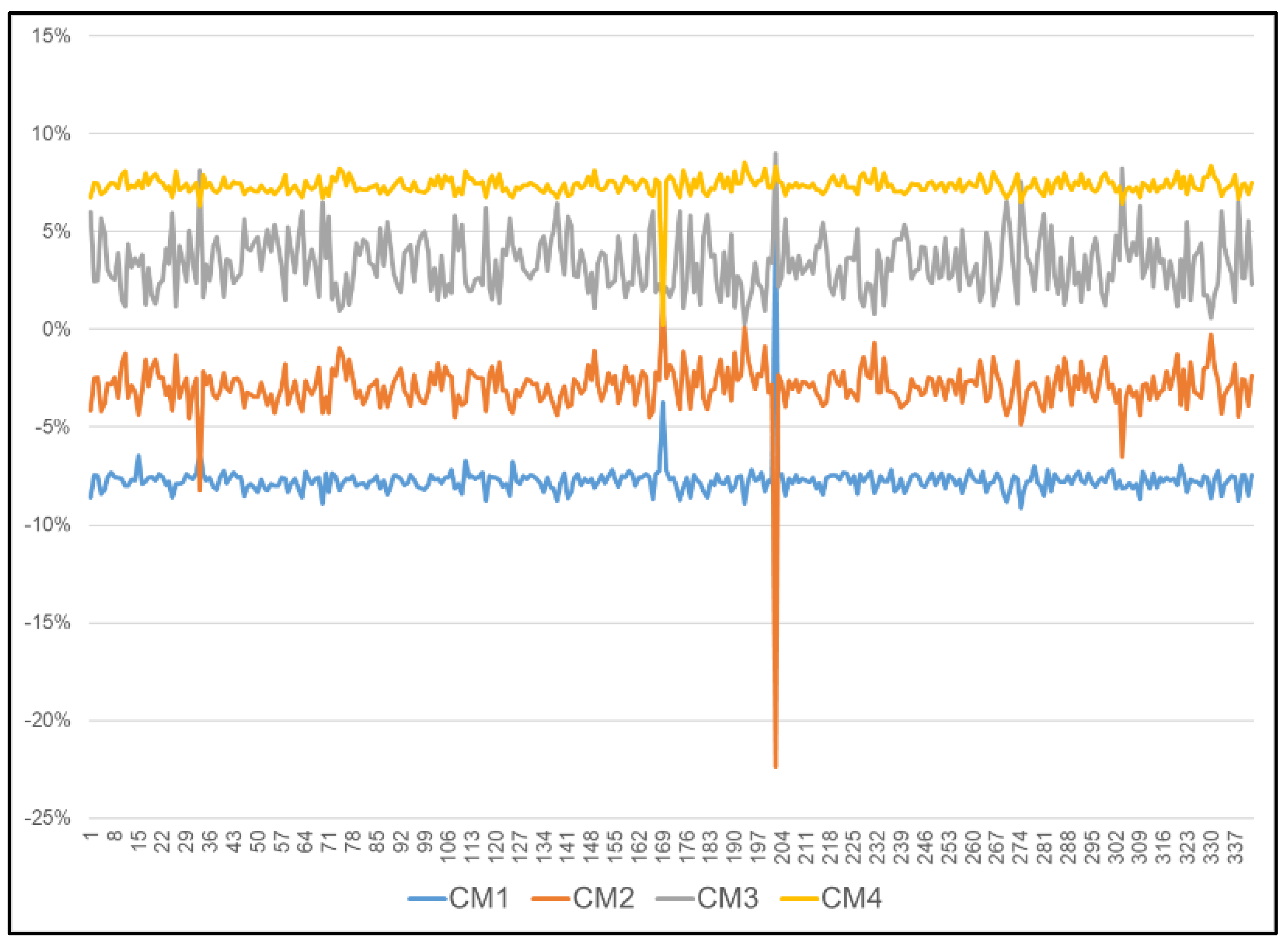
One of our goals was to examine how the contribution to the default fund changed per each clearing member in the two different structures, since we wanted to analyze how risk mutualization changes. To show this, we looked at how the default fund contribution—not in absolute terms, but the percentage of the total value of the DF—changed for each clearing member in the two cases. The result can be seen in Figure 5 for those cases when the DF was not 0 in the separated case. Figure 5 shows the difference between each CMs’ DF contribution within the merged and separated market. If the value is positive, the CM has a larger share in the DF in the merged case than in the separated, while if it is negative, the CM’s share was smaller.

The results show the DF contribution for CM3 and CM4 has always increased, while CM1 and CM2 consistently decreased, except one occasion out of the 1000 for CM1. CM3 only has net long positions in the stock and the bond, so it did not have any derivative positions. Merging the markets increases its share in the mutualized risk, so it has to face larger cross-guarantee commitments because of the high risk those traders take, who also trade on the derivative markets. However, on the other hand, CM4, which had taken the most considerable risk since it has several unhedged short options and huge unhedged short futures positions, also has to increase its share in the default fund. So its positions’ risk is mutualized, but at the same time, its guarantee payments had to be increased as well in relative terms compared to the other CMs. Interestingly, those two CMs—CM1 and CM2—who have several hedged positions and could use the derivative products’ risk hedging effect could decrease their DF payment contribution share.

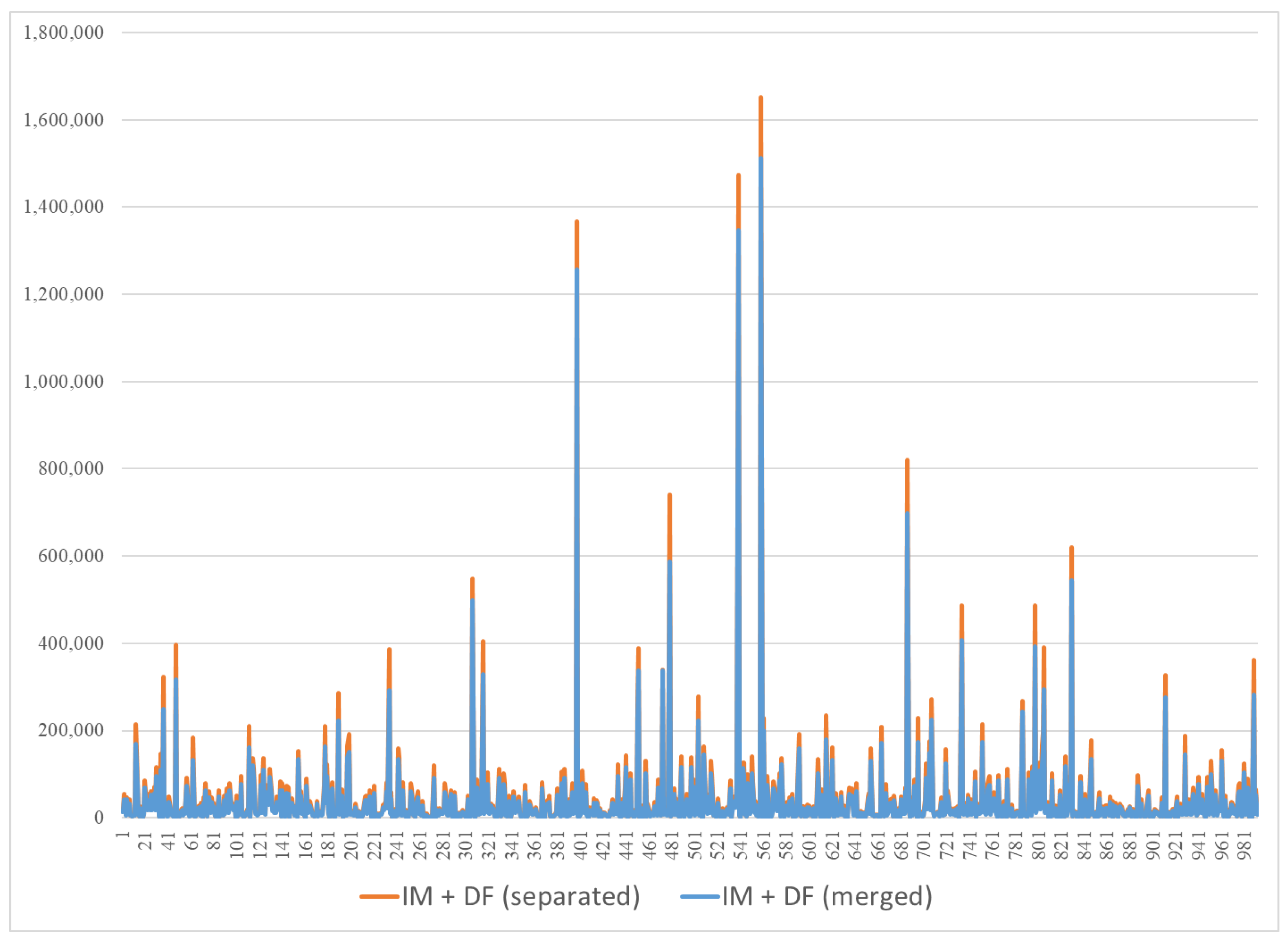
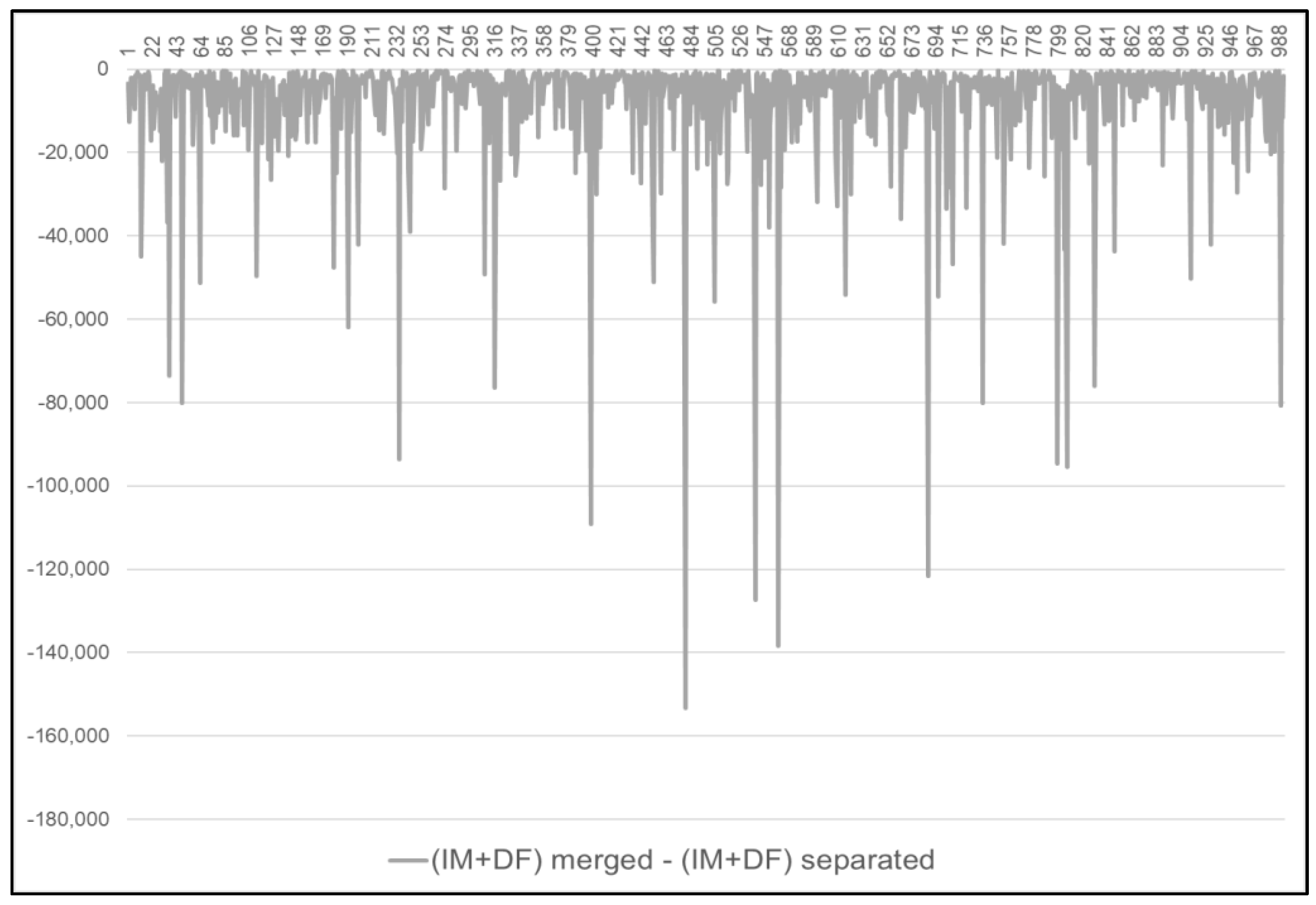
The DF structure is impressive, as well as the whole guarantee system, namely, how the initial margin payment has changed and how the total value of the guarantees (IM + DF) changed. By analyzing the whole guarantee system, we can conclude that the total amount of guarantees is always higher in the separated markets, according to Figure 6. Figure 7 shows the difference between the two guarantee systems, which also shows that the guarantees’ total value always decreases in the merged case.

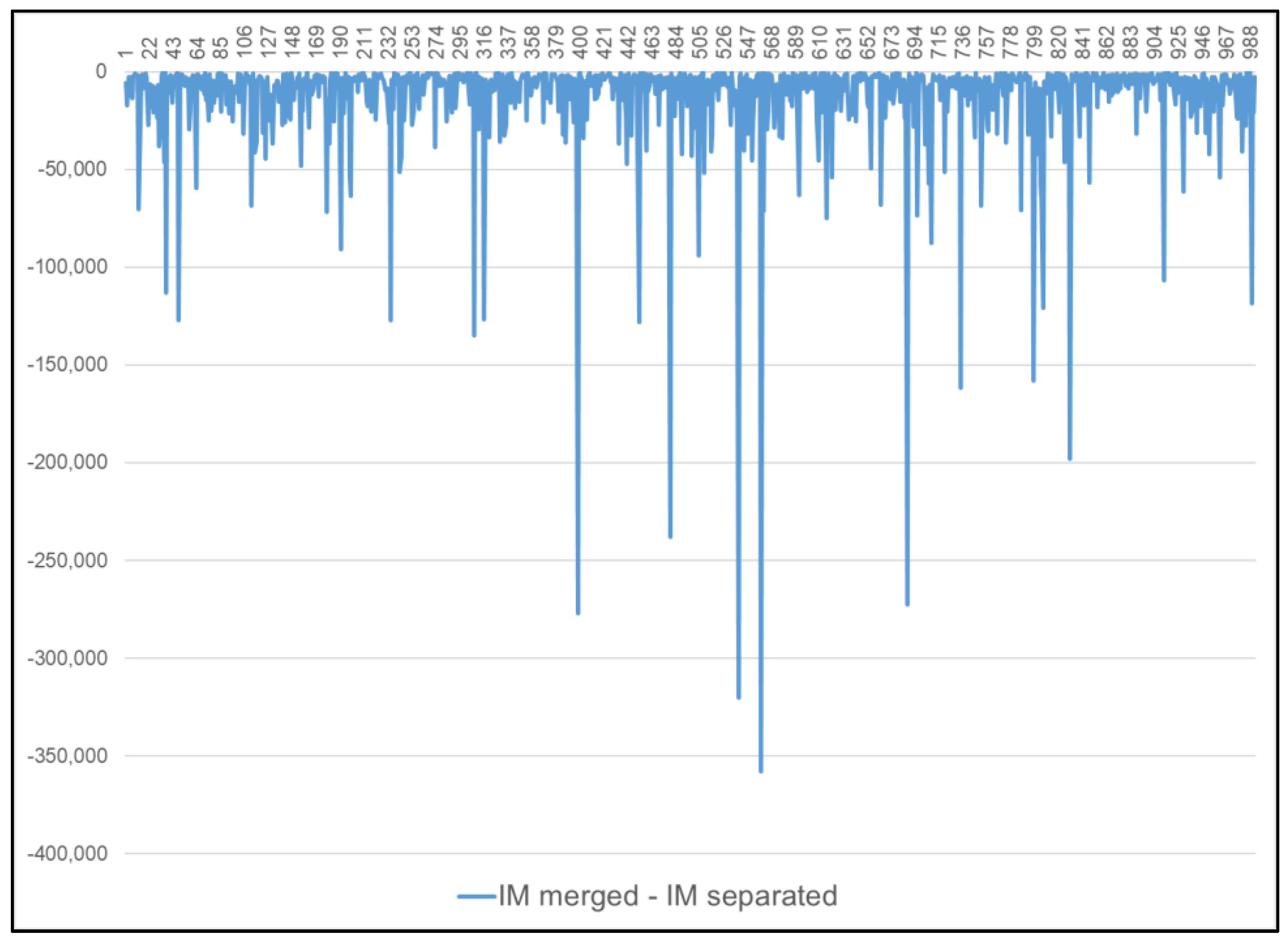
This difference can be the consequence of the portfolio margining on the merged markets since the risk of the spot and derivative markets’ positions cancel out, reflected in the margin values. In every case, the margin is higher on the separated markets than on the merged ones. The difference is presented in Figure 8.

As a robustness check, we ran 1000 simulation a few times more, and the results always had the same patterns as the simulation we have shown.

5. Discussion

Our paper has set up a hypothetical market with one central counterparty, four clearing members, three underlying assets that can be traded on the spot market, and the derivative market as options or futures contracts. We have simulated a 30 year time-series—7500 trading days—for all three assets in order to be able to calculate on the 7500th day the margin requirements and the default fund contributions the clearing members have to pay to the CCP after their open positions. The open positions were built up to show how the cross-guarantee undertaking changes if the CCP merges or separates the guarantee system—the default waterfall—for the spot and derivative markets. One of the members had mainly open short derivative positions, so this clearing member’s portfolio represented a very risky portfolio. Another one had only positions on the spot market; with this, we represented how the cross-guarantee changes between markets. The remaining two had hedged open spot positions with derivative products, so they were active on both of the markets; therefore, we could show how the hedged positions’ advantage from a risk reduction point of view is reflected in the amount of guarantees the clearing members have to pay. We also showed in our paper how the total size and the structure of the guarantee system changes.

The margin requirement and default fund calculation methodology were built on the EMIR regulation, which is the European regulation in force regarding central counterparties. It was important to comply with the EMIR regulation since we wanted to show in our paper whether the merged or the separated default fund structure was more prudent and, consequently, better from a financial stability point of view. The ultimate goal of CCPs is to be shock-resistant by protecting the financial system from one or more default events, preventing a domino effect from emerging, protecting the non-faulty market participant. This assures the smooth day-to-day operation of the system.

Our paper has pointed out why it is essential to carefully build a guarantee system and apply it jointly or separately for different markets. In addition to complying with the regulatory background, it is also crucial to carefully set up the risk management framework for a CCP. The amount of the margin can affect the amount of the default fund, which has different effects on the CCP and the CMs as well, not necessarily positively for both at the same time. Our model is a simplified reality, but the results show how much impact the merged and separated market has regarding cross-guarantee. Our primary goal was to examine how the contribution to the default fund and initial margin changed per each clearing member if we calculated on separated or merged markets and show how the total size of the guarantee system changed. The DF was higher on the merged market in all of the simulated cases. However, analyzing the whole guarantee system, we can conclude precisely the opposite, namely, the total amounts of guarantees are higher in the case of the separated markets. The difference can result from the portfolio margining on the merged markets since the risk of the spot and derivative markets’ positions cancel out, as reflected in the margin values. We also found that the default fund contributions have increased on merged markets—compared to the separated markets—for the clearing members who traded only on the spot markets, so they have to take over some of the other clearing members’ risks. Finally, from a financial stability viewpoint, we would recommend clearing the markets separately since the total value of the guarantees are larger in this case, so the loss-absorbing capacity of the CCP is larger.

6. Conclusions

In this paper, we analyzed how the size and the structure of the guarantee system changes if a central counterparty applied it for merged or separate markets. As a general conclusion, it can be stated that in the separated case, the overall guarantees that are available in the guarantee system are higher; however, the value of the default fund is always larger in the merged case, so the cross-guarantee between the clearing members and markets are more notable. From the clearing members’ perspective, this result makes the merged markets more favorable, since in this case, the trading is cheaper for them, because less collateral is required to be posted. However, because the ratio of the cross-guarantee commitments changes, it is questionable if it is better from a risk-taking point of view for all of the clearing members or not. From the CCPs point of view, if it wants to increase its competitiveness by lowering the guarantees’ value, the merged version should be chosen, but if it wants to have a more prudent guarantee system, the markets should be separated. Finally, from a financial stability point of view, since in the separated case, in more than 60% of the cases, the initial margin was enough to cover potential future losses, the default fund value was 0, it can be stated that the separated markets are more stable andmore stress-resistant, so it should be chosen if the financial stability of the CCP is in focus.

From a regulatory perspective, our recommendation to policymakers, on the one hand, is to follow the more prudent path and specify the operation of the default funds to be handled separately. On the other hand, if the regulator’s most important goal is to handle systemic risk, it must keep a balance between increasing the size of the initial margin and default fund and the liquidity risk it causes for the clearing members. Therefore, it is not evident that the higher initial margin and default fund value is adequate from a systemic risk point of view. This would need further research by extending this analysis with the skin-in-the-game and more complex structure by increasing the number of clearing members, assets, and CCPs in the analysis.

The research’s limitation is that we had only one CCP with four clearing members with small open positions. This could be the basis of future research examining this question using actual portfolios of several clearing members to see if the same phenomena are seen from the cross-guarantees perspective and the guarantee system’s size.

We aim to extend our research to examine the same question on the whole guarantee system level, including the CCP’s contribution to the default fund and the skin-in-the-game.