Article

Adapting the Default Weighted Survival Analysis Modelling Approach to Model IFRS 9 LGD

by
Morne Joubert
†,‡,
Tanja Verster
†,‡,
Helgard Raubenheimer
†,‡ and
Willem D. Schutte
*,†,‡
Centre for Business Mathematics and Informatics, North-West University, Potchefstroom 2531, South Africa
*
Author to whom correspondence should be addressed.
Current address: Internal box 576, Private bag X6001, Potchefstroom 2531, South Africa.
These authors contributed equally to this work.
Risks 2021, 9(6), 103; https://doi.org/10.3390/risks9060103
Submission received: 8 April 2021 / Revised: 12 May 2021 / Accepted: 18 May 2021 / Published: 1 June 2021
(This article belongs to the Special Issue Quantitative Risk Modeling and Management—New Regulatory Challenges)

Abstract

:
Survival analysis is one of the techniques that could be used to predict loss given default (LGD) for regulatory capital (Basel) purposes. When using survival analysis to model LGD, a proposed methodology is the default weighted survival analysis (DWSA) method. This paper is aimed at adapting the DWSA method (used to model Basel LGD) to estimate the LGD for International Financial Reporting Standard (IFRS) 9 impairment requirements. The DWSA methodology allows for over recoveries, default weighting and negative cashflows. For IFRS 9, this methodology should be adapted, as the estimated LGD is a function of in the expected credit losses (ECL). Our proposed IFRS 9 LGD methodology makes use of survival analysis to estimate the LGD. The Cox proportional hazards model allows for a baseline survival curve to be adjusted to produce survival curves for different segments of the portfolio. The forward-looking LGD values are adjusted for different macro-economic scenarios and the ECL is calculated for each scenario. These ECL values are probability weighted to produce a final ECL estimate. We illustrate our proposed IFRS 9 LGD methodology and ECL estimation on a dataset from a retail portfolio of a South African bank.

1. Introduction

Loss given default (LGD) is the percentage loss incurred by a bank (economic loss) when a customer is unable to pay back a loan (customer defaults), and it is commonly acknowledged that LGD is the proportion of the exposure at default (EAD) that remains unpaid in this case. LGD is one of the estimates that a retail bank uses to calculate expected credit loss (ECL) under the recently introduced International Financial Reporting Standard (IFRS) 9 impairment requirements. The estimation of LGD for regulatory capital (Basel) purposes has been widely studied, and common approaches are run-off triangles (Braun 2004, p. 401), beta regression (Brown 2014, pp. 65–66), ordinary least squared approach (Witzany et al. 2012, p. 12), fractional response regression (Bastos 2010, p. 2512), the inverse beta model (Brown 2014, p. 64) and Gamma-related models (Mills 2013; Sigrist and Stahel 2011; Tong et al. 2013). Another approach that is proposed by Joubert et al. (2020), is default weighted survival analysis (DWSA) to directly model LGD. This last mentioned approach is an adaptation of the EAD weighted survival analysis (denoted by EWSA) proposed by Witzany et al. (2012) through the alignment of LGD to the long run default weighted average LGD, and by including negative cashflows and potential over-recoveries.
This research aims to adapt the DWSA methodology in such a way that it satisfies the requirements of IFRS 9, as our research points to limited resources on methodologies to model LGD for IFRS 9 purposes. In this regard, under IFRS 9, Breed et al. (2019) proposed the use of a weighted logistic regression model for LGD, while Krüger et al. (2018) uses a variation of copulas to predict term structures of LGDs and ECLs. Furthermore, Chawla et al. (2016) proposed the use of parametric distributions to model the LGD probability distribution function, while Schutte et al. (2020) used marginal recovery rates that were estimated using run-off triangles. Finally, Grzybowska and Karwański (2019) considered the use of machine learning techniques such as gradient boosting to forecast LGDs using explanatory variables and lagged LGD values.
This paper is organised as follows: First, we will discuss some background in Section 1.1 with specific reference to IFRS 9 and the concepts that need to be addressed to be able to adapt the DWSA methodology for IFRS 9 purposes. Last mentioned IFRS 9 concepts are discussed in Section 1.2. Many adaptations to the DWSA methodology will be required, which is discussed in Section 2. For example, the segmentation used in the DWSA model is the default date and months since default. This needs to be changed to be suitable for IFRS 9, since IFRS 9 LGD models are primarily point in time (PIT) models and calibrated to recent information (Chawla et al. 2016). As opposed to Basel using through the cycle (TTC) models. Section 2 also introduces our proposed new IFRS 9 LGD methodology. The new IFRS 9 LGD methodology is described and fitted to a retail banking portfolio, with the data description given in Section 3.1. The forward-looking IFRS 9 LGD is adjusted for macro-economic scenarios by applying the error correction model (ECM). Several macro-economic variables are considered, with a summary provided in Section 3.2. The complete results following the application of our methodology are provided in Section 4. Finally, in Section 5, we conclude and provide some further research ideas.
SAS software was used for the statistical analyses, model development and data manipulation. However, the proposed methodology is generic and can be coded in any preferred language or software package.

1.1. Background

The International Accounting Standard Board published the new and complete IFRS 9 standard in the form of the document titled IFRS 9 Financial Instruments (IFRS Foundation 2014). This document replaces most of the International Accounting Standard (IAS) 39. It contains impairment requirements that allow for earlier recognition of credit losses. The financial statements of banks must reflect the IFRS 9 accounting standards from 1 January 2018 (European Banking Authority (EBA) 2016, p. 4). Banks have experienced a significant impact on systems and processes due to IFRS 9 (Beerbaum 2015), especially with respect to the assessments of credit risk. For example, capital allocation and risk reporting under Basel require risk estimates for the next period, whereas loan loss provisioning under IFRS 9 covers multiple periods, including the lifetime of financial instruments (Baesens et al. 2016, p. 138).
The IAS 39 makes use of provisions on incurred losses. Learning gained from the 2008 financial crisis showed that expected losses, instead of incurred losses, should be used to calculate the provisioning for banks (Global Public Policy Committee (GPPC) 2016, p. 21). Under IFRS 9, the expected credit losses (ECL) should be equal to an amount equivalent to the lifetime ECL, if the credit risk has risen significantly. When the converse is true, a financial entity may allow for credit losses equal to 12-month ECL. The ECL model is forward-looking and should result in the early detection of credit losses. This will contribute to financial stability (IFRS Foundation 2014, p. 26).
It is now necessary to introduce some notation to progress with the background. The ECL for account i, which is currently at month on book m, is calculated as:
E C L i , m = h = 0 H P D i , m , m + h L G D i , m + h E A D i , m + h 1 + e h .
The marginal P D i , m , m + h is the probability of account i defaulting at month on book m + h , given that the account remained performing until month on book m. L G D i , m + h is the percentage loss given that account i defaults at month on book m + h , and E A D i , m + h is the exposure of account i that defaulted at month on book m + h . The value e is the monthly effective interest rate. LGD is always assessed over the life of the lending exposure (Basel Committee on Banking Supervision (BCBS) 2015, p. 25). The length of the future time horizon, H, for the forward-looking information used in the estimation of ECL will vary between 12 months or the remaining lifetime, depending on the stage of the account. Different modelling approaches are followed for accounts in different stages. An account can either fall into stage 1, stage 2 or stage 3. Stage 1 accounts are performing accounts, and for these accounts, H = m i n ( remaining lifetime ,   12 ) . Stage 2 accounts have significant deterioration in credit risk, but are not in default. Defaulted accounts are in stage 3. We refer to defaulted accounts which are known as nonperforming loans or credit impaired assets in Beerbaum (2015). For accounts in stage 2 and 3, H = remaining lifetime (Aptivaa 2016a). For stage 1, the ECL is not the extended cash shortfall over the 12-month period, but the entire loss on an asset, weighted by the probability that the loss will occur in the next 12 months (Beerbaum 2015). For stage 2 and 3, it is the probability that the loss will occur over the lifetime.

1.2. IFRS 9 Concepts

It is essential to clarify the concepts used in the discussions of the IFRS 9 standard. Since some of these concepts are vastly different from the familiar Basel regulatory capital setting, the following concepts will be clarified in this section: significant deterioration, default definition, staging, lifetime, forward-looking, macro-economic factors and time value of money.
The first concept that is frequently used in IFRS 9 literature is significantly deteriorated. A thirty days past due rule is suggested as a “backstop” when determining if an account has significantly deteriorated since origination (IFRS Foundation 2014, p. 27), i.e., moving from stage 1 to stage 2. The changes in an account’s behavioural score or bureau score, when measured from origination can be used to determine significant deterioration. Accounts that are thirty days past due will be flagged as significantly deteriorated, and the scores are used to select significantly deteriorated accounts from the population that are not thirty days past due.
The default point will occur after the point of significant deterioration. A 90 day past due rule is suggested as a backstop for default, and the default definition should be inline with default definitions already used in other credit risk assessment processes (IFRS Foundation 2014, p. 120). The Basel default definition flags 90 days past due as default and is already deeply embedded in risk management frameworks. The IFRS 9 default definition should therefore be aligned with the Basel default definition. Therefore, as soon as an account becomes nonperforming (i.e., defaults) the account moves from stage 2 to stage 3.
The lifetime of an account is taken as the maximum contractual period over which the accounts are exposed to credit risk (IFRS Foundation 2014, p. 120). For fixed term products, the term of the account can be taken as the lifetime of the accounts, but it is important to recognise all recoveries on the accounts after the write-off point. An analysis should be conducted to measure the amount recovered after the end of the contractual term of the accounts to determine when the lifetime of the account ends. All available information is taken into account when measuring the lifetime of an account that does not have a fixed term. This approach will only function in environments where sufficient history on accounts exists. The historical information that was collected and used for Basel model development purposes should be used.
Forward-looking information is used when modelling ECL (Aptivaa 2016b). The expected loss or the components to determine expected credit losses are forecasted for future time periods, and the sum over the current and future period is used to predict expected losses (Miu and Ozdemir 2017).
Macro-economic factors are modelled onto the time series and different economic scenarios are expressed in terms of the factors included in this model, and a probability is assigned to each of these scenarios (Black et al. 2015). The scenarios are applied to accounts through the macro-economic factors and a probability weighted average expected loss per account is calculated (IFRS Foundation 2014, p. 121).
The time value of money is considered when calculating the expected credit loss. The cashflows on accounts are discounted to the reporting date by applying the current monthly effective interest rate ( e ) (IFRS Foundation 2014, p. 122).
Following the explanation of these frequently used concepts in the IFRS 9 literature, the next section will focus on our proposed methodology to model LGD. We will provide a description of the DWSA modelling approach and how it is used to model the Basel LGD. The adaptation made to the DWSA approach to model the IFRS 9 LGD is then described in Section 2.1.

2. Modelling Methodology: Default Weighted Survival Analysis

The focus of our research is the modelling of LGD directly by estimating LGD as one minus the recovery rate. Witzany et al. (2012) was one of the pioneering authors that proposed a direct modelling approach using EAD weighted survival analysis (EWSA). Thereafter, Joubert et al. (2020) adapted the EWSA concept and proposed the DWSA approach to model LGD for regulatory capital purposes. We provide a brief overview in Section 2.1 and propose an adaptation to the DWSA approach to model LGD for IFRS 9 purposes. In this regard, we provide a description of the DWSA model and the adaptations made to the model to comply with IFRS 9 requirements. Lastly in Section 2.2, we describe the IFRS 9 macro-economic adjustments of the LGD.

2.1. From Basel to IFRS 9 DWSA

The details of the DWSA methodology for Basel purposes can be found in Joubert et al. (2020). A synopsis of the DWSA methodology is provided to facilitate greater understanding of our adaptation. Mathematically the LGD at time of default may be expressed as:
L G D i = E A D i t = 1 T w D C F i , t E A D i ,
where D C F i , t = C F i , t 1 + e t is the discounted future cashflows for account i at time t and E A D i , the EAD for account i. The recovery time, t { 1 , , T w } , for a defaulted account, i, is measured in months. Cashflows C F i , t are calculated as the difference between the present account balances versus account balances in the previous month, adding back the interest and the fees and subtracting the amount written off. The post write-off recoveries represent recovery or additional expense amounts post the write-off date, which are added to the cashflows (Witzany et al. 2012, p. 8). All accounts with recovery information up until time T w are deemed to have complete recovery information. The time when the recovery process ends for account i will be denoted by t i , e n d . The recovery process is completed if t i , e n d < T w , i.e., if an account closes before T w . Inversely, the recovery process is incomplete if T w t i , e n d .
A survival curve, S t , i = 1 P ( T < t ) is defined as the (unrecovered) proportion of E A D i that remains in default up to a specific recovery time t for account i. This survival curve follows a related expression as Equation (2) except that the summation is only to recovery time t. The Kaplan-Meier estimate, S ^ ( t , i ) , can then be used to estimate the empirical value of the survival curve calculated from the data. To perform the empirical calculation, the data needs to be constructed in a specific way when applying the DWSA methodology to incorporate censoring, incomplete records, unrecovered amounts, etc. For more information on implementation and dataset construction, see Joubert et al. (2020).
Following the construction of the empirical survival curve, a decision must be made on the modelling methodology. In this regard, the Cox proportional hazard model (CPHM) is a nonparametric model that could potentially be used in a regression setting (Miller 2011, p. 119). The general form of the CPHM is given by:
S t , x i = S 0 t e x p ( x i β ) ,
where x i is the covariate values for account i and β is the vector of unknown regression parameters associated with the vector of covariates. The weighted survival curve at time t in default contains a component S 0 ( t ) known as the baseline hazard function. The baseline hazard function can be estimated using the Kaplan–Meier estimate of the portfolio (i.e., no distributional assumptions were made) and serves as a reference point to describe the risk at time t for accounts with covariates x i = 0 . For accounts with x i 0 , the baseline, S 0 ( t ) , is shifted by e x p ( x i β ) . For a detailed account of the use of survival analysis in a credit risk setting, consult Smuts and Allison (2020). The loss given default for account i at default is then calculated as:
L G D i = S T w , x i S 0 , x i .
Since the DWSA modelling methodology is proposed as a potential model for the Basel LGD, we now need to illustrate the adaptations required to move towards a methodology used to model the IFRS 9 LGD. The adaptations to the DWSA approach are divided into four sections: segmentation, reference period, LGD calculation and macro-economic model.
The IFRS accord stipulates that forward-looking information must be used when estimating the IFRS 9 LGD. L G D m , the loss given that the account defaults at month on book m, is calculated from historical data. The segmentation for the DWSA approach is adapted from using the default date and months since default, to using the month on book, m, and the application date.
The IFRS 9 LGD is calibrated to recent information. The reference period for the IFRS 9 LGD is illustrated in Figure 1 and the example shows that the reference period falls between the two blue dotted lines where the information for the months January 2016 to December 2017 is used. Furthermore, Figure 1 illustrates how the population for m = 4 is selected. All accounts that default at m = 4 (e.g., account A and C in Figure 1) are considered. The exposure at entry into the reference period and the cashflows within the reference period, for accounts defaulting at m = 4 are considered to calculate L G D 4 .
The exposure at entry into the reference period is used to model the IFRS LGD; this replaces the exposure at default used for modelling the Basel LGD. The cashflows used for the Basel LGD span the workout period. The cashflows for the IFRS LGD span the recent reference period as displayed in Figure 1.
While the Basel LGD under the DWSA approach for account i at any point t in default may be calculated using Equation (4), the IFRS 9 LGD for account i that defaults at a specific month on book m is:
L G D i , m = D E i , m n = m + r i + 1 m + r i + R D C F i , n D E i , m ,
where D E i , m = E A D i , m n = m + 1 m + r i D C F i , n , is the value of the exposure at entry into the reference period for account i. Please note that E A D i , m is equal to E A D i , the EAD at the default date, as in the Basel LGD calculations. The reference period is the area between the two blue dotted lines in Figure 1, and the length of the reference period is indicated by R. Practical experience has shown that 12 to 24 months could be used for R. Still, it is greatly dependant on the legal or business environment and the nature of the product. One could also achieve a good estimate of this period during data inspection by investigating when the recovery cashflows stabilise. In Figure 1, also observe that account i enters the reference period at time m + r i . Cashflows on account i occurring in the reference period are discounted to the time of default occurring on month on book m, i.e., D C F i , n = C F i , n 1 + e n m . Cashflows C F i , n are calculated as the difference between the present account balances and the account balances in the previous month, adding back the interest and the fees and subtracting the amount written off. Post write-off recoveries are added to the cashflows and are the additional expenses or recoveries after the write-off event (Witzany et al. 2012, p. 8).
Similarly, as in Joubert et al. (2020), a special dataset needs to be constructed. Each cashflow in the reference period will result in a separate record, with the unrecovered amount as the last record. An indicator variable for censoring is added to indicate if the account does not have information until the end of the reference period.
The survival curve, S ( m , r , i ) , is then defined as the proportion of the exposure at entry into the reference period that remains in default from a specific time r ( m + r i < r < m + r i + R ) until the end of the reference period, for account i that defaults at month on book m. The Kaplan-Meier estimate for this survival curve is the empirical value calculated from the data and can be expressed as:
S ^ m , r , i = D E ^ i , m n = m + r i + 1 m + r i + r D C F ^ i , n D E ^ i , m .
The survival curve for the segment of account that defaulted on month on book m is then calculated as:
S 0 ^ m , r = D E ^ m n = m + r i + 1 m + r i + r D C F ^ n D E ^ m ,
where D E ^ m = i I m D E ^ i , m and D C F ^ n = i I m D C F ^ i , n with I m indicating the set of accounts defaulting at month on book m. The resulting CPHM is then derived from Equation (3) as follows:
S m , r , x i = S 0 m , r e x p ( x i β m ) ,
where S 0 m , r is the baseline survival curve. The CPHM is then fitted for each month on book segment and the LGD for account i that defaults at month on book m, is given by:
L G D i , m = S m , m + r i + R , x i S m , m + r i , x i .

2.2. Macro-Economic Adjustments

The forward-looking LGD values ( L G D i , m + h ) in Equation (1) that is used to calculate E C L i , m for each account i are then derived from Equation (9). However, these LGD values need to be adjusted for different macro-economic scenarios before application.
The IFRS 9 accord (IFRS Foundation 2014, p. 189) requests banks to incorporate forward-looking macro-economic information into their estimation of lifetime expected credit losses. Various macro-economic scenarios are expressed in terms of macro-economic factors, and probabilities are assigned to these scenarios. Therefore, the three components used in the ECL calculation need to be modelled with respect to the macro-economic factors and will be discussed next.
To adjust for different macro-economic scenarios, the L G D i , m values in the ECL calculation are expressed as a time series. Let L G D c , i be the LGD for account i, assuming the account defaults in calendar month c:
L G D c , i = S m c , m c + r i + R , x c , i S m c , m c + r i , x c , i ,
where S m c , r , x c , i = S 0 m c , r e x p x c , i β m c and m c is the month on book for account i at calendar month c. Please note that x c , i is the set of covariates for account i at calendar month c and β m as fitted before, i.e., the fitted model is applied to the portfolio on calendar months c = 1 , , C resulting in a time series of LGDs. For every calendar month c the weighted average LGDs are calculated, with the weights equal to the EADs, to obtain a portfolio LGD,
L G D c = i L G D c , i × E A D c , i i E A D c , i ,
where E A D c , i is the EAD for account i at calendar month c.
To incorporate the macro-economic factors into the time series, an ’Error Correction Model’ (ECM) (Engle and Granger 1987) is implemented using co-integration and error correction. For a detailed discussion on the implementation aspects of the ECM, see Mohamed (2010). In brief terms, the ECM may be implemented using four steps (Mohamed 2010). The first step is to determine whether all the time series (LGD values and macro-economic variables) are integrated of the same order (Mohamed 2009b). The second step is to demonstrate that the time series is co-integrated (Mohamed 2009a), implying a stationary linear combination between the two non-stationary time series (Granger 1981). The third step is to generate residuals by regressing the LGD values on the macro-economic variables. The last step is to enter the lagged residuals from the third step into a regression of the LGD differences (due to the macro-economic differences of the previous time period).
The augmented Dicky-Fuller (ADF) test is used in the first step to test for stationarity (Mohamed 2009b). To test for co-integration in the second step, an ordinary least squares regression is done between the LGD and the macro-economic variables. If the error terms from the regression are stationary, it is concluded that co-integration exists (Mohamed 2009a). The regression model in the third step can be defined as follows:
L G D c = α 0 + α z c + ε c
where z c = { z 1 , , z n } is the n macro-economic variables, α 0 and α = α 1 , , α n are the parameters and ε c the residuals. The ECM in step four is expressed as:
Δ L G D c = ϕ 0 + ϕ Δ z c + ϕ n + 1 ε c 1 + ε c ,
where Δ L G D c = L G D c L G D c 1 and Δ z c = z c z c 1 . ϕ 0 , ϕ = ϕ 1 , , ϕ n , ϕ n + 1 are the parameters, ε c 1 is the lagged residual from step three and ε c is the error term. Please note that the term ϕ Δ z c in the model may be extended to include different lags. Variable selection will be typically done using stepwise selection. Alternative models (to the ECM) could also be used to incorporate the macro-economic factors into the time series, such as regression models with time series errors (Tsay 2014, p. 90) or VARMAX models (Gomez 2019, pp. 121–72). These are, however, some future research ideas.
In general, the term ε c captures all other factors that influence the dependent variable L G D c other than the independent variable z c (this may be referred to as the ‘long-term’ error). In this sense, ECM can be interpreted as a method to combine the long run co-integrating relationship between the level variables and the short run relationship between the first differences of the variables (Mohamed 2010).
Forecasted macro-economic values for z c can be obtained in various ways. In our case, we used the forecasts from Moody’s Analytics. Internal forecasts can also be used, or any other source deemed appropriate. For each macro-economic variable, an upturn (optimistic), downturn (pessimistic) and base case forecast is obtained. Let z c u be the optimistic scenario, z c b the base scenarios and z c d the pessimistic outcome. Given that actual data are used as far as it is known, the values of the three scenarios described above will be the same up to the point where the forecast starts. These variables are then used as input into the ECM to estimate L G D c u , L G D c d and L G D c b , i.e., an optimistic-, pessimistic- and base LGD by calendar month, respectively. The average of each scenario’s LGD values is calculated over the forecasted period. It is now required to calculate the value of a scalar that can be used to shift the L G D i , m from the base scenario to either the optimistic, or the pessimistic scenario, respectively. In this regard, two scalars are calculated as follows:
s c a l a r u = c = 1 f L G D c u c = 1 f L G D c b
and
s c a l a r d = c = 1 f L G D c d c = 1 f L G D c b ,
where f is the length of the forecast window.
A optimistic-, pessimistic- and base LGD by month on book are required for the ECL calculation. The above scalars are used to shift L G D i , m to an optimistic L G D i , m u and a pessimistic L G D i , m d where L G D i , m u = L G D i , m × s c a l a r u and L G D i , m d = L G D i , m × s c a l a r d .

3. Case Study Data Description

The proposed methodology discussed to date was applied to actual data received from a bank. Although little information will be provided due to the confidential nature of the data, the construction of the empirical LGD will be provided, as well as a description of the macro-economic variables that were used in the ECM.

3.1. Empirical LGD

The development dataset that is required to model the IFRS 9 LGD includes the exposure at the entry into the reference period and values for all cashflows during the reference period. The default flag is needed to determine if an account is in default as at a specific month on book; the default flag and month on book indicator are stored on the development dataset. The account number, application date, closed date, effective interest rate and month are stored. The covariates, x , i.e., used in the CPHM include behavioural-, customer-, and geographical- information and are added to the development dataset.
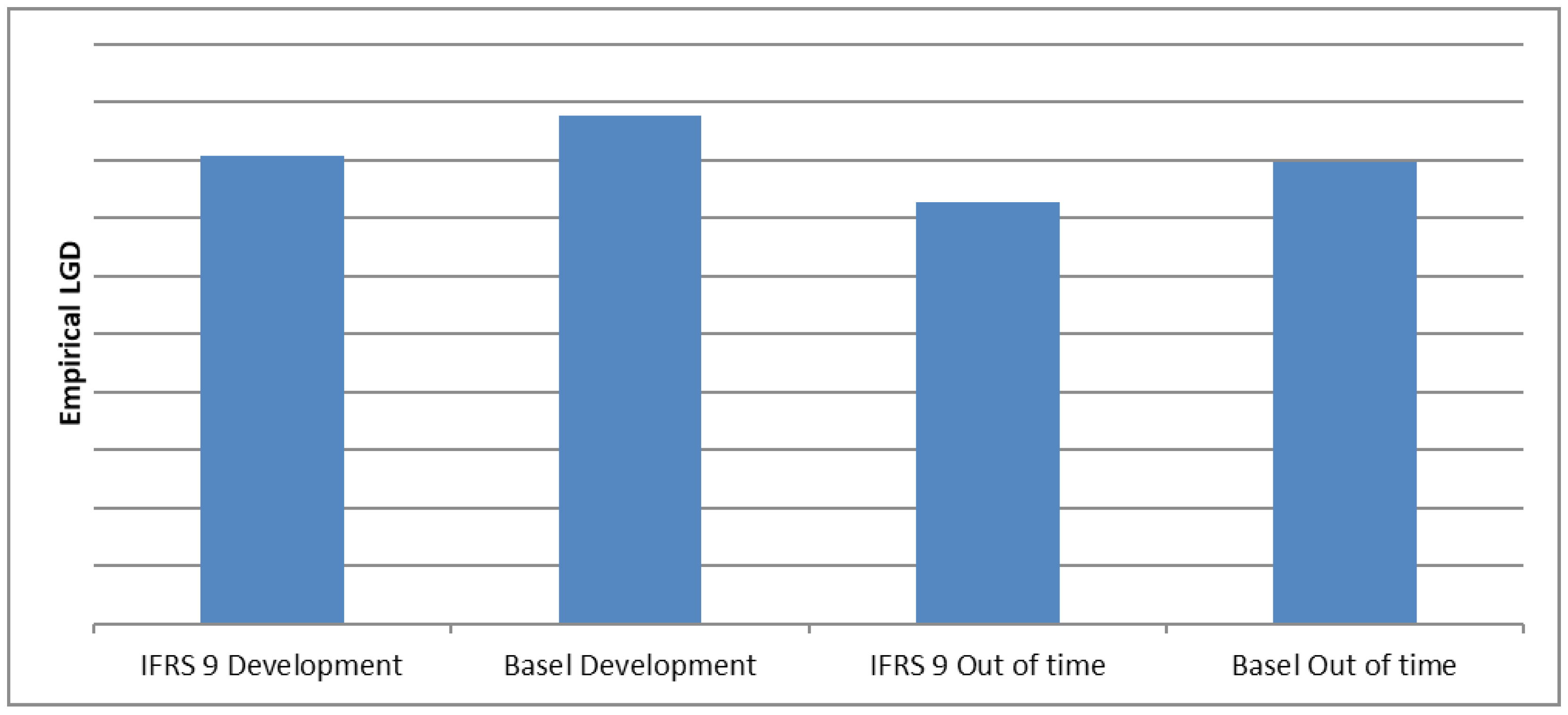
Data for an unsecured retail product from a South African bank are used in this paper. The development dataset had 134,741 defaulted accounts, and the out of time dataset had 132,642 accounts. Data from January 2005 up until December 2017 was considered for development. The development reference period for the IFRS 9 LGD was selected as the most recent 24 month period available, and the out of time sample consisted of the preceding 24 months. The empirical IFRS 9 LGD for the development- and out of time dataset are displayed in Figure 2. The average % LGD for the “Retail other” class across the four major banks in South Africa ranges between 32% and 41% as published in their 2019 Basel Pillar III regulatory disclosure reports, e.g., Nedbank (2019). Please note that these levels differ over economic cycles, institutions and products. However, these levels can be used as an indication of the level of the % LGD and should provide the reader with an impression for the axis in the graphs. The empirical IFRS 9 LGD is calculated over a recent 24 month reference period, as was discussed in Section 2.
The exposure used for this IFRS 9 calculation is the exposure at the beginning of the reference period. This is in contrast to regulatory models where the exposure at default is used. IFRS9 cashflows are summed over the reference period, whereas Basel is summed over the workout period. The Basel LGD is therefore expected to be higher than the IFRS 9 LGD. The IFRS 9 LGD is calculated by subtracting the sum of the discounted cashflows over the reference period from the exposure at entry into the reference period, divided by the exposure at entry into the reference period. The Basel LGD is calculated by subtracting the sum of the discounted cashflows over the workout period from the exposure at the default point, divided by the exposure at the default point. The IFRS 9 LGD for accounts i that defaults at a specific month on book m is:
L G D i , m ^ = D E i , m ^ n = m + r i + 1 m + r i + R D C F i , n ^ D E i , m ^ ,
where D E i , m ^ = E A D i , m ^ n = m + 1 m + r i D C F i , n ^ , is the value of the exposure at entry into the reference period for account i, and E A D i , m ^ is equal to E A D i ^ , the EAD at the default date (similar to the Basel LGD). The portfolio IFRS 9 LGD is calculated as:
L G D m ^ = D E ^ D C F * ^ D E ^ ,
where D E ^ = m i D E i , m ^ and D C F * ^ = m i n = m + r i + 1 m + r i + R D C F i , n ^ . The empirical Basel LGD is calculated over a workout period of 60 months and is expressed as:
L G D ^ i = E A D ^ i t = 1 T w D C F ^ i , t E A D ^ i ,
where E A D ^ is the exposure at default for account i. The portfolio’s empirical Basel LGD is:
L G D ^ = E A D ^ D C F ^ E A D ^ ,
where E A D ^ = i E A D ^ i and D C F ^ = i t = 1 T w D C F ^ i , t . The IFRS 9 development sample is constructed from the recent 24 month reference period and the out of time sample from the 24 month period preceding the development sample. The Basel development sample is constructed from the 24 month time period where benign economic conditions were prevalent. The out of time data were constructed from the 24 month time period preceding the development sample. The LGD values in all figures depicting LGD levels are left out due to the confidential nature of the data.

3.2. Macro-Economic Variables

The second part of the data description is focused on the macro-economic variables that were used in the ECM. The following macro-economic variables were considered during the implementation of the ECM:
  • The consumer price index (CPI) is the increase in the level of prices of a representative basket of goods purchased by consumers and households. This measures how much purchasing power in a country is eroded by price increases.
  • The ratio of debt to disposable household income (DDHI) is a measure that indicates the ability of households to repay their debts. This measure is derived by dividing total monthly household debt by monthly income.
  • The debt service ratio (DSR) is the proportion of household income that is spent on covering existing debt agreements.
  • The M3 money supply is the money supply in circulation and indicates a country’s liquid money supply.
  • The gross domestic product (GDP) is an indication of the total local production of the economy.
  • The nominal house price index (NHPI) is an index of the average house price level, without adjusting for inflation.
  • The real house price index (RHPI) is an index measuring the average house price level, which adjusts for inflation.
  • The prime interest rate is the rate at which the banks of South Africa lend money to customers.
  • Debt affordability is the ratio of government debt relative to the resources available for repaying that debt.
  • The leading indicator is a forecast of the general health of the South African economy.
  • Rand dollar exchange rate is the price of one dollar in rand terms.
  • Liquidity spread is the premium that flows to a party willing to provide liquidity to a party that is demanding it.
This concludes the description of the case study data, and the following section will present the results obtained following the application of the methodology.

4. Results

In this section, we will present the results following the application of our proposed methodology as described in Section 2 to the data described in the previous section. The results as presented separately for the IFRS 9 LGD model and the macro-economic model. The aim of the application of our proposed methodology is not to provide the reader with information on the LGD characteristics of the portfolio, but to provide evidence of the usefulness and reliability of the proposed methodology.

4.1. IFRS 9 LGD Model

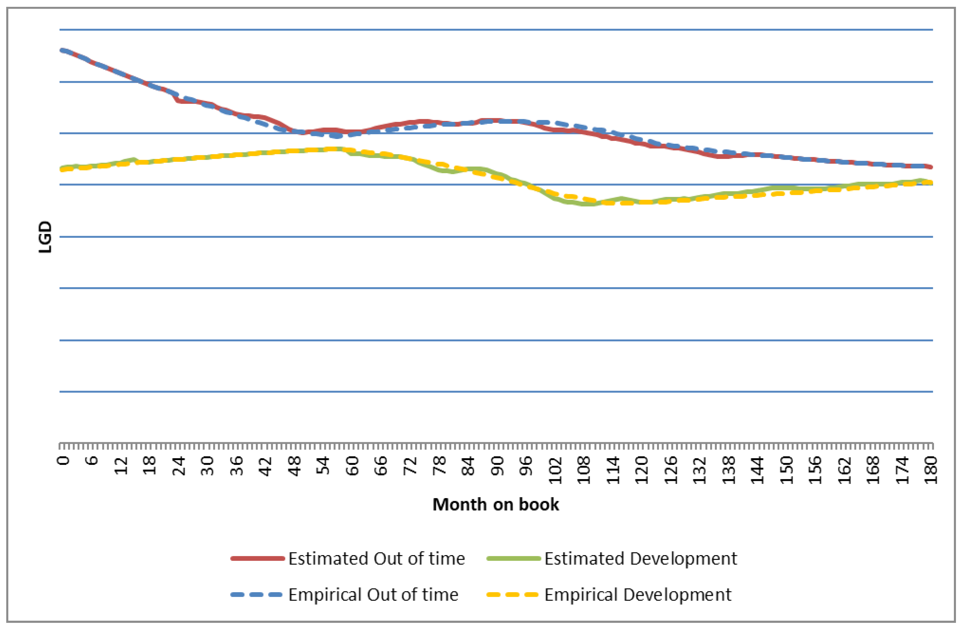
The IFRS 9 LGD is calculated by applying the methodology described in Section 2 to a retail credit portfolio of one of South Africa’s major banks. The model was fitted to the development reference period for a portfolio and then applied to the same portfolio using both the development and out of time reference period. The empirical and estimated LGD values for each month on book are displayed in Figure 3. A difference in the overall level and directional movement of the development LGD and out of time LGD is observed. The reasons for these movements are provided in the discussion of Figure 4. A low number of accounts were observed where months on book is more than 180, causing the LGD values to be volatile past this point (not shown). The LGD value at months on book equal to 180 will therefore be used for accounts more than 180 months on book.
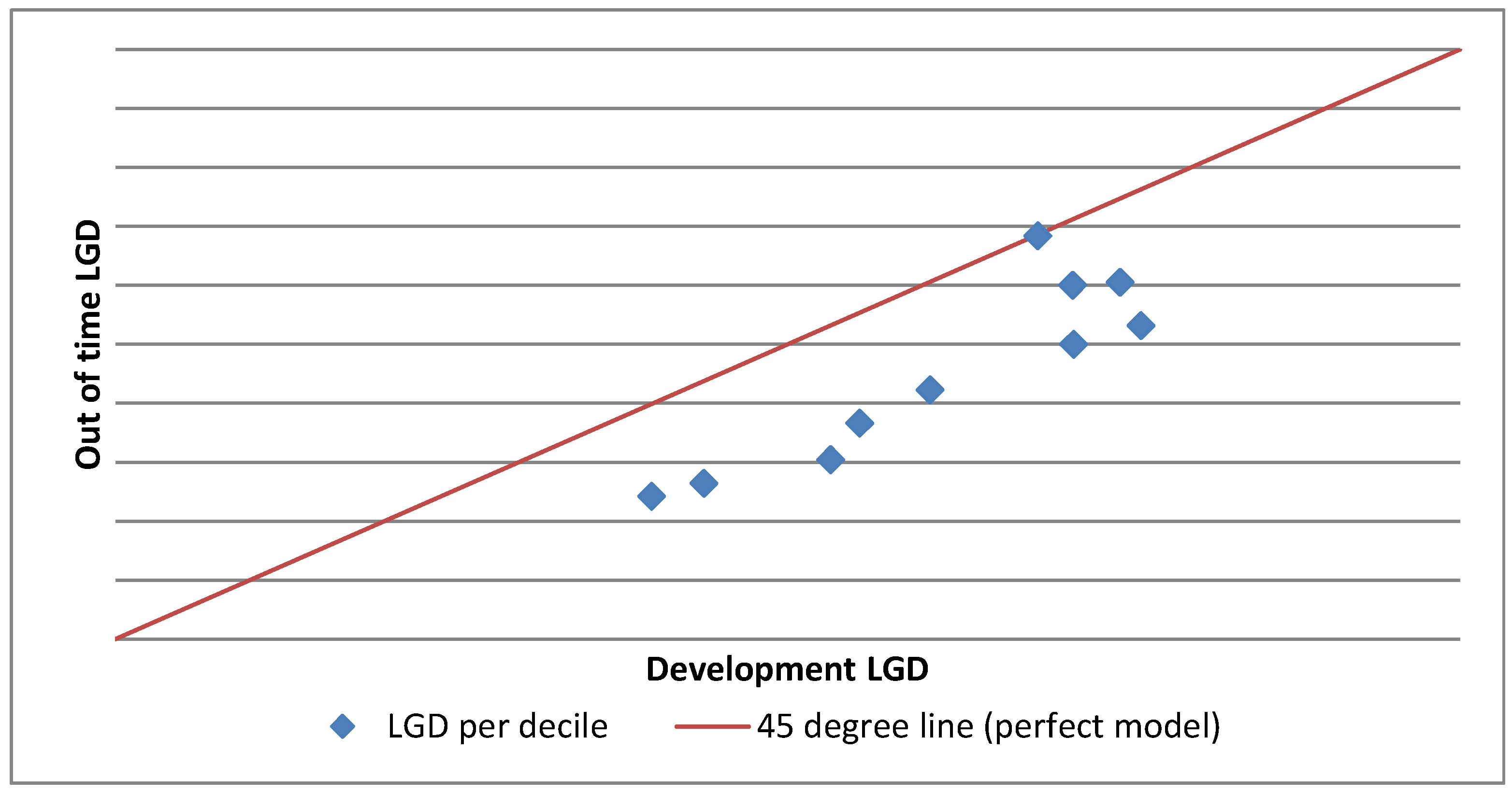
The IFRS 9 development and out of time LGD values are compared in Figure 4. The development LGD was sorted in descending order and placed in deciles. The average out of time LGDs are compared to the average development LGDs per decile, and plotted in this figure. A 45 degree line is also depicted to indicate the situation where the development and out-of-time LGDs are equal, i.e., perfect model. The development LGD values are lower than the out of time LGD values. The development reference period is the most recent 24 months and the out of time reference period is the preceding 24 months. The differences in strategies, customer behaviour and macro-economics are causing the LGD for these periods to be different. IFRS 9 LGD values are PIT in nature and movements in these curves over time are therefore anticipated. The PIT IFRS 9 LGD values will accordingly be updated frequently to ensure that recent information is reflected in the LGD and ECL values. The movement between the development and out of time LGD values are therefore expected.
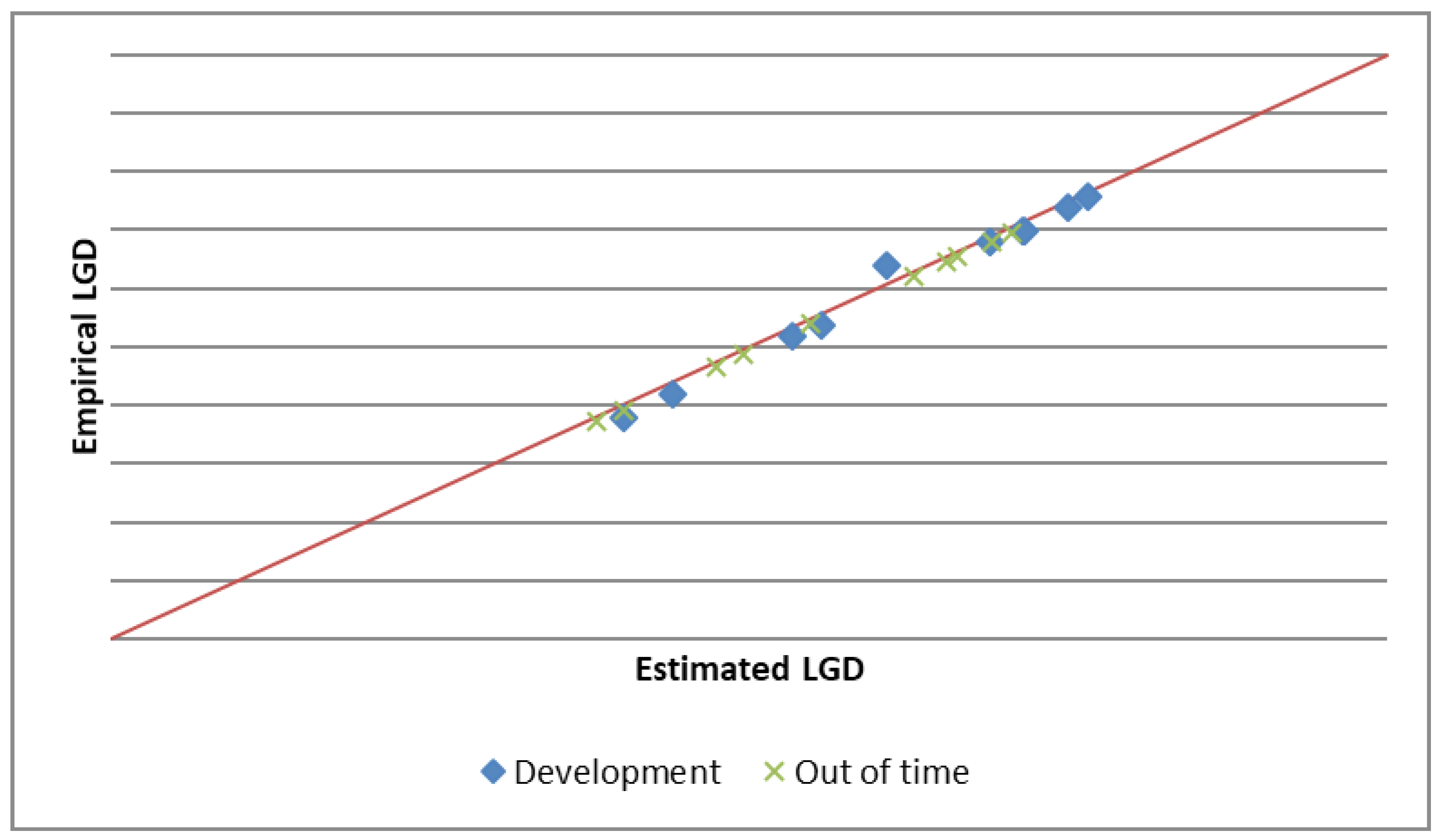
Figure 5 compares the estimated vs the empirical IFRS 9 LGD values for both the development period and the out of time reference period. The estimated LGD was sorted in descending order and placed into deciles. The average estimated LGD vs average empirical LGD per decile are plotted in Figure 5 and shows that the estimated IFRS 9 LGD are close to the empirical IFRS 9 LGD values for both reference periods. This points towards the fact that the modelling methodology and adjustments made produce results that are accurate and reliable over time.

4.2. Macro-Economic Model (ECM)

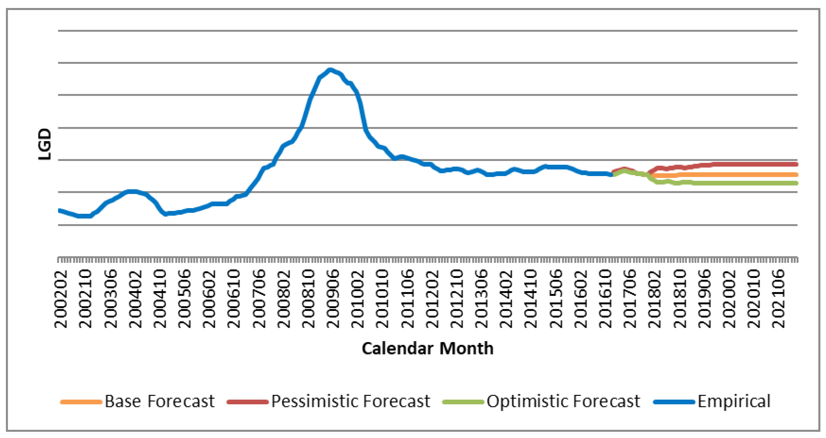
The values for L G D c , i are displayed in Figure 6. A time series of macro-economic variables was fitted to the LGD curve in Figure 6, with these values as the target in the ECM. Stationarity- and co-integration tests were performed, followed by the fitting of the ECM.
The first step of the ECM was performed to determine whether all the time series were integrated of the same order. The ADF test was used to test for stationarity. The regression procedure in SAS was used to perform the ADF test, although any other software package can be used. The t-values from the regression procedure were compared to the t-statistic with a confidence level of 0.01. The t-statistic is equal to −3.524233 when a confidence level of 0.01 is considered. The t-values for the macro-economic variables are given in column two of Table 1. Each of these t-values is greater than the t-statistic value of −3.524233. We fail to reject the null hypothesis and conclude that the macro-economic variables are non-stationary when no differencing is performed. The first difference was taken and the ADF test applied to test if the first difference is stationary. The t-values for the differenced macro-economic variables are in column three of Table 1 and are less than the value of the t-statistic, −3.524233. These variables are therefore stationary and integrated of order one.
The second step was performed to demonstrate that the time series are co-integrated. An ordinary least squares (OLS) regression with L G D c as the target and the macro-economic variables as the independent variables was performed and the residuals stored. These residuals were then tested for stationarity by performing the ADF test. Column four of Table 1 contains the t-values for the errors. This ADF test showed that the error terms are stationary and conclude that L G D c and the macro-economic factors are co-integrated.
The ECM was fitted with Δ L G D c , i as the target. The independent variables were the first difference of the macro-economic factors and the lagged error term from the previous regression. The macro-economic variables listed in Section 3.2 and their lags were considered for the long-term and short-term effect in the ECM. Lags 1 to 12 were taken for the first difference of each of the macro-economic factors. These were entered into a stepwise regression with an entry and exit significance level of 0.05.
The third step was to generate residuals by regressing the LGD values on the macro-economic variables. The parameter estimates, lags and variance inflation factor for the variables are given in Table 2.
The final step was to enter the lagged residuals from step three into a regression of the LGD differences on the macro-economic differences of the previous time period. The parameter estimates, lags and variance inflation factor for the variables are given in Table 3. The R 2 statistic is not provided as the interpretation is not straight forward. Since the regression does not contain an intercept term (the regression line is forced to runs through the origin), it implies that the R 2 statistic is not defined in the standard way (Mohamed 2010) and is therefore not comparable to the usual R 2 statistic calculated from a regression with an intercept.
The leading indicator and debt affordability entered the long-run portion of the ECM and will have a long term effect on the forecasted LGD. The GDP, DDHI and prime interest rate has a short term effect on the forecasted LGD, since these variables entered the short term portion of the ECM.

4.3. Macro-Economic Scenarios

The fitted ECM is applied to the forecasted covariates of the optimistic-, pessimistic- and base macro-economic scenarios. The covariates for these scenarios are z c u , z c d and z c b and the resulting LGD by calendar months are L G D c u , L G D c d and L G D c b , respectively. These LGD values are displayed in Figure 7.
The values for s c a l a r u and s c a l a r d (see Equations (14) and (15)) were calculated from the forecasted portions of the LGD values that are displayed in Figure 7. The LGD by month on book values for each of the three macro-economic scenarios were calculated as L G D i , m u = L G D i , m × s c a l a r u and L G D i , m d = L G D i , m × s c a l a r d .
These LGD values, together with a macro-economic adjusted PD and EAD, were entered into Equation (1) to calculate an ECL value for each scenario. A marginal PD model using a frequentist approach was used, with similar macro-economic adjustment as in the LGD model. The same set of macro-economic variables were considered and forecasts were obtained from Moody’s analytics. The EAD is estimated using the amortisation schedule of each account with discounting. The probability of each scenario occurring are provided and are used to calculate a weighted ECL value. The percentage increase in the macro-economic adjusted IFRS LGD, percentage ECL increase and scenario weights for each of the macro-economic scenarios are given in Table 4. These values can be interpreted as the quantification of the contribution of using macro-economic adjustments in the model. Please note that while the LGD increase by 5.17% in the optimistic scenario, the ECL increase is less. The ECL increase is more than the PD increase (3.29%) for the optimistic scenario. We observe that the LGD for the pessimistic scenario increased by 4.03%. The PD increased by 2.07% and ECL by 3.27%. In terms of the macro-economic variables, the GDP, Prime interest rate and Debt affordability variables were significant in the PD and LGD models. In Figure 6 and Figure 7, there is evidence of a time period where adverse economic conditions were experienced. The fact that we used PIT estimates and incorporated macro-economic conditions imply that the IFRS 9 model will be procyclical (Novotny-Farkas 2016). It is expected, though, that the procyclicality of this IFRS 9 model will be lower than a model developed under IAS 39 due to the use of staging of accounts to recognise potential losses at an earlier stage.
As mentioned in the introduction, IFRS 9 LGD models are primarily PIT models. Generally, there are two risk philosophies: TTC versus PIT (Taylor 2003). PIT and TTC approach the issue of cyclicality quite differently, but there is value in both. PIT focuses on current events, while TTC recognises cyclicality as an innate and self-correcting characteristic whose ill effects are absorbed over time (Taylor 2003). According to Baesens et al. (2016) there is quite a controversy regarding procyclical risk measures. Banks often find it challenging to raise capital (or raise provisions) during economic downturns. The use of PIT model leads to procyclical capital and impairment requirements that may further exacerbate economic downturns. However, it must be noted that PIT models are more accurate than TTC models in the sense that TTC predictions do not match actual default rates (Siddiqi 2017). TTC models have the advantage of creating stable predictions (Siddiqi 2017), with PIT models creating more volatile predictions. Typically PIT models are built using all the relevant important information, and TTC models generally exclude cyclical variables (Taylor 2003).

5. Conclusions

Survival analysis is one of several methods used to predict loss given default (LGD) for Basel regulatory purposes. When using survival analysis to model LGD, one proposed methodology is the default weighted survival analysis (DWSA) method. In this paper, we adapted the DWSA method (used to model the Basel LGD) to estimate the LGD for IFRS 9 impairment requirements. This IFRS 9 LGD is used in the calculation of the expected credit loss (ECL) as per the IFRS 9 accord. The proposed IFRS 9 LGD methodology that is described in this paper makes use of survival analysis to estimate the LGD by making many adaptations to the Basel DWSA approaches. These adaptations were divided into four sections: segmentation, reference period, LGD calculation and macro-economic model. The Cox proportional hazards model (CPHM) allows for a baseline survival curve to be adjusted to produce survival curves for different segments of the portfolio. The DWSA methodology allows for over recoveries, default weighting and negative cashflows. The forward-looking LGD values are adjusted for macro-economic scenarios. An error correction model (ECM) was used to predict a macro-economic model. An ECL value is calculated for different macro-economic scenarios. These ECL values are then probability weighted to produce a weighted ECL.
The proposed survival analysis methodology to produce the IFRS 9 LGD was validated and tested on a South African retail bank portfolio by comparing the empirical and estimated LGD by deciles. All the necessary stationarity and co-integration tests were performed when fitting the ECM, and the results are promising concerning the methodology’s accuracy. As expected with PIT estimates and models that incorporate macro-economic variables, procyclicality is present. As stated, there are two approaches to handle cyclicality: either PIT or TTC. PIT variability causes procyclical movements in loss provisioning. In contrast, a TTC philosophy let the capital or provisions absorb the ups and downs of actual losses around the long-run expected level (Taylor 2003). As used in IFRS 9, a PIT philosophy can create volatile impairment of loans if the economy fluctuates, and this might create financial statements that are not stable over time. Banks prefer more stability in financial statements, specifically for the sake of shareholders. Furthermore, the inherent PIT philosophy of IFRS 9 typically results that in bad times of the economic cycle, provisions must be made higher and puts the bank in a difficult situation to react to the next cycle.
Future research ideas include a focus on the IFRS 9 PD component that is used to calculate the ECL. In this regard, it might be prudent to investigate whether Basel PD modelling methodologies could be adapted for IFRS 9. Otherwise, survival analysis, machine learning and behavioural scorecard techniques can be considered to model the IFRS 9 PD. Alternative models to incorporate the macro-economic factors into the time series can also be investigated, such as regression models with time series errors or VARMAX models.

Author Contributions

All authors contributed equally to this work. All authors have read and agreed to the published version of the manuscript.

Funding

This work is based on research supported in part by the Department of Science and Innovation (DSI) of South Africa. The grant holder acknowledges that opinions, findings and conclusions or recommendations expressed in any publication generated by DSI-supported research are those of the authors and that the DSI accepts no liability whatsoever in this regard.

Institutional Review Board Statement

Not applicable.

Informed Consent Statement

Not applicable.

Acknowledgments

The authors would like to acknowledge the input from anonymous referees that greatly improved the quality of the manuscript.

Conflicts of Interest

The authors declare no conflict of interest.

References

  1. Aptivaa. 2016a. Building Blocks of Impairment Modeling (Issue 02). Available online: https://www.academia.edu/30200858/Building_Blocks_of_Impairment_Modeling (accessed on 4 March 2020).
  2. Aptivaa. 2016b. Cash Shortfall and LGD Two Sides of the Same Coin. Available online: http://www.aptivaa.com/blog/cash-shortfall-lgd-two-sides-of-the-same-coin/ (accessed on 4 March 2020).
  3. Baesens, Bart, Daniel Rösch, and Harald Scheule. 2016. Credit Risk Analytics. Hoboken: John Wiley & Sons, Inc. [Google Scholar] [CrossRef]
  4. Basel Committee on Banking Supervision (BCBS). 2015. Guidance on Accounting for Expected Credit Losses. Technical Report. Basel: Bank of International Settlement (BIS). [Google Scholar]
  5. Bastos, Joao A. 2010. Forecasting bank loans loss given default. Journal of Banking and Finance 34: 2510–17. [Google Scholar] [CrossRef]
  6. Beerbaum, Dirk. 2015. Significant increase in credit risk according to IFRS 9: Implications for financial institutions. International Journal of Economics & Management Sciences 4: 1–3. [Google Scholar] [CrossRef]
  7. Black, Barnaby, Glenn Levine, and Juan M. Licari. 2015. Probability-Weighted Outcomes Under IFRS 9—A Macroeconomic Approach. Moody’s Analytics, Risk Perspective, The Convergence of Risk, Finance and Accounting VII. Available online: https://www.moodysanalytics.com/risk-perspectives-magazine/risk-finance-accounting-converge-ifrs9/spotlight-ifrs-9/probability-weighted-outcomes-under-ifrs-9 (accessed on 20 March 2020).
  8. Braun, Christian. 2004. The prediction error of the chain ladder method applied to correlated run-off triangles. ASTIN Bulletin 34: 399–423. [Google Scholar] [CrossRef] [Green Version]
  9. Breed, Douw Gerbrand, Tanja Verster, Wd Schutte, and Naeem Siddiqi. 2019. Developing an impairment loss given default model using weighted logistic regression illustrated on a secured retail bank portfolio. Risks 7: 123. [Google Scholar] [CrossRef] [Green Version]
  10. Brown, Iain L. J. 2014. Developing Credit Risk Models Using SAS Enterprise Miner and SAS/STAT: Theory and Applications. Cary: SAS INST. [Google Scholar]
  11. Chawla, Gaurav, Lawrence R. Forest, and Scott D. Aguais. 2016. Point-in-time (PIT) LGD and EAD models for IFRS 9, CECL and stress testing. Journal of Risk Management in Financial Institutions 9: 249–63. [Google Scholar]
  12. Engle, Robert F., and Clive W. J. Granger. 1987. Cointegration and error-correction: Representation, estimation, and testing. Econometrica 55: 251–76. [Google Scholar] [CrossRef]
  13. European Banking Authority (EBA). 2016. Consultation Paper eba/cp/2016/10: Draft Guidelines on Credit Institutions: Credit Risk Management Practices and Accounting for Expected Credit Losses. Technical Report. La Défense: European Banking Authority (EBA). [Google Scholar]
  14. Global Public Policy Committee (GPPC). 2016. The Implementation of IFRS 9 Impairment Requirements by Banks. Available online: https://www2.deloitte.com/content/dam/Deloitte/global/Documents/Financial-Services/gx-fsi-gppc-ifrs-9-implementation-considerations.pdf (accessed on 10 April 2020).
  15. Gomez, Victor. 2019. Linear Time Series with MATLAB and OCTAVE. Statistics and Computing. Berlin/Heidelberg: Springer. [Google Scholar]
  16. Granger, Clive W. J. 1981. Some properties of time series data and their use in econometric model specification. Journal of Econometrics 16: 121–30. [Google Scholar] [CrossRef]
  17. Grzybowska, Urszula, and Marek Karwański. 2019. Application of machine learning method under IFRS 9 approach to LGD modeling. Acta Physica Polonica A 138: 116–22. [Google Scholar] [CrossRef]
  18. IFRS Foundation. 2014. IFRS 9 Financial Instruments. Technical Report. London: IFRS Foundation. [Google Scholar]
  19. Joubert, Morne, Tanja Verster, and Helgard Raubenheimer. 2020. Default weighted survival analysis to directly model loss given default. South African Statistical Journal 54: 173–202. [Google Scholar] [CrossRef]
  20. Krüger, Steffen, Toni Oehme, Daniel Rösch, and Harald Scheule. 2018. A copula sample selection model for predicting multi-year LGDs and lifetime expected losses. Journal of Empirical Finance 47: 246–62. [Google Scholar] [CrossRef]
  21. Miller, Rupert G. 2011. Survival Analysis. Hoboken: John Wiley & Sons, Inc. [Google Scholar]
  22. Mills, E. D. 2013. Adjusting for Covariates in Zero-Inflflated Gamma and Zero-Inflflatedlog-Normal Models for Semicontinuous Data. Ph.D. thesis, University of Iowa, Iowa City, IA, USA. [Google Scholar] [CrossRef] [Green Version]
  23. Miu, Peter, and Bogie Ozdemir. 2017. Adapting the basel ii advanced internal ratings based models for international financial reporting standard 9. Journal of Credit Risk 13: 53–83. [Google Scholar] [CrossRef]
  24. Mohamed, Ismail. 2009a. Simulating Time Series Analysis Using SAS-Part II Cointegration. Available online: http://support.sas.com/resources/papers/proceedings09/204-2009.pdf (accessed on 9 August 2020).
  25. Mohamed, Ismail. 2009b. Simulating Time Series Testing Using SAS-Part I the Augmented Dickey-Fuller (ADF) Test. Available online: http://support.sas.com/resources/papers/proceedings09/205-2009.pdf (accessed on 9 August 2020).
  26. Mohamed, I. 2010. Simulating Time Series Analysis Using SAS Part III: Error Correction Model (ECM). NorthEast SAS Users Group Proceedings. Available online: ttps://www.lexjansen.com/nesug/nesug10/po/po20.pdf (accessed on 9 August 2020).
  27. Nedbank. 2019. Pillar 3 Risk and Capital Management Report for the Year Ended 31 December 2019. Technical Report. Sandton: Nedbank. [Google Scholar]
  28. Novotny-Farkas, Zoltan. 2016. The Significance of IFRS 9 for Financial Stability and Supervisory Rules. Directorate-General for Internal Policies of the Union (European Parliment Economic and Scientific Policy), IP/A/ECON/2015-14/PE563.461. Luxembourg: Publications Office of the EU. [Google Scholar] [CrossRef]
  29. Schutte, Willem Daniel, Tanja Verster, Derek Doody, Helgard Raubenheimer, and Peet Jacobus Coetzee. 2020. A proposed benchmark model using a modularised approach to calculate IFRS 9 expected credit loss. Cogent Economics & Finance 8: 1735681. [Google Scholar] [CrossRef]
  30. Siddiqi, Naeem. 2017. Intelligent Credit Scoring: Building and Implementing Better Credit Risk Scorecards. Hoboken: John Wiley & Sons, Inc. [Google Scholar]
  31. Sigrist, F., and W. A. Stahel. 2011. Using the censored gamma distribution for modeling fractional response variables with an application to loss given default. ASTIN Bulletin 41: 673–710. [Google Scholar] [CrossRef]
  32. Smuts, Marius, and James S. Allison. 2020. An overview of survival analysis with an application in the credit risk environment. Orion 36: 89–110. [Google Scholar]
  33. Taylor, Jeremy. 2003. Risk-grading philosophy: Through the cycle versus point in time. The Risk Management Association Journal, 32–39. Available online: https://cms.rmau.org/uploadedFiles/Credit_Risk/Library/RMA_Journal/Risk_Ratings/Risk-Grading%20Philosophy_%20Through%20the%20Cycle%20versus%20Point%20in%20Time.pdf (accessed on 5 September 2020).
  34. Tong, E. N. C., C. Mues, and L. Thomas. 2013. A zero-adjusted gamma model for mortgage loan loss given default. International Journal of Forecasting 29: 548–62. [Google Scholar] [CrossRef] [Green Version]
  35. Tsay, Ruey S. 2014. Multivariate Time Series Analysis with R and Financial Applications. Hoboken: Wiley. [Google Scholar]
  36. Witzany, Jiri, Michal Rychnovsky, and Pavel Charamza. 2012. Survival analysis in LGD modelling. European Financial and Accounting Journal 7: 6–27. [Google Scholar] [CrossRef] [Green Version]
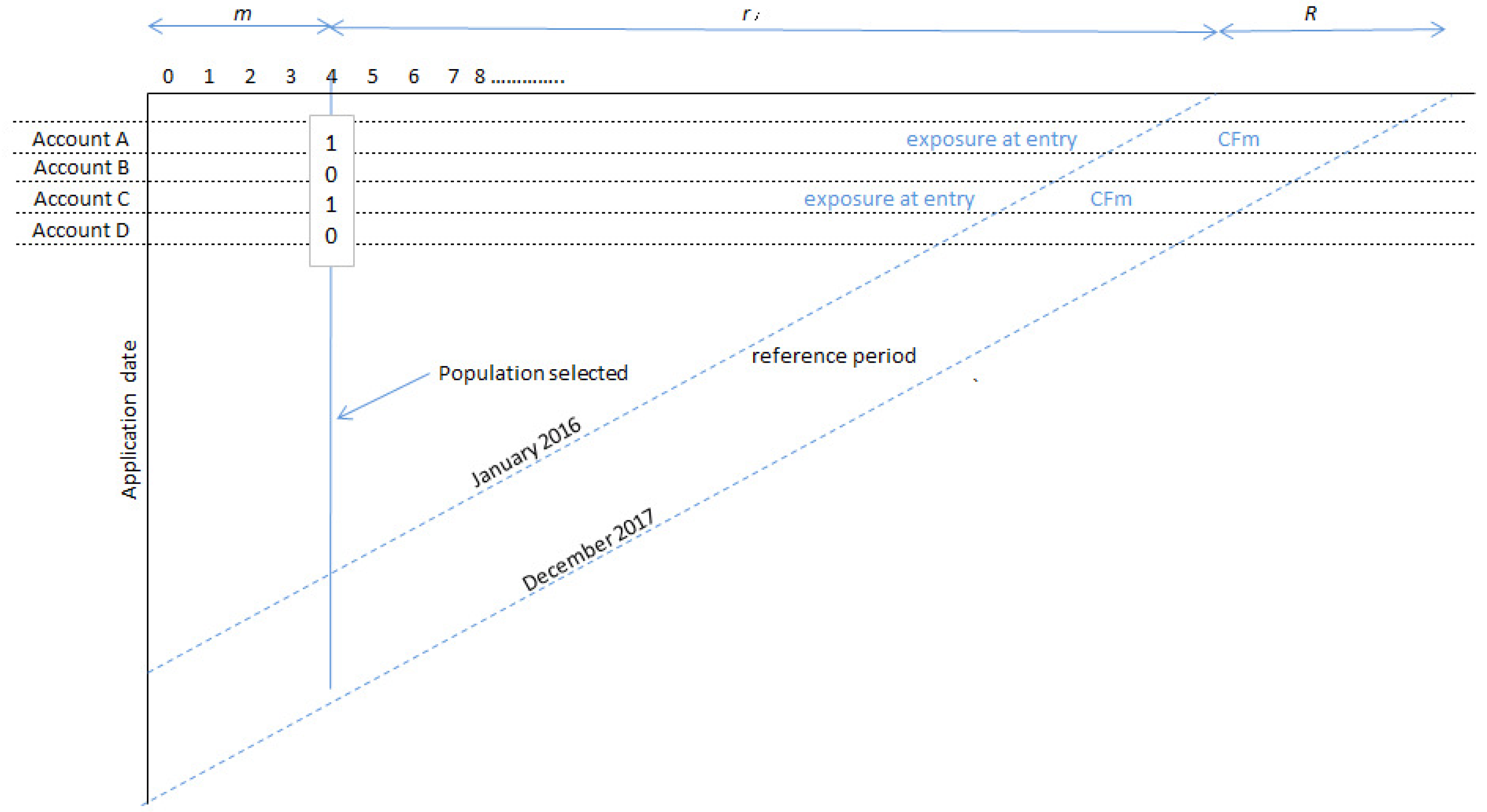
Figure 1. Definition of the reference period for IFRS 9 using an example.
Risks 09 00103 g001
Figure 2. Empirical IFRS 9 and Basel LGDs for the development period and out of time.
Risks 09 00103 g002
Figure 3. Empirical and estimated IFRS 9 LGD by month on book.
Risks 09 00103 g003
Figure 4. Comparison of the development and out of time LGD values.
Risks 09 00103 g004
Figure 5. Estimated vs the empirical IFRS 9 LGDs for the development and out of time reference period.
Risks 09 00103 g005
Figure 6. LGD by calendar month used as target in the ECM.
Risks 09 00103 g006
Figure 7. LGD by calendar month including forecasts for different scenarios.
Risks 09 00103 g007
Table 1. Test statistic values for the Augmented Dicky-Fuller test.
Macro-Economic
Variable
t-Value -
No Differencing
t-Value -
First Difference
t-Value -
Error
CPI−1.74−3.96−4.29
DDHI−2.23−5.84−5.78
debt affordability−1.26−5.75−6.58
DSR−1.22−5.44−3.97
GDP−2.97−4.24−5.86
leading indicator−0.44−4.45−5.48
liquidity spread−0.72−4.78−451
M3 money supply−0.71−4.74−4.85
NHPI−1.92−6.49−4.82
prime interest rate−1.87−5.26−5.36
rand dollar exchange rate−2.32−4.23−4.34
RHPI−0.93−5.39−5.51
Table 2. Results for the short-term portion of the ECM.
Parameter Estimates ϕ 0 = 0.32 ϕ 1 = 0.41 ϕ 2 = 0.51 ϕ 3 = 0.33
VariableInterceptGDPDDHIPrime
Lag used-Lag 3Lag 8Lag 7
VIF 2.441.022.42
Table 3. Results for the long-run portion of the ECM.
Parameter Estimates α 0 = 0 α 1 = 0.04 α 2 = 0.03
VariableInterceptLeading indicatorDebt affordability
Lag used-Lag 1Lag 5
VIF 1.371.59
Table 4. Macro-economic adjusted IFRS 9 LGD values.
Base
Scenario
Pessimistic
Scenario
Optimistic
Scenario
Probability of scenario occurring40%30%30%
% IFRS 9 LGD change from base-−4.03%5.17%
% IFRS 9 PD change from base-−2.07%3.29%
% ECL change from base-−3.27%4.39%
Publisher’s Note: MDPI stays neutral with regard to jurisdictional claims in published maps and institutional affiliations.