Empirical Evidences on the Interconnectedness between Sampling and Asset Returns’ Distributions

Abstract

The aim of this work was to test how returns are distributed across multiple asset classes, markets and sampling frequency. We examine returns of swaps, equity and bond indices as well as the rescaling by their volatilities over different horizons (since inception to Q2-2020). Contrarily to some literature, we find that the realized distributions of logarithmic returns, scaled or not by the standard deviations, are skewed and that they may be better fitted by t-skew distributions. Our finding holds true across asset classes, maturity and developed and developing markets. This may explain why models based on dynamic conditional score (DCS) have superior performance when the underlying distribution belongs to the t-skew family. Finally, we show how sampling and distribution of returns are strictly connected. This is of great importance as, for example, extrapolating yearly scenarios from daily performances may prove not to be correct.

1. Introduction

The aim of this article was to investigate the interconnectedness between sampling and asset returns’ distributions. To this end, we empirically perform a number of analyses across asset classes, markets and for several sampling frequencies. The topic is quite relevant as both vendors and financial institutions may rely on scenarios generated under the assumption that financial series returns are normally distributed. There are some works which claim that standardized daily returns “are approximately unconditionally normally distributed” Andersen et al. (2001) or that “are IID Gaussian, with variance equal to 1” Rogers (2018).

A more realistic work hypothesis is that time series follow a t-skew distribution. The t-skew distribution can be seen as a mixture of skew-normal distributions Kim (2001) which generalize the normal distribution thanks to an extra parameter regulating the skewness. By construction, then, they can model heavy tails and skews that are common in financial markets. Thus, their adoption in finance is gaining momentum for modeling distributions Harvey (2013) and risk Gao and Zhou (2016). Further, t-skew has the power to link-up with observation-driven models such as the dynamic conditional score (DCS) Creal et al. (2013) or based on data partitioning Orlando et al. (2019, 2020). This paper tries to help in gaining insights on returns’ distributions and on the most suitable way of fitting them.

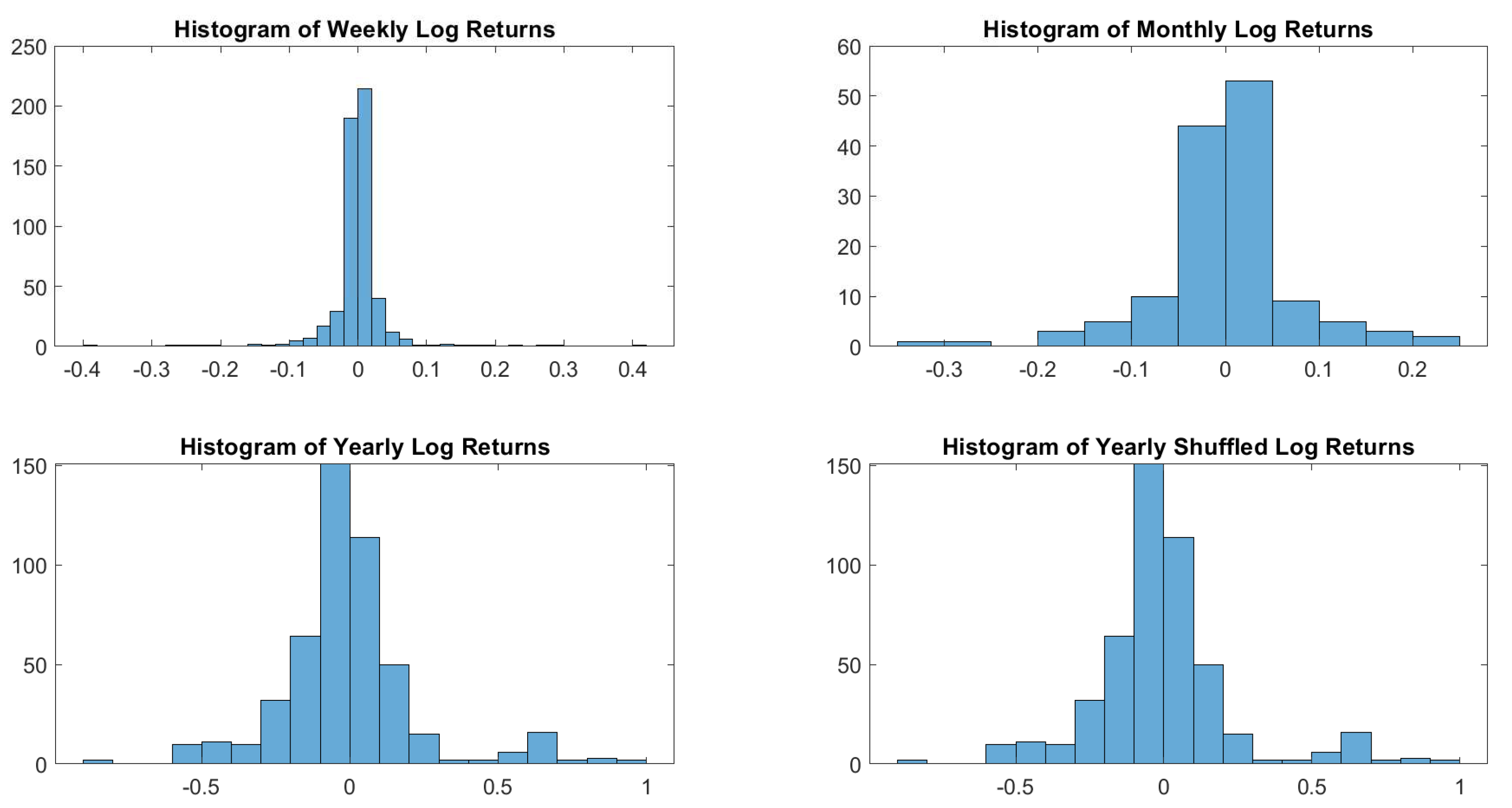
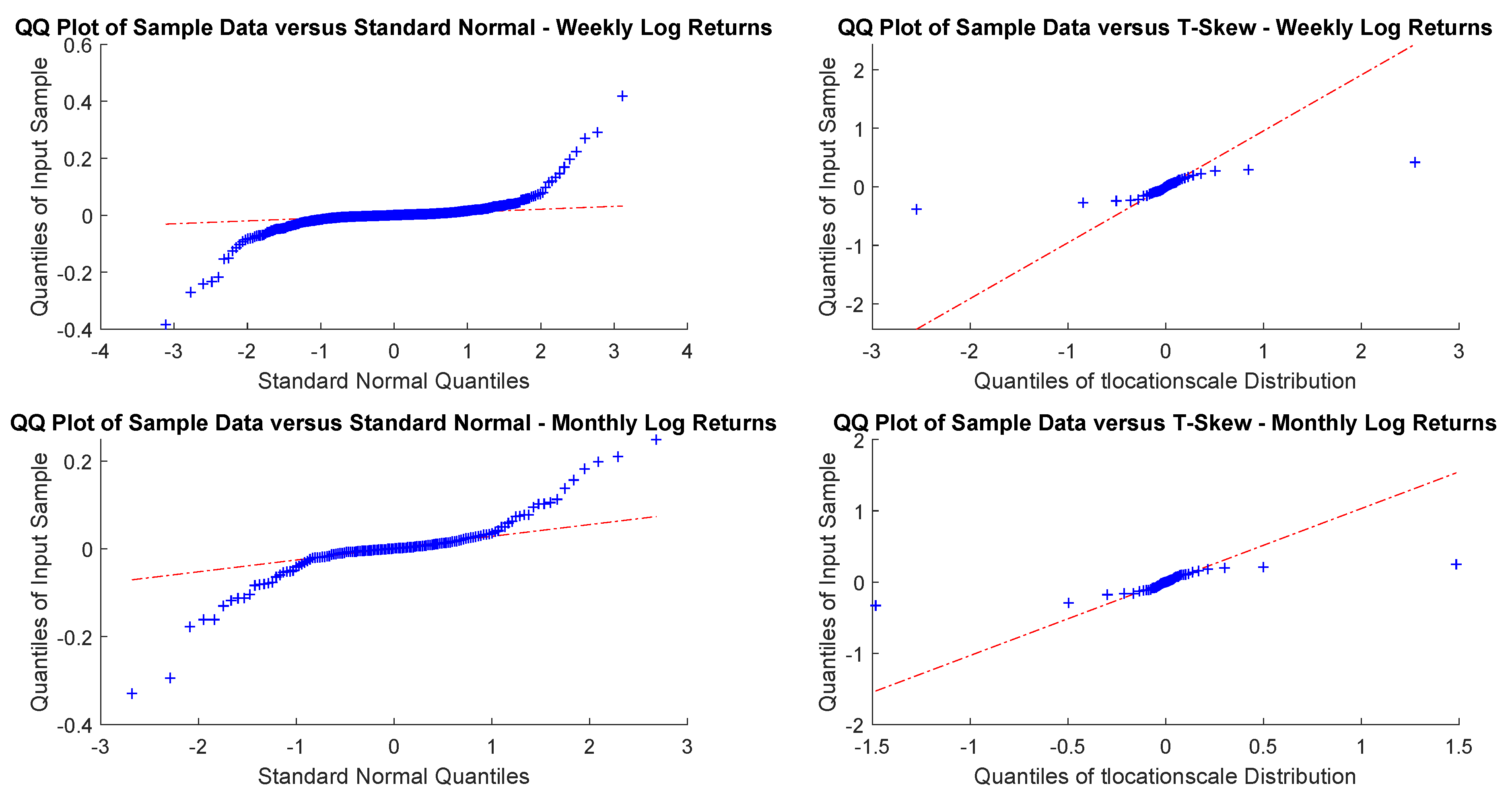
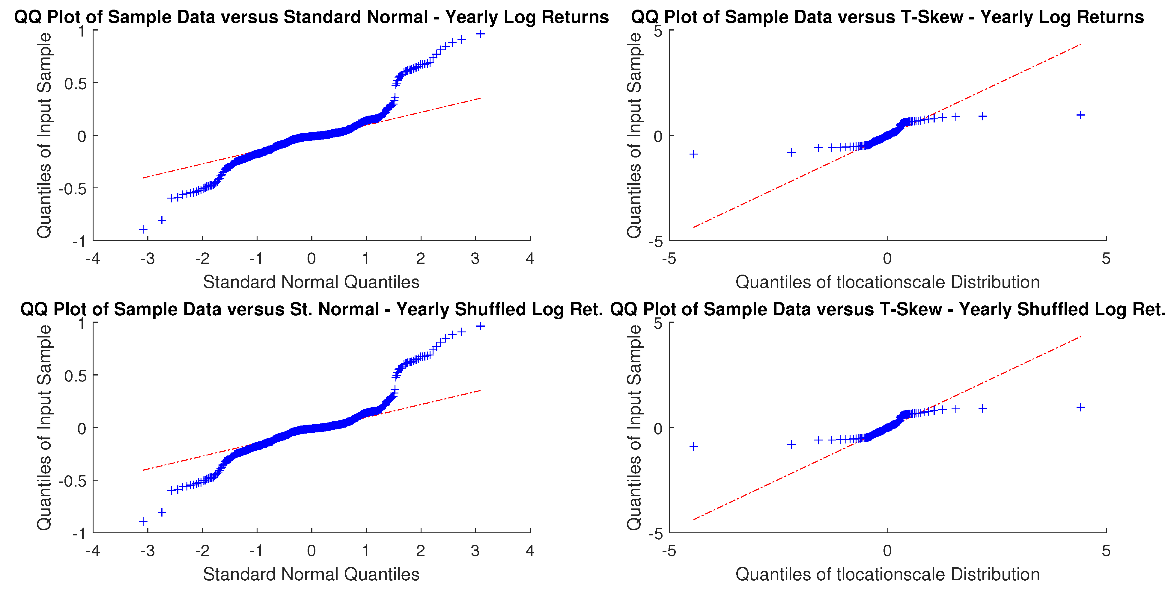
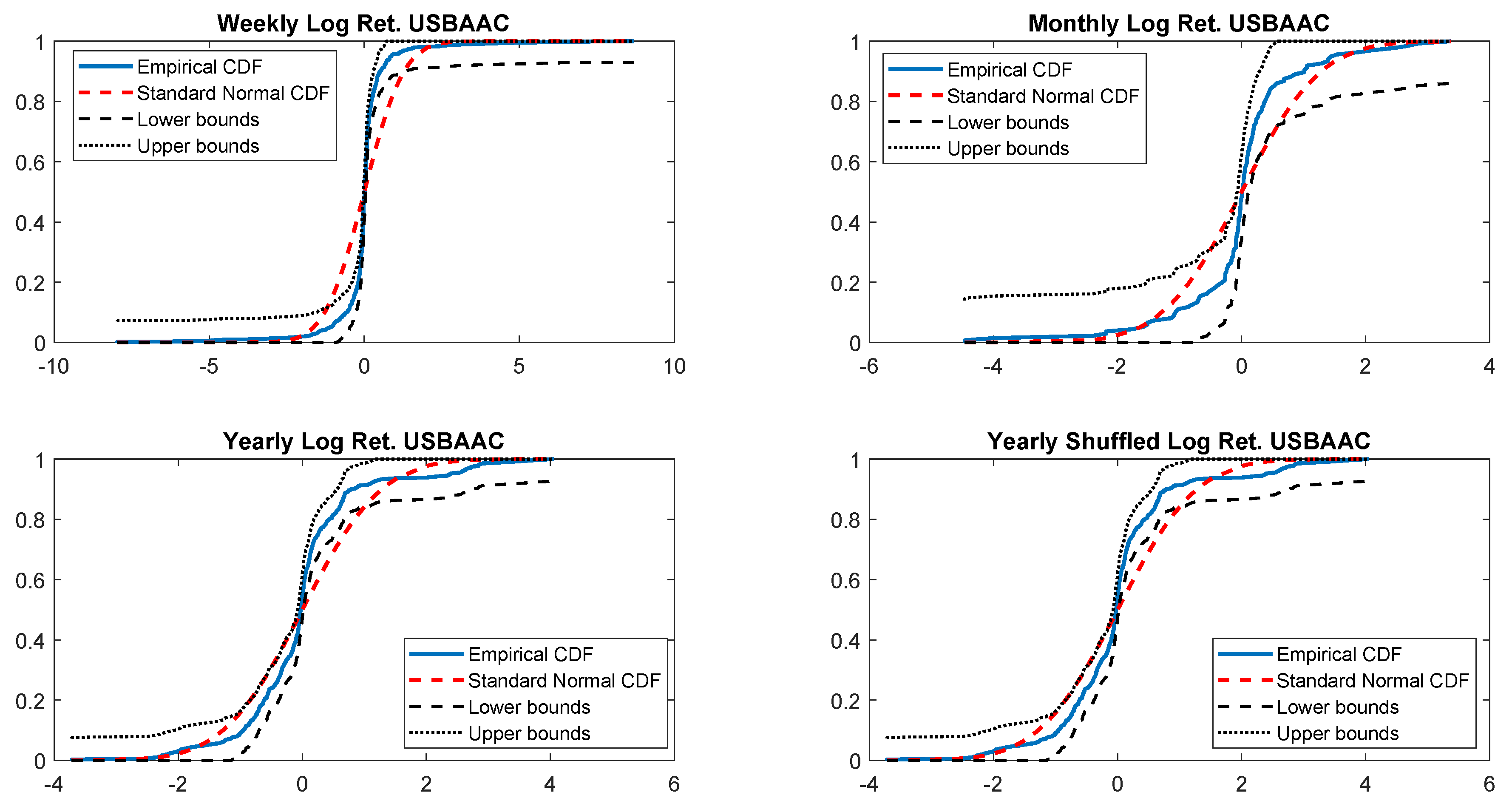
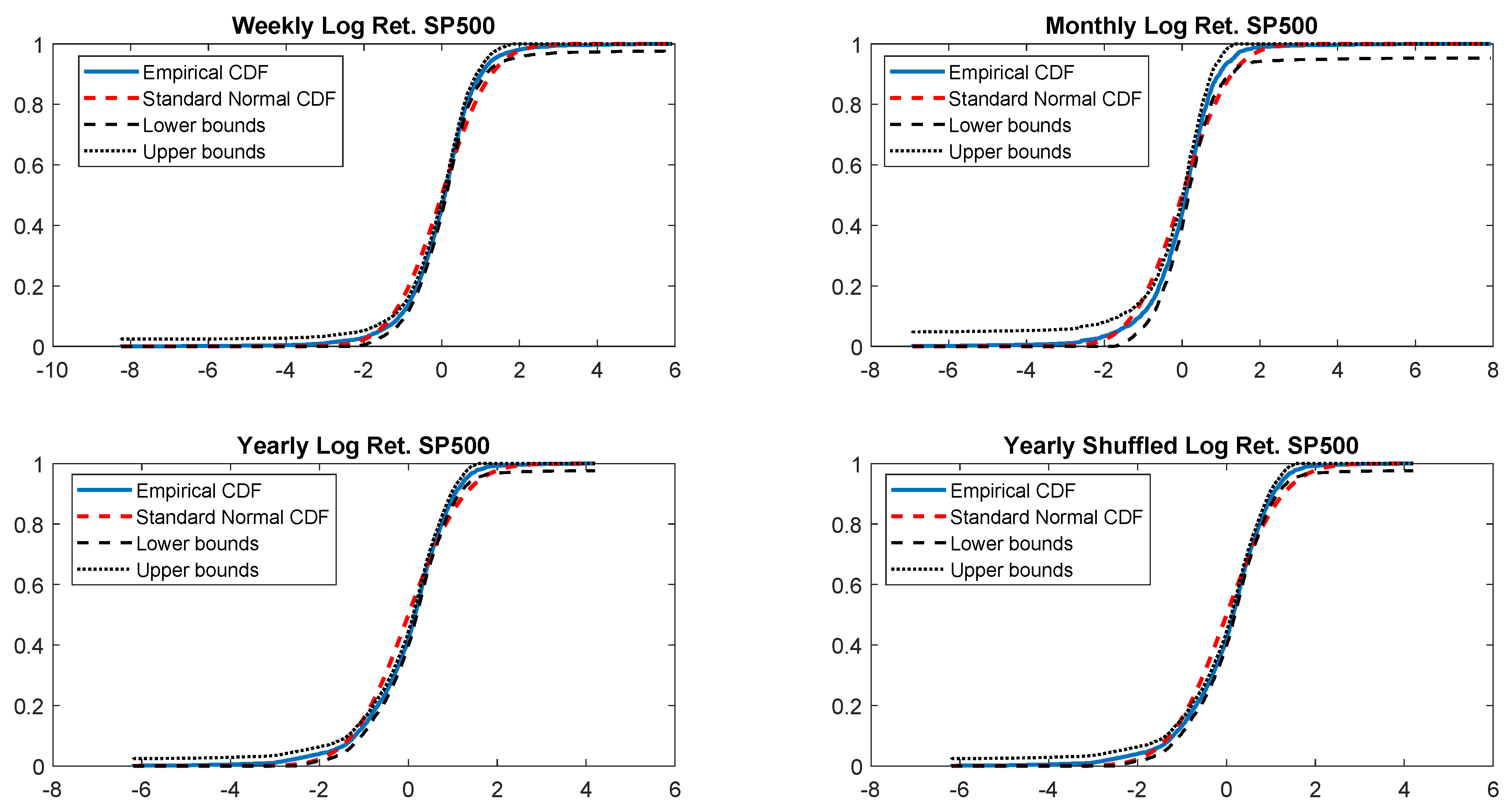
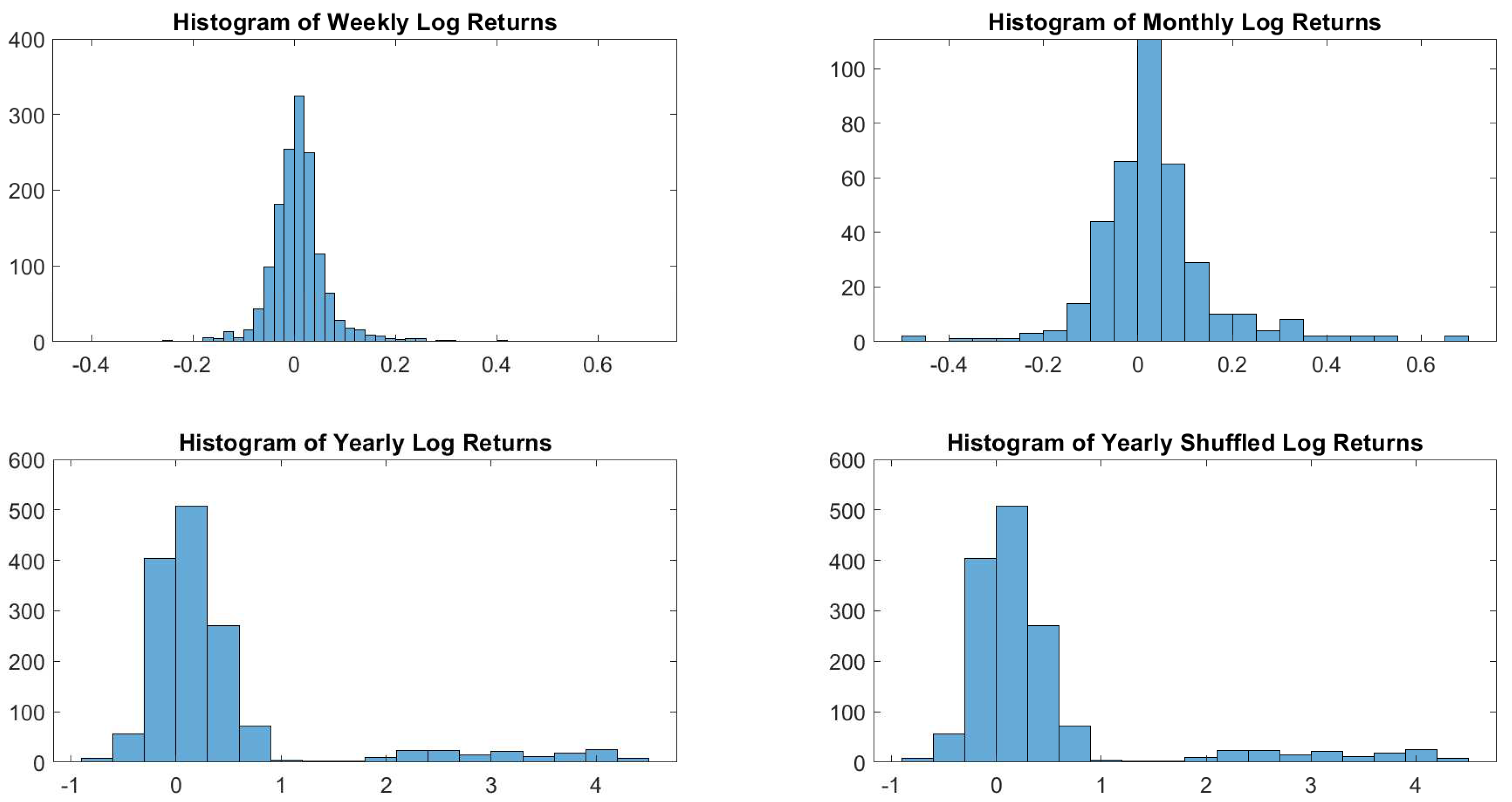
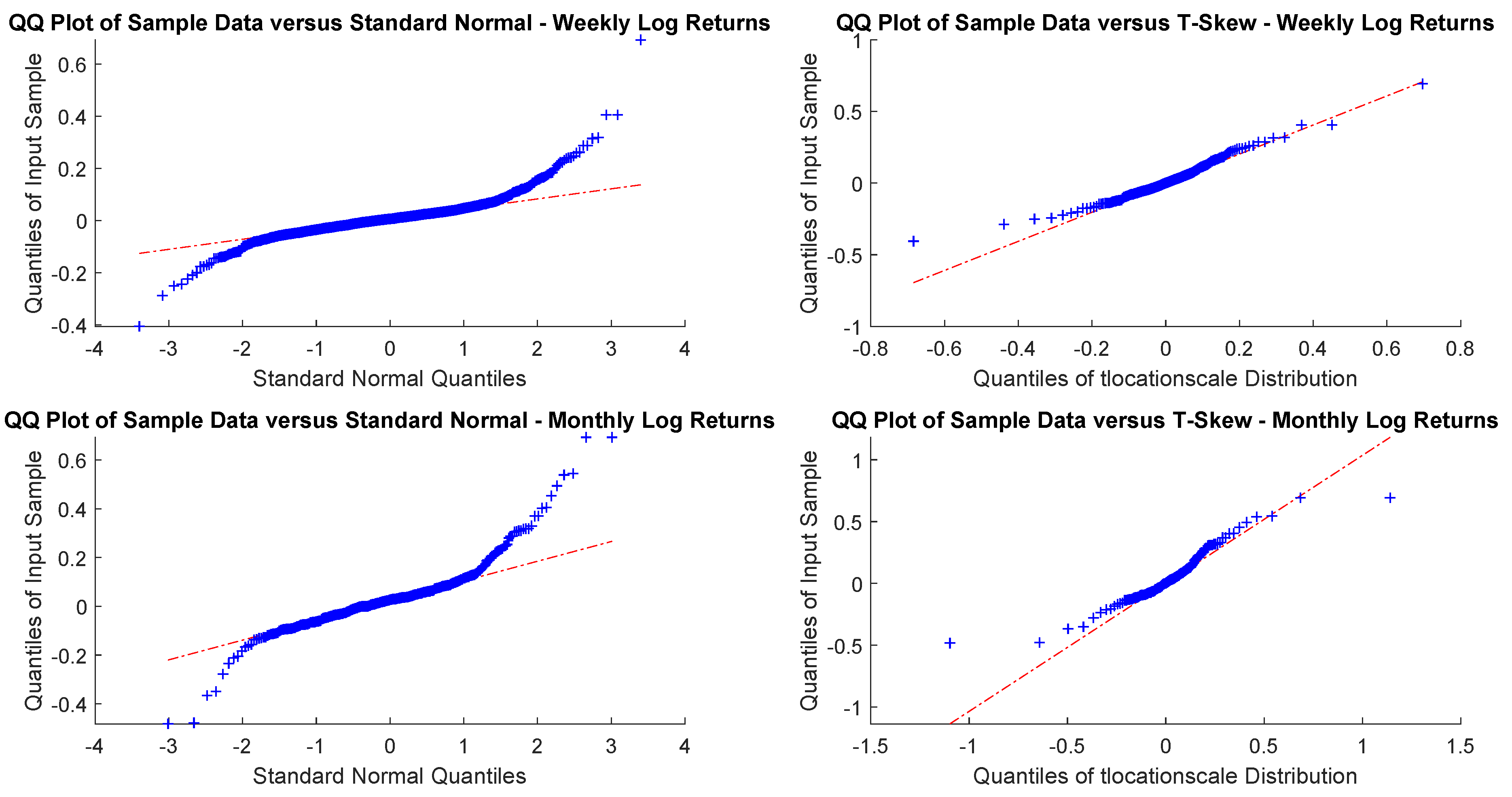
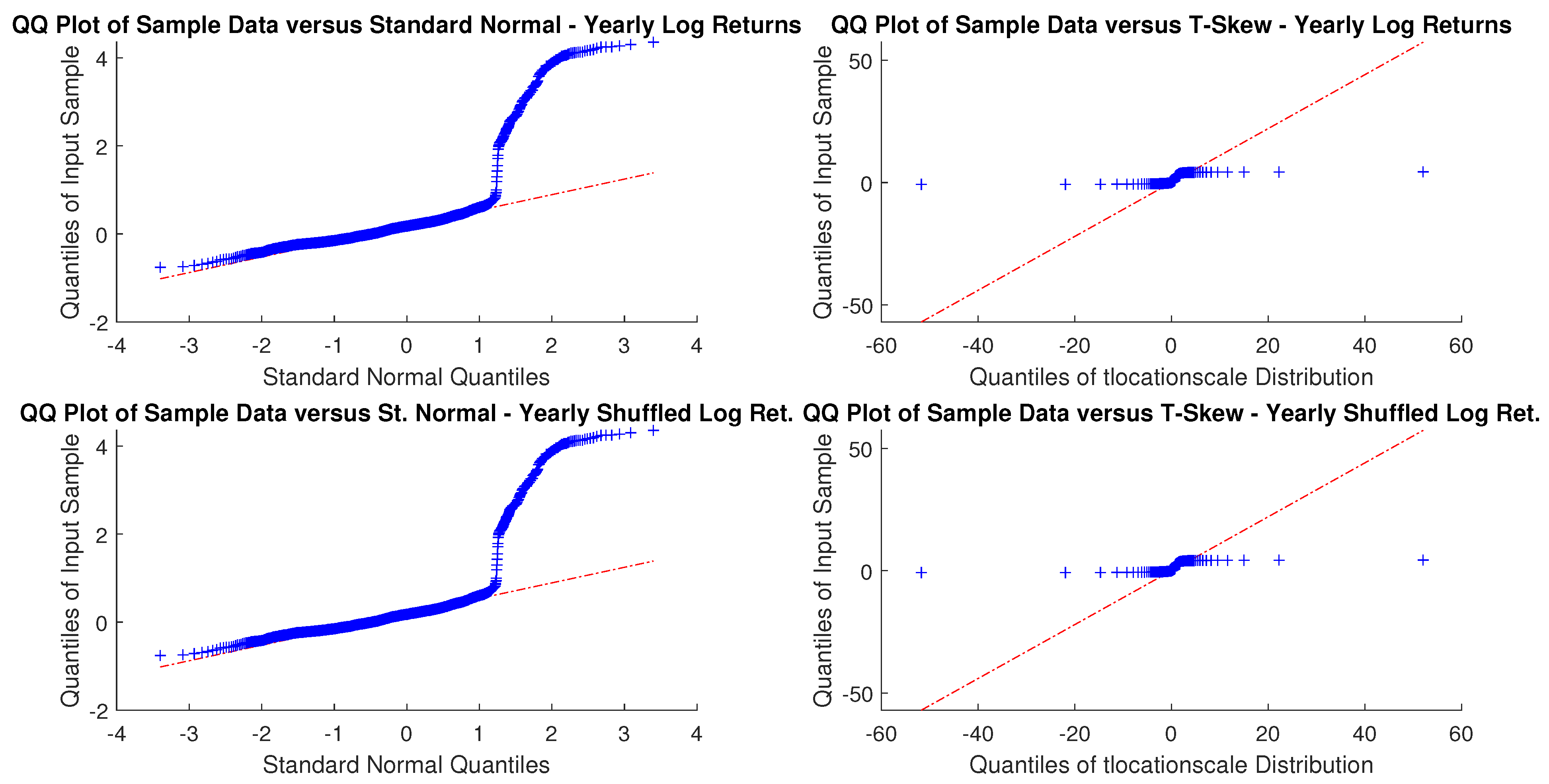
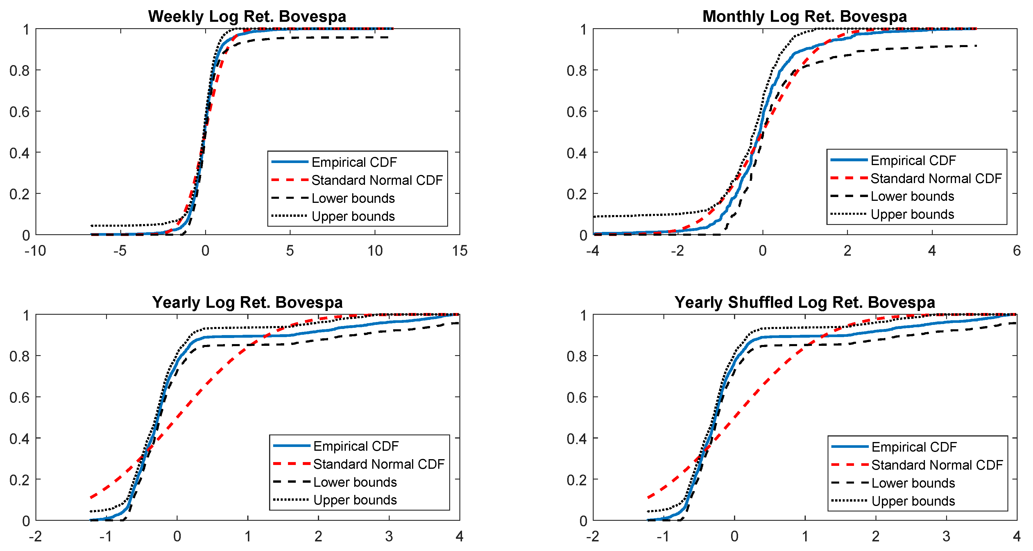
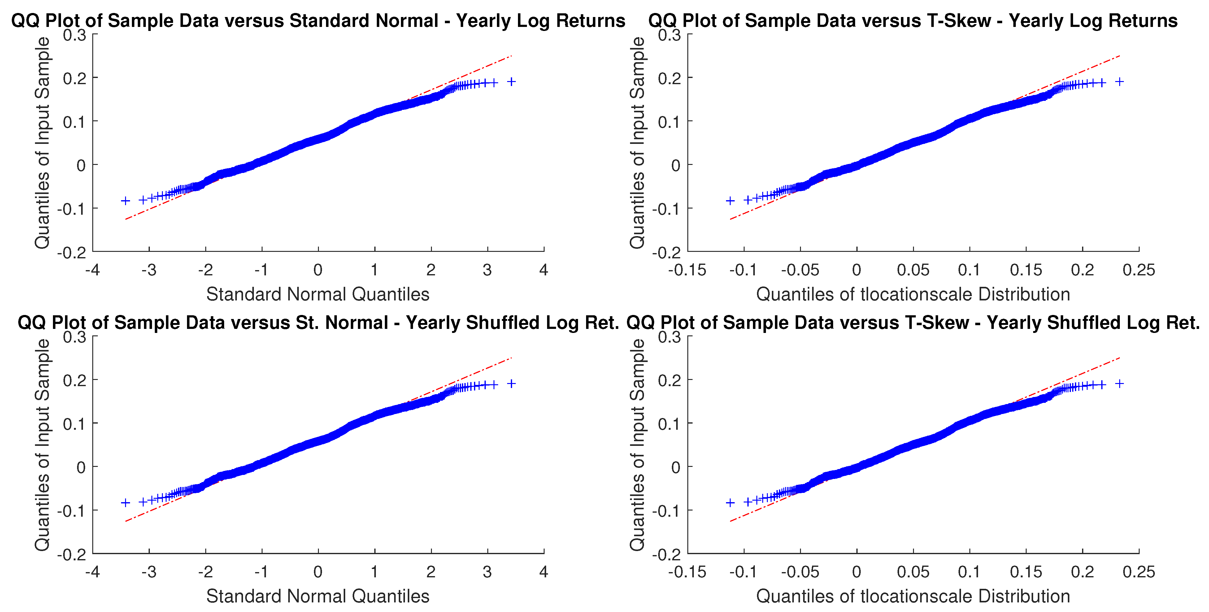
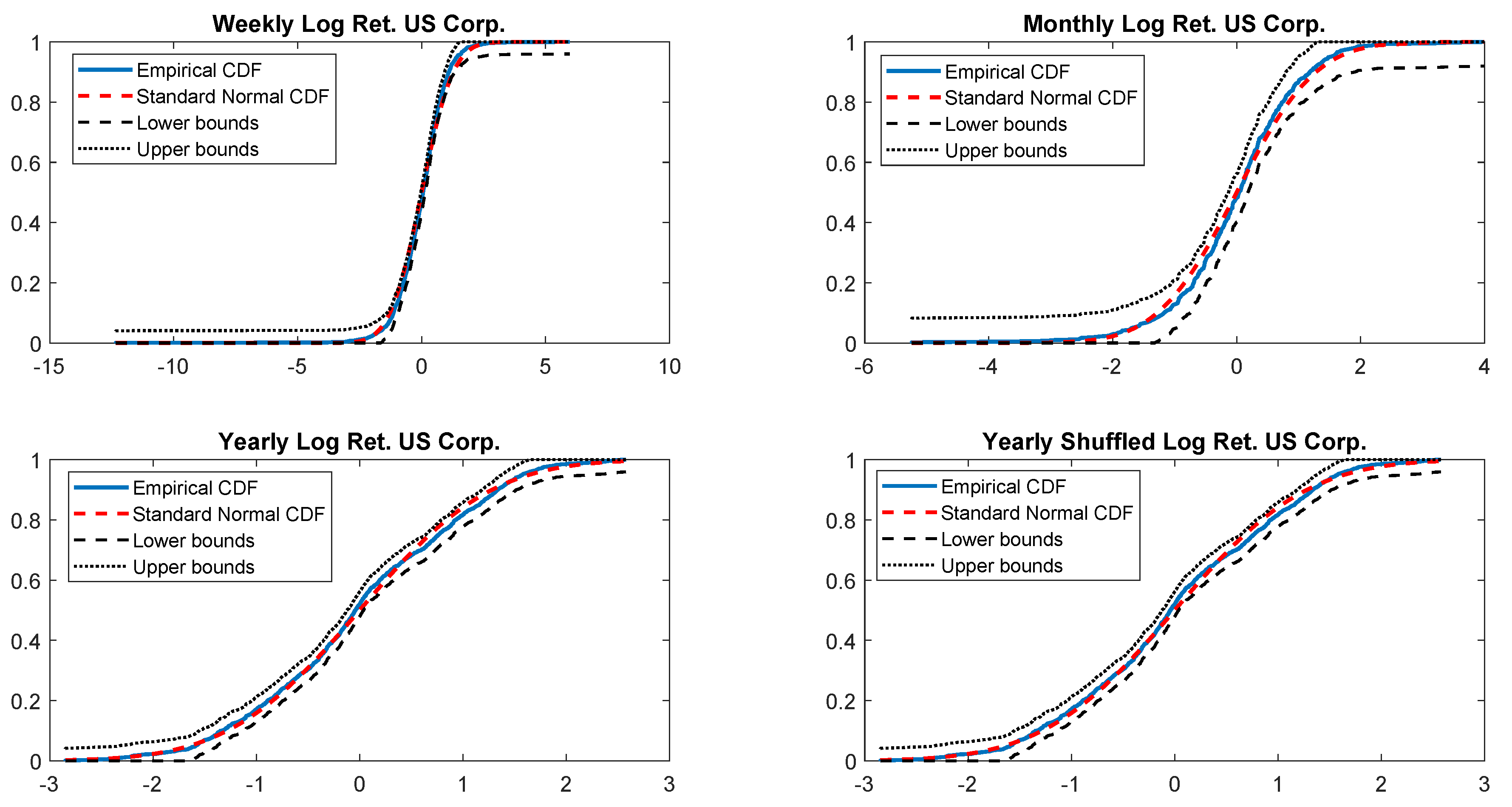
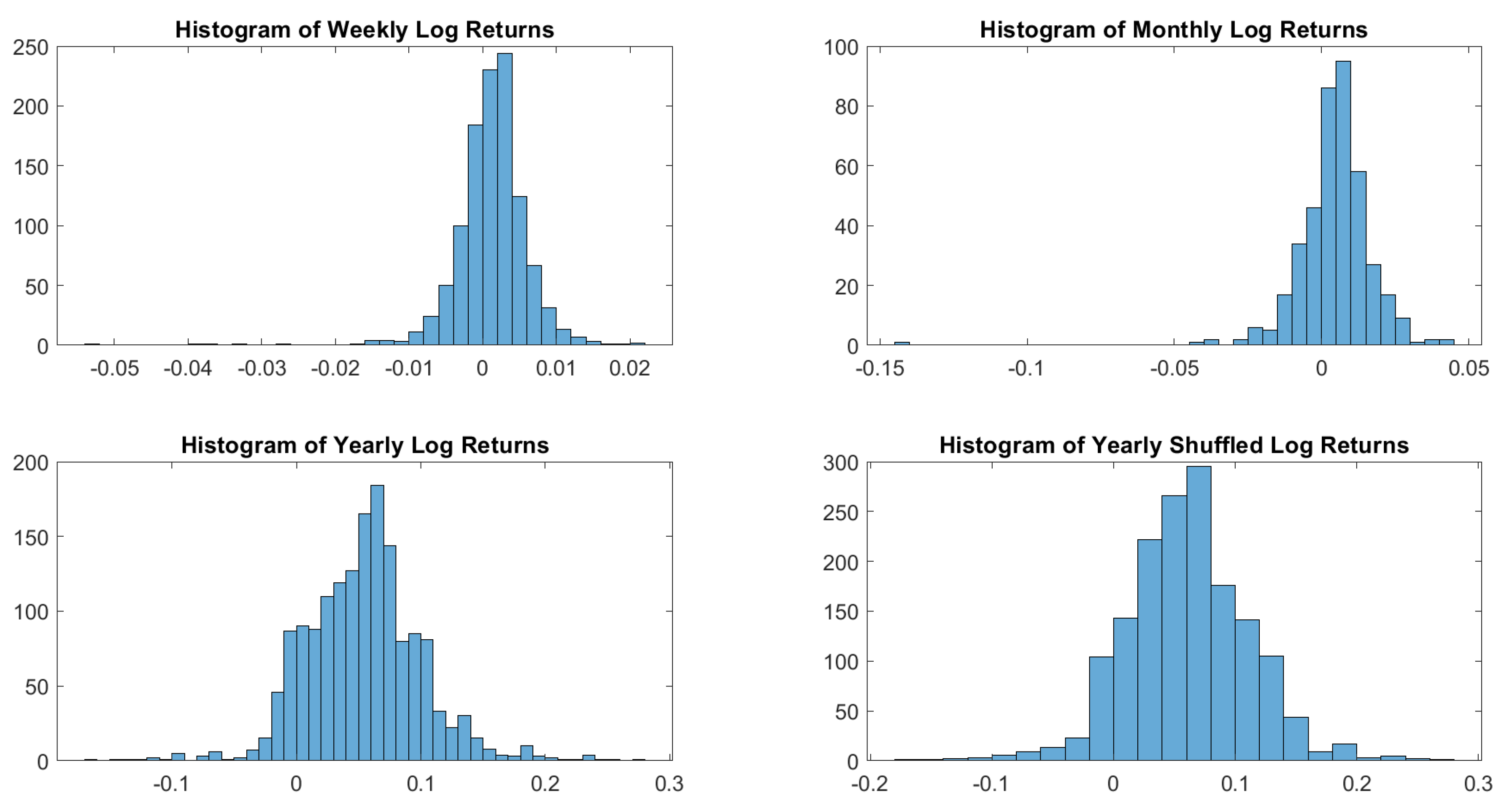
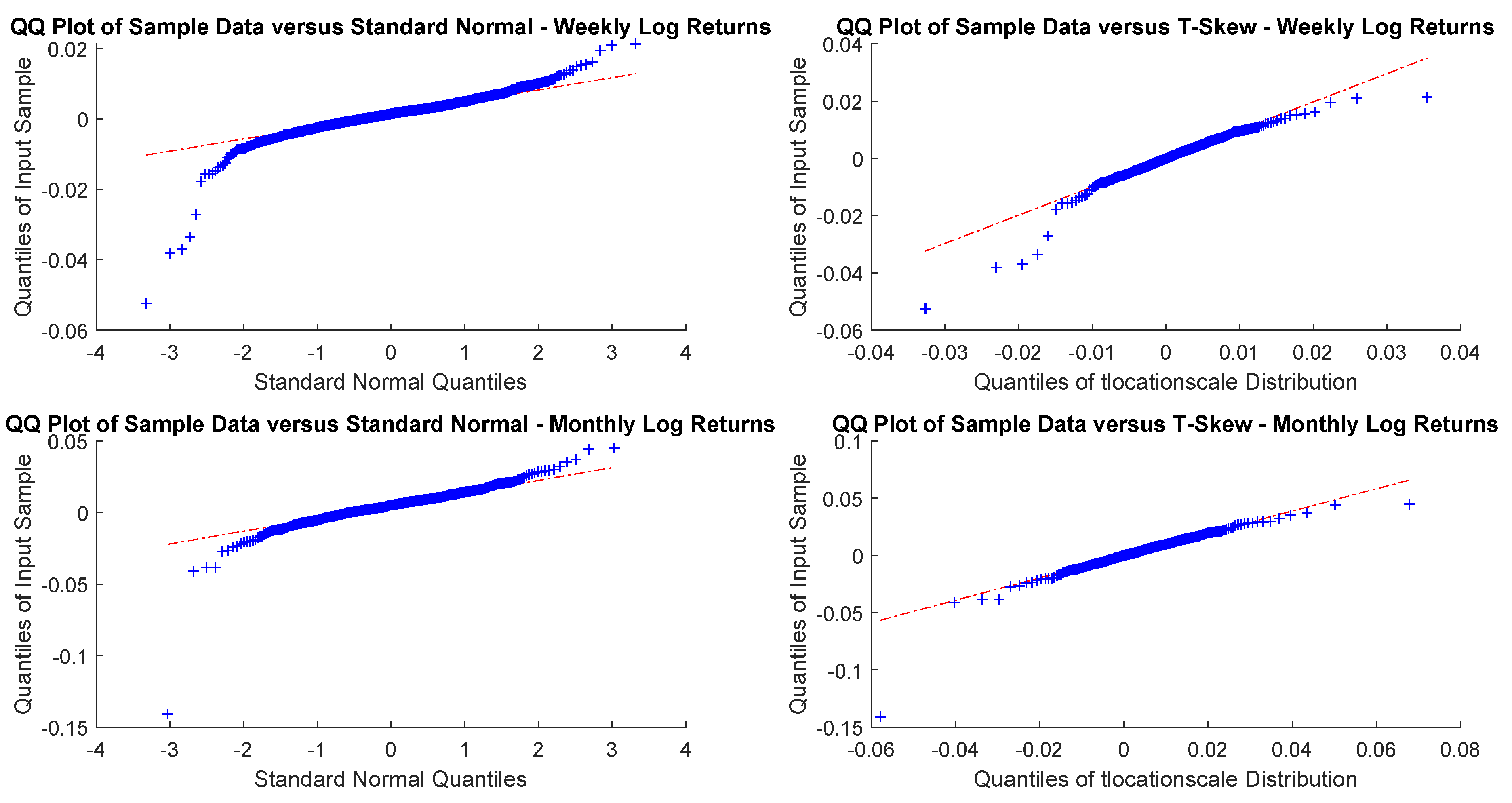
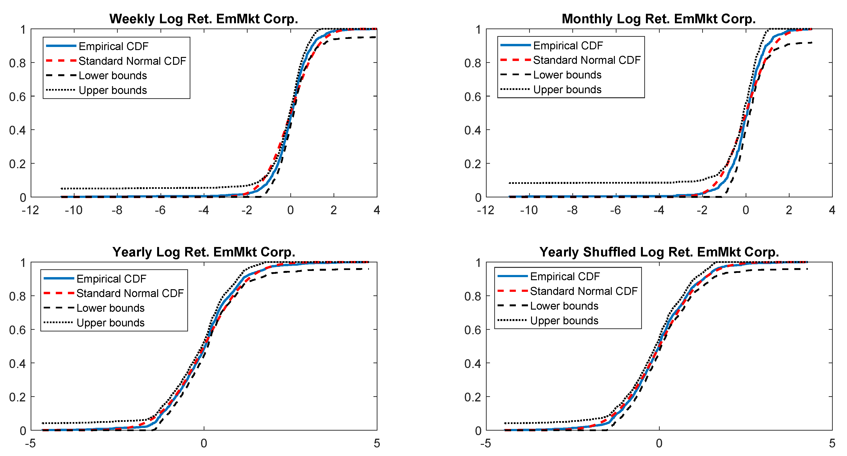
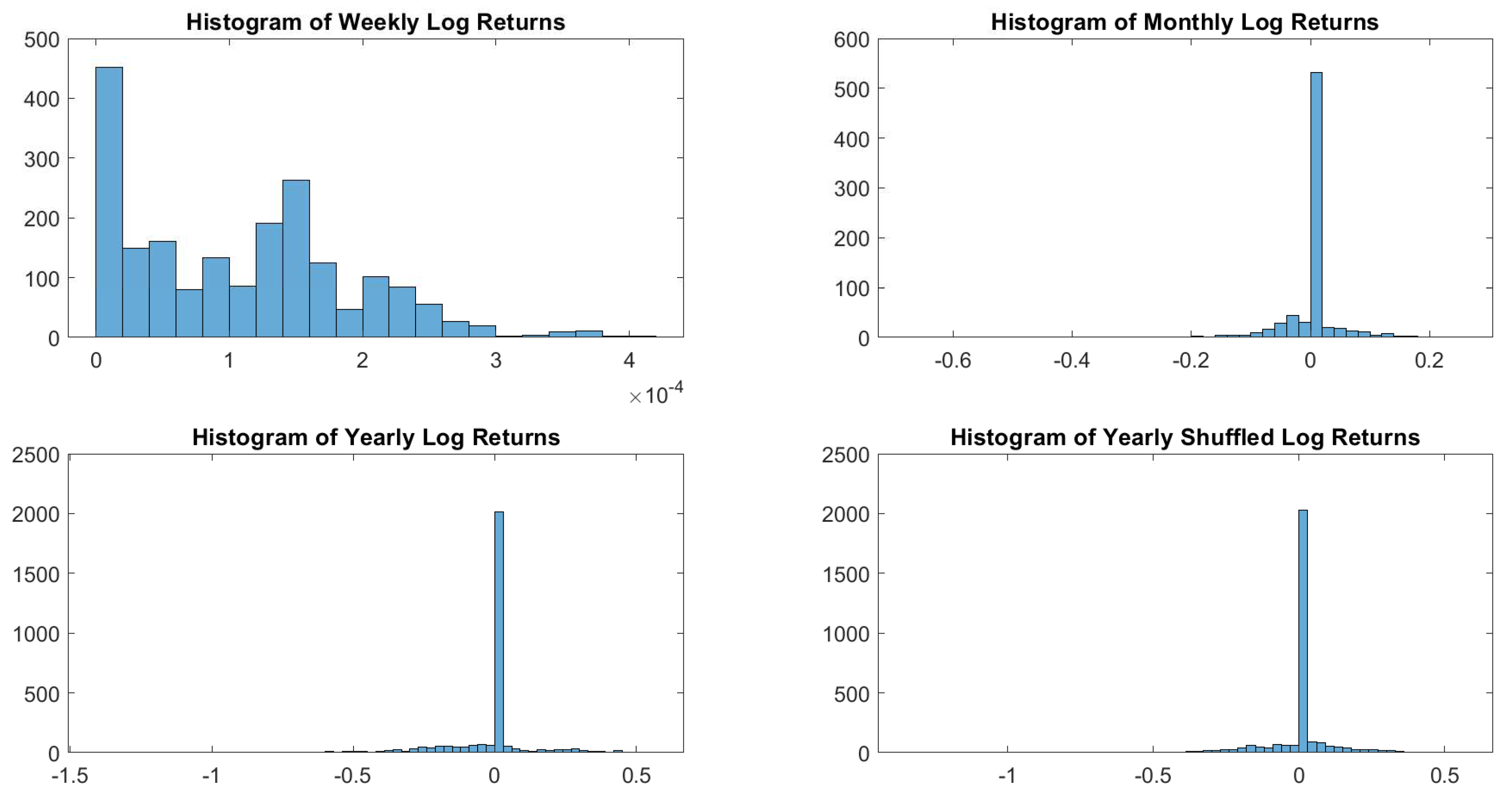
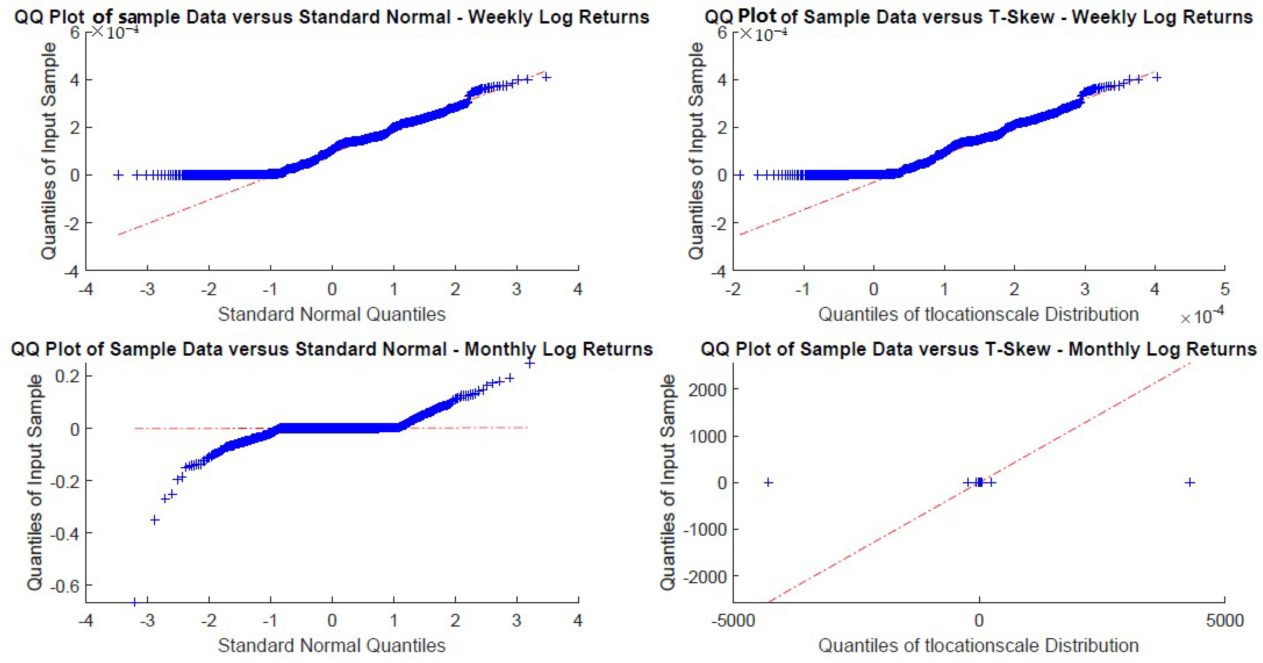
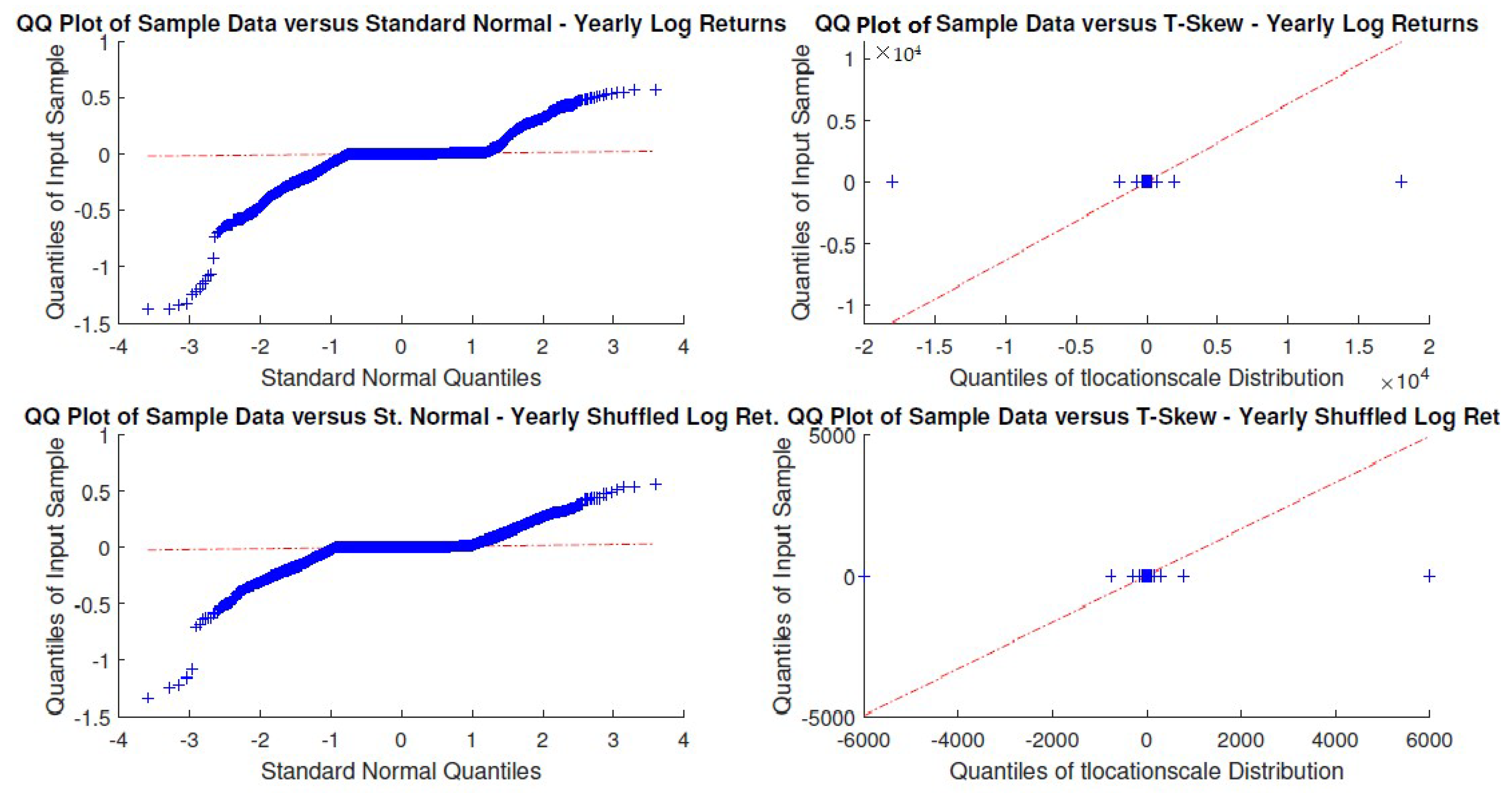
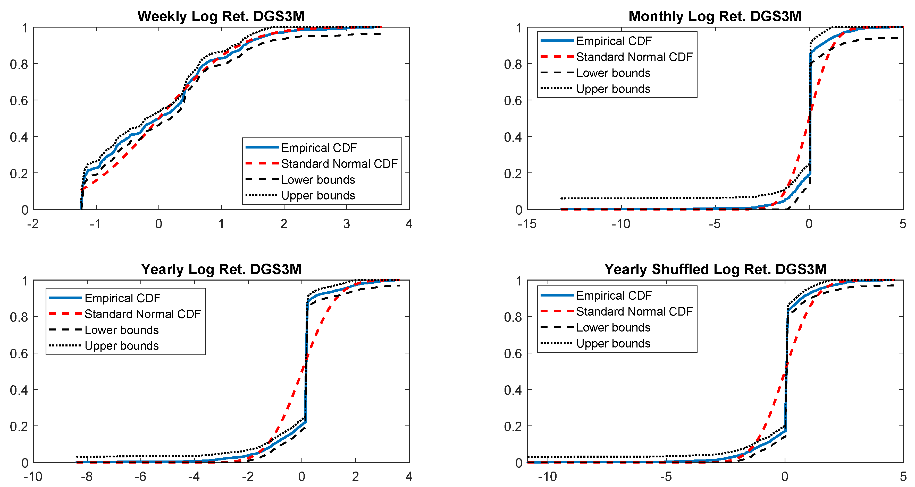
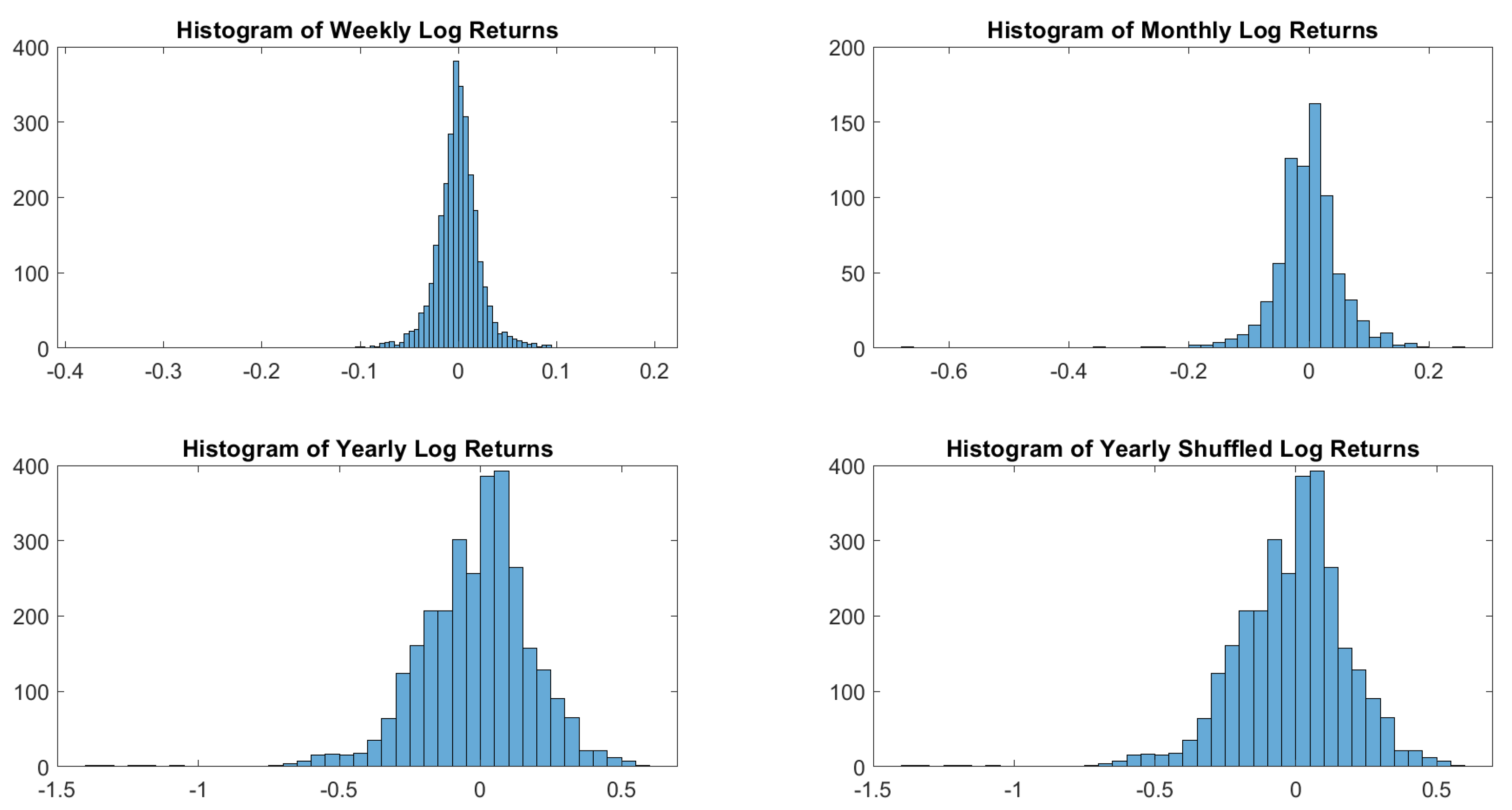
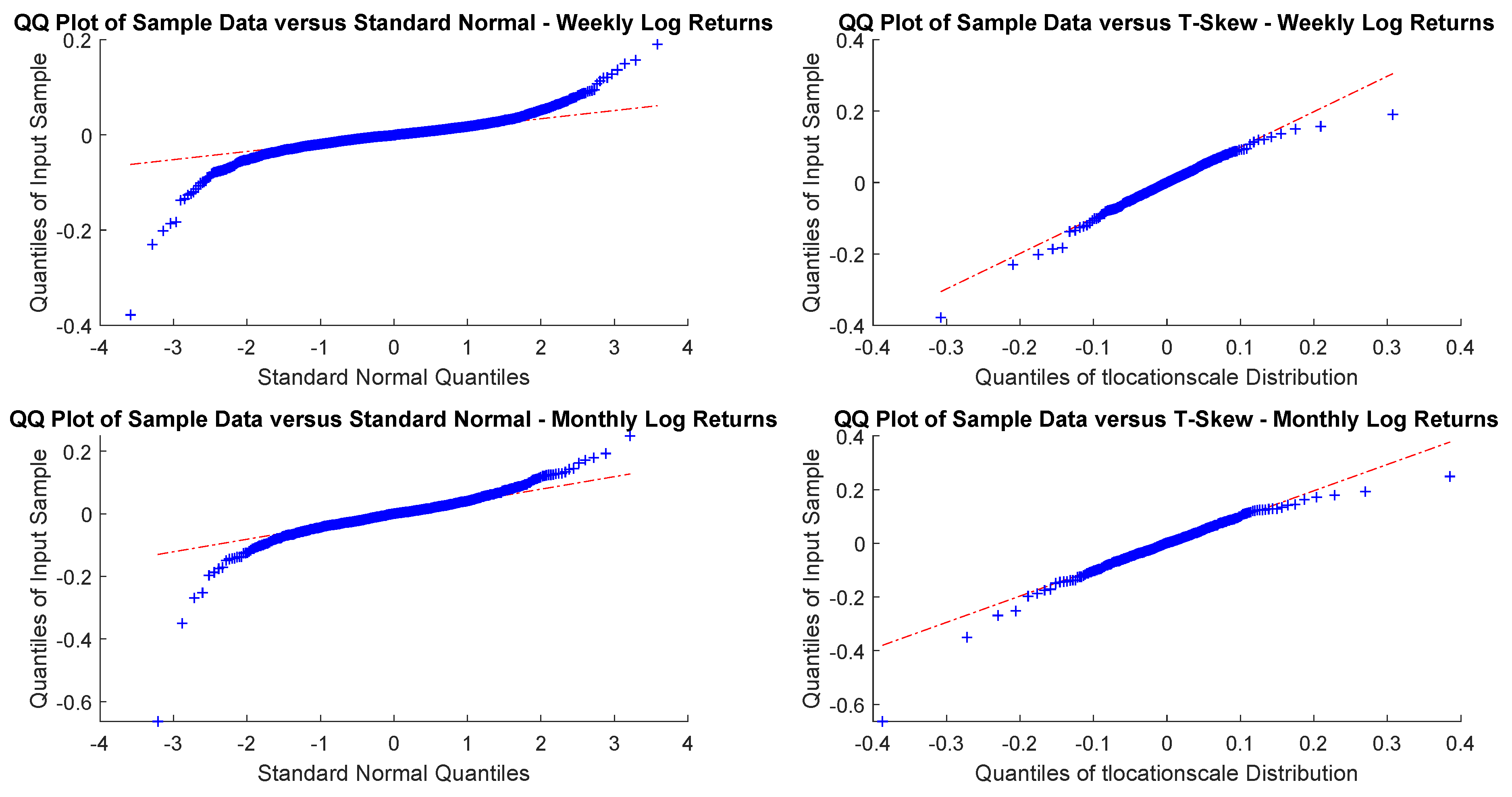
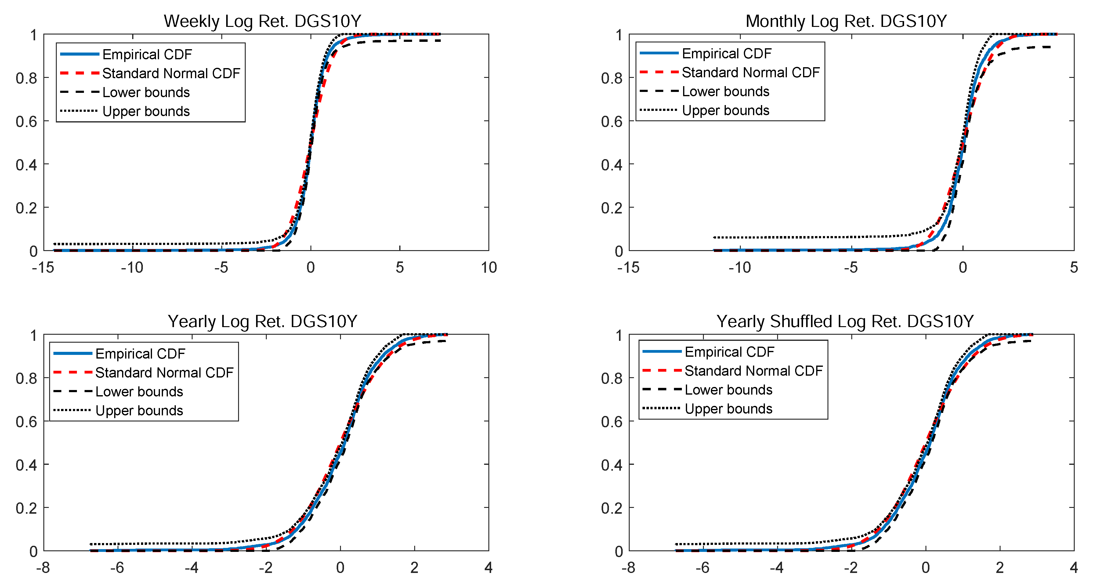
In particular, according to the tests carried out on our dataset, the distributions of log-returns do not seem to be normally distributed. The same applies on the returns standardized by the standard deviation. In a different context, Tiwari and Gupta (2019) found that the Jarque–Bera test strongly rejects the hypothesis of Gaussian distribution for all considered time series concerning G7 stock markets. Therefore, through the paper, we report a number of tests to decide the better distribution between Gaussian, t-skew, generalized hyperbolic, generalized Pareto and exponential Pareto. In terms of applications, being able to correctly identify the distribution is important for risk management as the tail conditional expectation provides information about the mean of the tail of the loss distribution, “while the tail variance (TV) measures the deviation of the loss from this mean along the tail of the distribution” Eini and Khaloozadeh (2020). Another application is in option pricing. For instance, Yeap et al. (2018) propose a t-skew model with “a fat-tailed, skewed distribution and infinite-activity (pure jump) stock dynamics, which is achieved through modeling the length of time intervals as stochastic”.

Having described the framework of our investigation, now we are in position to perform some tests on swaps, equities (for both developed and emerging markets) and corporate bonds (for both developed and emerging markets) sampled on weekly, monthly and yearly basis. Section 2 contains a literature review, Section 3 describes the dataset and the methods we intend to adopt for our analysis, Section 4 reports the results we obtained on the original data as well as on the time series of the rescaled returns, the last Section 5 draws the conclusions.

2. Literature Review

Distribution of returns is important because econometric models depend upon specific distributional assumptions, and in the case of implied volatilities, on further assumptions concerning the distributional and dynamic properties of stock market volatility. Wrong assumptions call into question the robustness of findings based on those models. One may always opt for an alternative approaches such as those based on squared returns over a given horizon, that provides model-free unbiased estimates of the ex-post realized volatility. Unfortunately, however, “squared returns are also a very noisy volatility indicator and hence do not allow for reliable inference regarding the true underlying latent volatility” Andersen et al. (2001). To overcome such limitations, Andersen et al. 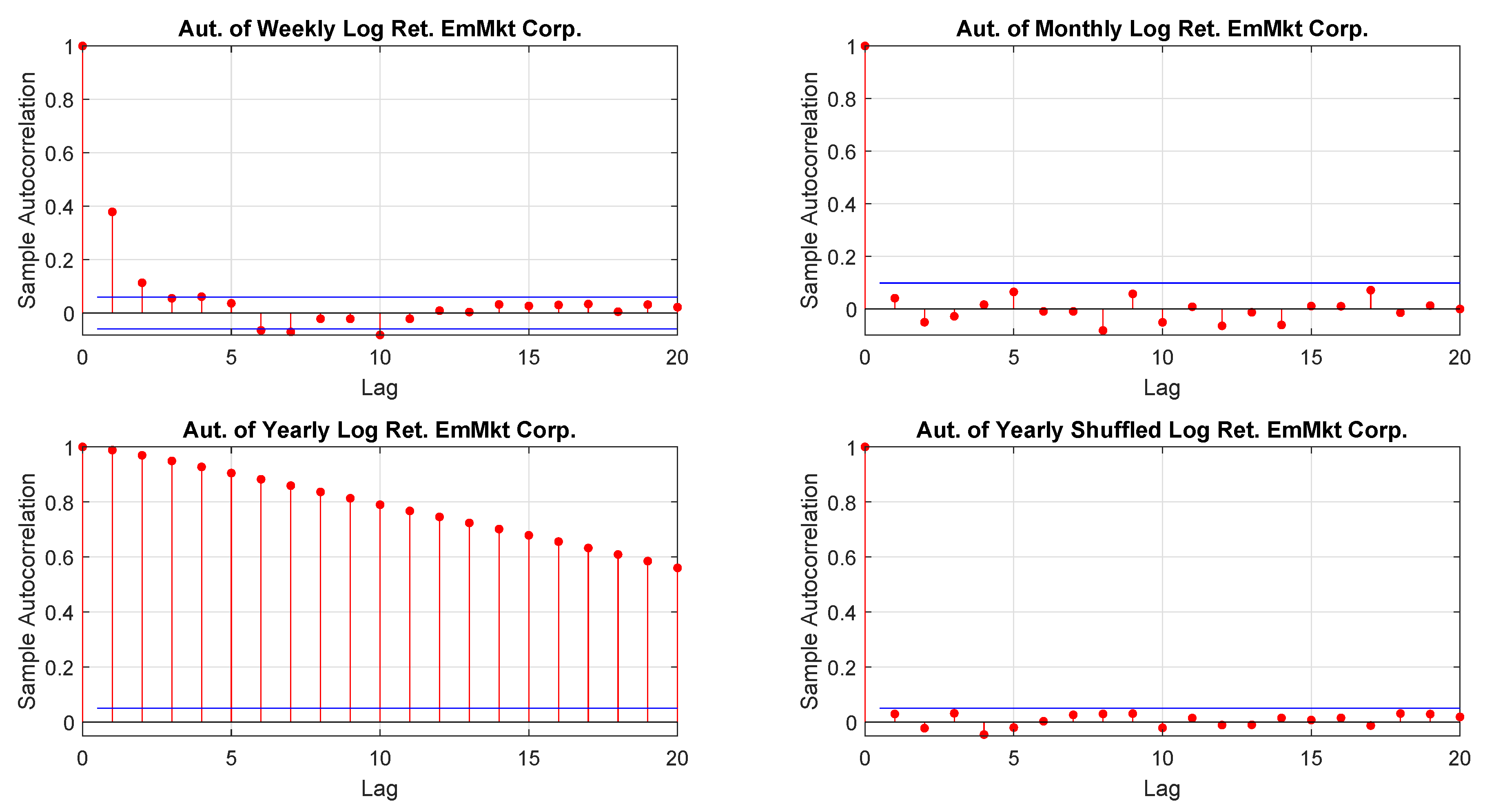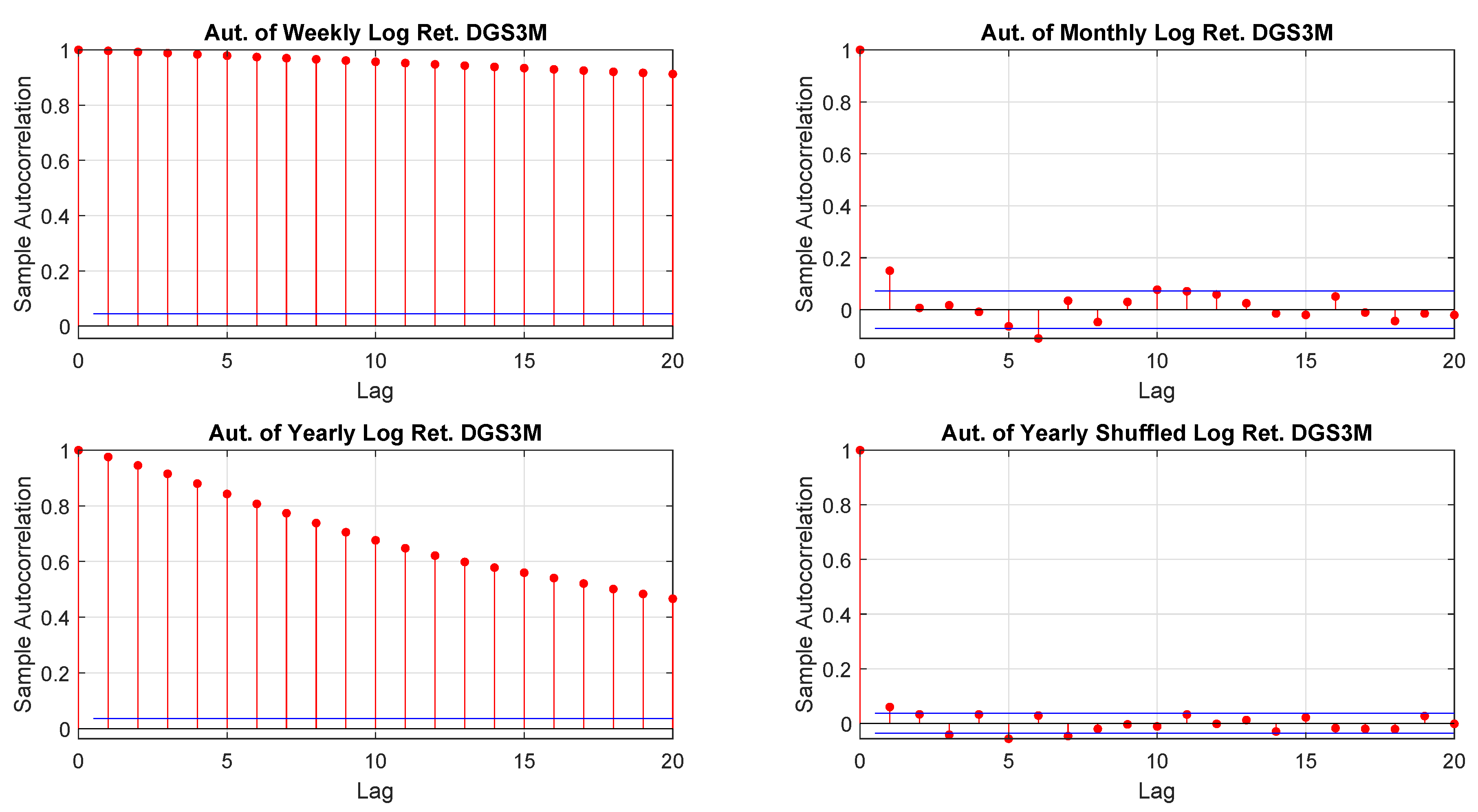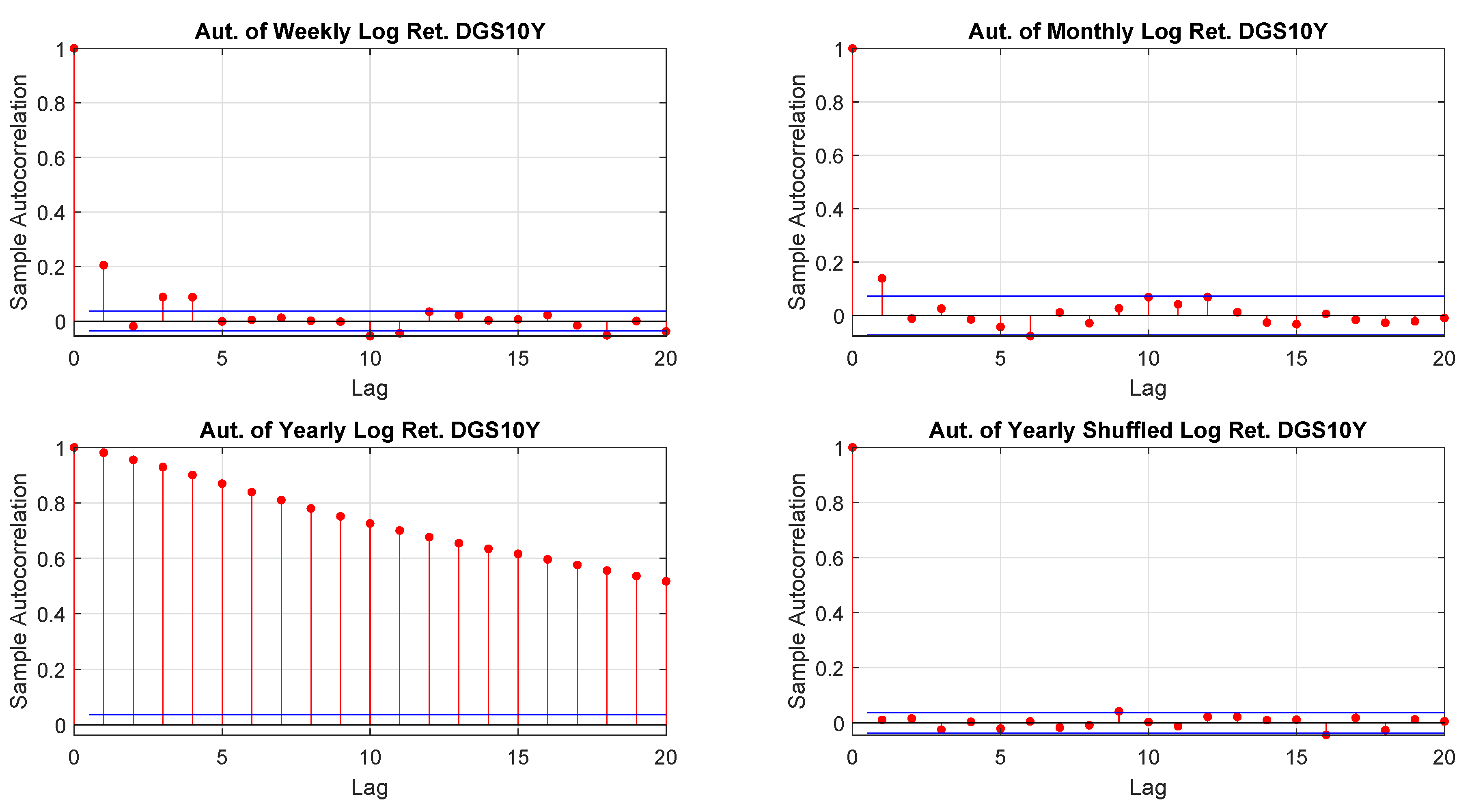(2001) suggested a model free volatility estimate by summing squares and cross-products of intraday high-frequency returns. That approach, however, relies on a reliable high-frequency return observation which, often is not guaranteed. Moreover, it is not necessarily true that the characteristics of a time series are independent on the time horizon and the sampling frequency so that, for example, one may extrapolate seeminglessly from daily data monthly or yearly distributions. Furthermore, time horizon and sampling frequency not only may influence the moments of a given distribution of returns but, also, the way in which data are hierarchically and spatially organized Tumminello et al. (2007).

According to McNeil et al. (2015), a bivariate t-Student distribution can describe a pair of daily stock returns. In fact, multivariate stock returns could be modeled by the means of a t-Student copula Aas et al. (2009) and Nikoloulopoulos et al. (2012). However, t-Student imposes symmetric dependence on the joint upper and lower tails which contrasts with empirical studies, e.g., Ang and Chen (2002); Longin and Solnik (2001); Patton (2006).

Among alternatives, parametric approaches skew normal distributions, as introduced by Azzalini (1985) and Henze (1986), have became quite popular because they suit well in modeling skewed data defined as follows

$$f(z;\theta )=2\phi \left(z\right)\Phi \left(z\theta \right)\hspace{1em}\hspace{1em}\hspace{1em}z\in \mathbb{R},$$

(1)

where $\theta$ is the parameter controlling the skewness and $\phi$ and $\Phi$ denote the $N(0,1)$ are the standard normal density and the normal cumulative distribution, respectively.

By further enhancing those distributions, Kim (2001) proposes a family of t-skew distributions in terms of a scale mixture of skew-normal distributions.

The random variable X is said to be t-skew distributed with parameter $\theta$ and $\nu$ if its probability density function is

$$f(x;\theta ,\nu )=2\mathbb{E}[z^{1/2}\phi \left(z^{1/2}x\right)\Phi \left(z^{1/2}\theta x\right)|z]\hspace{1em}\hspace{1em}\hspace{1em}x\in \mathbb{R},$$

(2)

where $z\sim \Gamma (\nu /2,2/\nu )$, $\phi$ and $\Phi$ are the standard normal density and the normal cumulative distribution, respectively.

The salient features of the family of t-skew distributions are their mathematical tractability, the inclusion of the normal law and the shape parameter regulating the skewness, apart from the ability of fitting heavy-tailed and skewed data, scale mixtures of skew-normal densities come from a family of t-skew distributions.

Such an extension allows for a continuous variation from normality to non-normality and it has found a number of applications on fitting heavy-tailed and skewed data. Other applications of such distributions are related to copula modeling. Yoshiba (2018) found that the AC t-skew copula describes well the dependence structures of both “unfiltered daily returns and GARCH or EGARCH filtered daily returns of the three stock indices: the Nikkei225, S&P500 and DAX”. This is because financial time series are characterized by asymmetry. For instance, Patton (2006) reported evidence that “the mark–dollar and yen–dollar exchange rates are more correlated when they are depreciating against the dollar than when they are appreciating”. A drawback of t-skew models is that it is more difficult to handle compared to Gaussian distributions and that there is no closed form analytic formula for computing the elements of the expected information matrix. However, numerical methods are available, e.g., Martin et al. (2020).

Moreover, the multiple questions related to parametric models and model-free have led to further development of observation-driven models such as the so-called dynamic conditional score (DCS) Creal et al. (2013) where the updating of the score function is a mechanism that acts as a kind of partitioning of the dataset Lavielle and Teyssiere (2006); Orlando et al. (2020). DCS models, often based on t-skew distributions, have been conceived for describing the distribution of returns Harvey (2013) and they find a number applications in finance from forecasting Value at Risk (VaR) and expected shortfall (ES) Gao and Zhou (2016) to FX Ayala and Blazsek (2019), from commercial and residential mortgage defaults Babii et al. (2019) to hedging for crude oil future Gong et al. (2019). For a review, see Blazsek and Licht (2020).

3. Data and Methods

3.1. Data

In order to have a representative dataset, we diversified the investigation across asset classes (equity, bonds, swaps), maturity (from 1 month to 10 years), issuer (government, corporate), market (developed, emerging). In Table 1, we report the data as retrieved from Ice Data Indices and Bloomberg.

Table 1. Dataset.

Index	Code	Description	Asset Class	Market	Time Frame
a	USBAAC	USD Basis Swap 1Mv3M	Swap	Developed	12 February 2007–30 March 2020
b	SPX	S&P 500	Equity	Developed	30 December 1927–29 May 2020
c	IBOV	Bovespa	Equity	Emerging	5 January 1927–29 May 2020
d	BAMLCC0A2AATRIV	AA US Corp.TR	Bond Corporate	Developed	23 December 1988–29 May 2020
e	BAMLEM1BRRAAA2ACRPITRIV	AAA-A Em. Mkt Corp TR	Bond Corporate	Emerging	8 January 1999–29 May 2020
f	DGS3MO	3-M Treasury Const. Mty	Bond Government	Developed	11 January 1982–25 May 2020
g	DGS10	10-Y Treasury Const. Mty	Bond Government	Developed	8 January 1962–25 May 2020

a: USD Basis Swap 1Mv3M (Bloomberg ticker USBAAC) returns which is a swapping 1 month (reference index US0001M) versus 3 months (reference index US0003M), taken from 12 February 2007 to 30 March 2020; b: S&P 500 index returns, taken from 30 December 1927 to 29 May 2020; c: Bovespa index returns, taken from 5 January 1990 to 29 May 2020; d: ICE BofA AA US Corporate Index Total Return Index Value [BAMLCC0A2AATRIV], taken from 23 December 1988 to 29 May 2020; e: ICE BofA AAA-A Emerging Markets Corporate Plus Index Total Return Index Value [BAMLEM1BRRAAA2ACRPITRIV], taken from 8 January 1999 to 29 May 2020; f: 3-Month Treasury Constant Maturity Rate [DGS3MO], taken from 11 January 1982 to 25 May 2020; g: 10-Year Treasury Constant Maturity Rate [DGS10], taken from 8 January 1962 to 25 May 2020.

3.2. Volatility Rescaled Returns

Following Rogers (2018), we test if the rescaled log returns series of our dataset are or not normally distributed. In order to rescale the (standardized) returns $X_i$, we let

$${\tilde{X}}_{i+1}=\frac{X_{i+1}}{{\widehat{\sigma }}_{i+1}}$$

(3)

where

$${\widehat{\sigma }}_{i+1}^2=\beta Y^2+(1-\beta ){\widehat{\sigma }}_i$$

with

$$Y=max(-K{\widehat{\sigma }}_i,min(K{\widehat{\sigma }}_i,X_i)),$$

and

$${\widehat{\sigma }}_0^2=\frac{1}{n}\sum _{i=1}^n{X}_i^2.$$

Firstly, we set the parameters $(K,\beta )$ equal to $(4,0.025)$, as suggested by the author. In a second moment, we compute $(K^{*},{\beta }^{*})$ by solving the following optimization problem

$$(K^{*},{\beta }^{*})=arg\left(\underset{(K,\beta )}{min}\sum _i{\left(F_i-{\widehat{F}}_i(K,\beta )\right)}^2\right),$$

(4)

where $\widehat{F}$ is the empirical CDF of the series defined in (3) and F is the (standard) normal CDF (evaluated at the same points of $\widehat{F}$).

3.3. Methods

In this section, we describe the statistical procedure that will be carried out in previous Section 3.1 on different return time series. For each series, we analyze weekly, monthly and yearly. As yearly data may display high levels of autocorrelation that can alter model’s forecasts, we randomly shuffle those returns and we check their properties as well.

Among the analysis we perform, we mention the moments, the histograms and the so-called quantile-quantile (Q-Q) plot Wilk and Gnanadesikan (1968) where we consider the normal distribution versus the t-skew distribution, etc.

3.3.1. Analysis on the Normality of Returns

Kolmogorov–Smirnov Normality Test

To confirm evidence on the graphical analysis resulting from the (Q-Q) plot, we use the Kolmogorov–Smirnov normality (K-S) test Kolmogorov (1933); Stephens (1992). It is a nonparametric test of the equality of probability distributions that can be used to compare a sample with one reference probability distribution (one-sample K–S test). The Kolmogorov–Smirnov statistic is

$$D=\underset{x\in \mathbb{R}}{sup}|\widehat{F}\left(x\right)-F\left(x\right)|,$$

where $\widehat{F}\left(x\right),F\left(x\right)$ are the empirical distribution function and the theoretical distribution chosen as benchmark, respectively. For large n (being n the sample size), the null hypothesis $H_0$ (i.e., the sample is drawn from the reference distribution) is rejected at level $\alpha$ if

$$D>\sqrt{-\frac{ln(\alpha /2)}{n}}.$$

Notice that in our tests we use $\alpha =0.01$, as usual.

Dvoretzky–Kiefer–Wolfowitz Bounds

A second comparison between the empirical and the normal CDF for a given time series, is based on the Dvoretzky–Kiefer–Wolfowitz (DKW) inequality Dvoretzky et al. (1956). To assess how close the above-mentioned CDFs are, given $\epsilon >0$, one has to solve the following one-sided estimate

$$\mathbb{P}\left(\underset{x\in \mathbb{R}}{sup}\left(\widehat{F}\left(x\right)-F\left(x\right)\right)>\epsilon \right)\le e^{-2n{\epsilon }^2}\hspace{1em}\hspace{1em}\hspace{1em}\forall \epsilon \ge \sqrt{\frac{ln2}{2n}},$$

which also implies a two-sided estimate

$$\mathbb{P}\left(\underset{x\in \mathbb{R}}{sup}|\widehat{F}\left(x\right)-F\left(x\right)|>\epsilon \right)\le 2e^{-2n{\epsilon }^2}\hspace{1em}\hspace{1em}\hspace{1em}\forall \epsilon >0.$$

This strengthens the Glivenko–Cantelli Theorem Tucker (1959) by quantifying the rate of convergence as n goes to infinity; it also estimates the tail probability of the Kolmogorov–Smirnov statistic D.

The interval that contains the true CDF $F\left(x\right)$, with probability $1-\alpha$ is often specified as $[\widehat{F}\left(x\right)-\epsilon ,\widehat{F}\left(x\right)+\epsilon ]$, where

$$\epsilon =\sqrt{\frac{ln(2/\alpha )}{2n}}.$$

Finally we introduce the variable, named "DKW exceeds", which enumerates the percentage of points of F that exceed the DKW upper and lower bounds.

3.3.2. Comparison with Other Distributions

In order to enforce our thesis, we compare the t-skew distribution with the following distributions.

• Generalized hyperbolic (GH) distribution,

  $$f(x;\lambda ,\alpha ,\beta ,\delta ,\mu )=\frac{{\gamma }^{\lambda }}{\sqrt{2\pi }{\delta }^{\lambda +1}\gamma K_{\lambda }}·\frac{{\alpha }^{\lambda +1/2}\sqrt{{\delta }^2+{(x-\mu )}^2}{K}_{\lambda -1/2}}{{({\delta }^2+{(x-\mu )}^2)}^{1/4-\lambda /2}}(x\in \mathbb{R}),$$

  (5)

  where $\beta \in \mathbb{R}$ is the asymmetry parameter, $\delta \in \mathbb{R}$ is the scale parameter, $\mu \in \mathbb{R}$ is the location, $\gamma =\sqrt{{\alpha }^2-{\beta }^2}$, $\alpha \in R,({\alpha }^2>{\beta }^2)$ and $K_{\lambda }(\lambda \in \mathbb{R})$ denotes the modified Bessel function of the second kind.
• Generalized Pareto (GP) distribution,

  $$\frac{{(1+\xi \left(\frac{x-\mu }{\sigma }\right))}^{-(1/\xi +1)}}{\sigma }(x>\mu ),$$

  (6)

  where $\xi \in \mathbb{R}$ is the shape parameter, $\sigma \in {\mathbb{R}}_{+}$ is the scale parameter and $\mu \in \mathbb{R}$ is the location.
• Exponential distribution, obtained by the GP distribution (6) when $\xi =\mu =0$.

3.3.3. Analysis on the Autocorrelation

Ljung-Box Q-Test

Generally, one can assess the presence of autocorrelation at a given lag by the sample autocorrelation function (ACF) and by the partial autocorrelation function (PACF). Among the more qualitative tests used to detect the autocorrelation, we adopt the Ljung-Box Q-test Ljung and Box (1978) and the ARCH test Engle (1982). The null hypothesis of the Ljung-Box Q-test is that the first m autocorrelations are jointly zero, i.e.,

$$H_0:{\rho }_1={\rho }_2=...={\rho }_m=0.$$

Hassani and Silva (2015); Hassani and Yeganegi (2019) warn on the sensitivity of the test to large values of m. In our case we avoid the problem by setting $m=ln\left(n\right)$, where n is the sample size. The Ljung-Box test statistics are given by

$$Q\left(m\right)=n(n+2)\sum _{h=1}^m\frac{{\rho }_h^2}{n-h};$$

(7)

it follows a ${\chi }_m^2$ distribution.

ARCH Test

An uncorrelated time series can still be seriously dependent because of the dynamic conditional variance process. A time series whose squared residuals exhibit conditional heteroscedasticity or autocorrelation is said to have autoregressive conditional heteroscedastic (ARCH) effect. The ARCH test is a Lagrange multiplier test to assess the significance of ARCH effects. Under the assumption that the squared residuals $e_t^2$ follow an AR(m) process, i.e.,

$$e_t^2=a_0+\sum _{h=1}^n{a}_h{e}_{t-h}^2+{\epsilon }_t,$$

being ${\epsilon }_t$ a white noise, the ARCH test null hypothesis becomes

$$H_0:a_0=a_1=...=a_m=0.$$

One way to choose m is to compare log-likelihood values for different choices of m, e.g., the likelihood ratio test or AIC-BIC information criteria.

3.3.4. Analysis on the Stationarity

KPSS Test

In order to understand whether returns follow a t-skew distribution, we investigate about the presence of unitary roots, i.e., about the absence of stationarity, and consequently the persistence of fat tail, that is in contrast with the normal distribution. Among all, we choose the Kwiatkowski, Phillips, Schmidt and Shin (KPSS) test, which assesses the null hypothesis that a (univariate) time series $x_t$ is trend stationary against the alternative that it is a nonstationary unit root process. This test uses the stochastic model

$$\left\{\begin{array}{c}{x}_t=y_t+\theta t+{\epsilon }_{1,t}\hfill \\ y_t=y_{t-1}+{\epsilon }_{2,t},\hfill \end{array}\right.$$

where $\theta$ is the trend coefficient, ${\epsilon }_{1,t}$ is a stationary process and ${\epsilon }_{2,t}$ is an independent and identically distributed process with mean 0 and variance ${\sigma }^2$.

The null hypothesis is ${\sigma }^2=0$, meaning that $y_t$ is a constant random walk. The alternative hypothesis is ${\sigma }^2>0$ that introduces the unit root in the random walk. The test statistic is

$$\frac{{\sum }_{t=1}^n{S}_t^2}{{\left(\tau n\right)}^2},$$

where $S_t$ is the partial sum of the (absolute) errors coming from the regression on $x_t$, n is the sample size and ${\tau }^2$ is the Newey–West estimate of the long-run variance.

Hassani Test

The Hassani’s-1/2 Theorem in Hassani (2009); Hassani and Yeganegi (2019) states that the sum of sample autocorrelation function for any stationary time series with arbitrary length $n\ge 2$ and lag $h\ge 1$ is

$$S_{ACF}=\sum _{h=1}^{n-1}{\rho }_h=-{\displaystyle \frac{1}{2}}.$$

(8)

Note that $\rho \left(h\right)$ for large h tends to one. In fact, if $h=n-1$, there is only one sample. Therefore, a rule of thumb is not to evaluate $\rho \left(h\right)$ for $h>n/3$.

4. Empirical Results

In this section, we report the statistical properties of the considered times series and then we perform some additional analysis ad detailed in Sec. on the original, averaged and volatility rescaled returns on the USBAAC, respectively. Further analyses for the remaining time series are reported in the Appendix A.

4.1. Statistical Properties and Analysis on Original Log Returns

With regard to statistical properties of the considered time series, Table 2 summarizes the moments. As expected, log returns are not normally distributed and they are heavily skewed. Moreover, Table 3 shows that in most cases there is statistical evidence to reject the null hypothesis of trend stationarity. Finally, for all time series considered $S_{ACF}=0.5$.

Table 2. Statistics on returns.

Statistical Characteristics of Weekly Returns
Mom.\Des.	USD Swap 1Mv3M	S&P 500	Bovespa	AA US Corp.TR	Em Mk	3m Tbill	10Y Tbond
St. Dev.	0.0480	0.0250	0.0616	0.0054	0.0051	0.0001	0.0262
Mean	−7.0055 × 10${}^{-5}$	0.0011	0.0092	0.0012	0.0012	0.0001	−0.0006
Kurtosis	27.4840	9.6489	19.7571	19.4851	23.2641	2.7099	26.0274
Skew	0.3850	−0.6135	1.5259	−1.3492	−2.2882	0.5302	−1.3782
Statistical Characteristics of Monthly Returns
Mom.\Des.	USD Swap 1Mv3M	S&P 500	Bovespa	AA US Corp.TR	Em Mk	3m Tbill	10Y Tbond
St. Dev.	0.0737	0.0540	0.1302	0.0125	0.0144	3.4106 × 10−4	0.0591
Mean	3.3382 × 10${}^{-4}$	0.0042	0.0355	0.0049	0.0047	4.2310 × 10−4	−0.0023
Kurtosis	8.3043	12.4736	8.7592	5.7354	39.0341	2.6788	25.9171
Skew	−0.6069	−0.4424	1.0511	−0.3696	−3.7233	0.52482	−2.1663
Statistical Characteristics of Yearly Returns
Mom.\Des.	USD Swap 1Mv3M	S&P 500	Bovespa	AA US Corp.TR	Em Mk	3m Tbill	10Y Tbond
St. Dev.	0.2386	0.1954	0.9815	0.0504	0.0505	0.0040	0.2029
Mean	−0.0046	0.0526	0.4455	0.0602	0.0588	0.0052	−0.0170
Kurtosis	6.3841	6.9968	8.3539	2.5708	5.2510	2.0359	7.7485
Skew	0.8520	−1.1589	2.4618	−0.0347	0.1058	0.3025	−1.0258

Table 3. KPSS test to assess if the time series are trend stationary against the alternative of a unit root. The response is a boolean where 0 indicates that there is no evidence to reject the null hypothesis, and the value 1 is the opposite case.

	USBAAC		S&P 500		Bovespa		US Corp.		EmMkt Corp.		DGS3M		DGS10Y
	resp.	p-Value	resp.	p-Value	resp.	p-Value	resp.	p-Value	resp.	p-Value	resp.	p-Value	resp.	p-Value
Weekly	1	0.0048	1	0	1	0	1	0	1	0	1	0	1	0
Monthly	1	0.0046	1	0	1	0	1	0	0	0.0405	1	0	1	0
Yearly	0	0.6661	0	0.7321	0	0.0767	1	0	1	0	1	0	1	0
Yearly Shuffled	1	0	1	0	1	0	1	0	1	0	1	0	1	0

USD Basis Swap 1Mv3M (USBAAC) Index: Original Data

In this section, we pick one of the first time series listed in Table 1 and we report the results we obtained from it. For sake of readability, the analyses on the remaining time series are available in Appendix A.

To understand the shape of the distribution of log returns, let us start with a visual inspection. Figure 1 shows how sampling may influence dramatically the resulting distribution.

Figure 1. USBAAC log-returns histograms. Weekly, monthly and yearly sampling generates different distributions. In terms of distributions, there is no difference between shuffled and not shuffled yearly log returns.

As sampling is critical, for an investor with a month or a year horizon a consistent time horizon would be suitable. The next question, then, is to check between the normal distribution and t-skew which one fits better the data. Figure 2 and Figure 3 show the Q-Q plots on the monthly and yearly log-returns, respectively. In both cases, the t-skew performs better than the Gaussian with the exception of some outliers.

Figure 2. USBAAC weekly and monthly log-returns Q-Q plots. This is the graphic representation of distribution quantiles comparing the CDF of the observed time series, which is unknown, a priori, with that of a specified distribution, chosen as benchmark. If the observed variable follows the theoretical distribution chosen, the Q-Q plot thickens across the line that connects the first and third quantiles of the data.

Figure 3. USBAAC yearly and yearly randomly shuffled log-returns Q-Q plots. In both cases, distributions do not look Gaussian.

The last check on the normality is performed by comparing the empirical CDF versus standard normal CDF. Once more, Figure 4 shows that weekly, monthly and yearly log returns do not seem to be normally distributed. The alternative t-skew, instead, is more likely as shown in Table 4 across all considered distributions.

Figure 4. Empirical CDF versus standard normal CDF for USBAAC returns. The dotted black lines represent the DKW upper and lower bounds.

Table 4. K-S test to detect the original distribution. The response is a boolean where 0 indicates that there is no evidence to reject the null hypothesis, and the value 1 is the opposite case.

	Normal			t-Skew		Gen. Hyperbolic		Gen. Pareto		Exp. Pareto
	resp.	p-Value	DKW Exceeds	resp.	p-Value	resp.	p-Value	resp.	p-Value	resp.	p-Value
Weekly	1	1.8548 × 10${}^{-25}$	75.19%	0	0.7614	0	0.7115	1	0	1	0
Monthly	1	6.0526 × 10${}^{-5}$	30.01%	0	0.8750	0	0.8683	1	0	1	0
Yearly	1	7.1011 × 10${}^{-11}$	45.09%	0	0.0376	1	0	1	0	1	0
Yearly Shuffled	1	7.1011 × 10${}^{-11}$	45.09%	0	0.0376	1	0	1	0	1	0

We earlier discussed the interconnectedness between sampling and distributions. We also mentioned that it would be worth to align the time horizon of an investment with sampling as those returns (and their distributions) are those relevant. The problem with yearly returns is that they may be affected by autocorrelation. To this end, one may resolve to the randomly shuffled. Figure 5 shows that, by shuffling the returns, the autocorrelation of yearly data looks similar to the one of weekly and monthly performance. Finally, Table 5 confirms the finding. As mentioned, in Section 3.3.3 the Ljung-Box test could be sensitive to large values of m. This is depicted in Table 5 where the response changes for weekly, monthly and yearly shuffled returns. Anyway, as we set $m=ln\left(n\right)$, we do not have this problem.

Figure 5. USBAAC log-returns autocorrelations.

Table 5. Ljung-Box Q-test and ARCH test to detect autocorrelation. The response is a boolean where 0 indicates that there is no evidence to reject the null hypothesis, and the value 1 is the opposite case.

	Ljung-Box Q-Test				ARCH Test
	$\mathit{m}=ln\left(\mathit{n}\right)$		$\mathit{m}=(\mathit{n}-\mathbf{1})$
	resp.	p-Value	resp.	p-Value	resp.	p-Value
Weekly	1	1.3188 × 10${}^{-8}$	0	0.9282	1	1.5504 × 10${}^{-12}$
Monthly	1	0.0127	0	0.9693	1	5.0823 × 10${}^{-6}$
Yearly	1	0	1	0	1	0
Yearly Shuffled	1	0.0149	0	0.9900	0	0.6897

With regard to the selection of a specific distribution, Table 6 shows that the most indicated are the t-skew and the generalized hyperbolic while the Gaussian, the generalized Pareto and the exponential distributions do not seem to fit.

Table 6. K-S test to detect the original distribution. The response is a boolean where 0 indicates that there is no evidence to reject the null hypothesis, and the value 1 is the opposite case.

	Normal			t-skew		Gen. Hyperbolic		Gen. Pareto		Exp. Pareto
	resp.	p-Value	DKW Exceeds	resp.	p-Value	resp.	p-Value	resp.	p-Value	resp.	p-Value
Weekly	1	1.6502 × 10${}^{-19}$	74.92%	0	0.0482	0	0.7256	1	0	1	0
Monthly	1	8.3615 × 10${}^{-9}$	58.32%	0	0.1985	0	0.9714	1	0	1	0
Yearly	1	2.7038 × 10${}^{-30}$	68.55%	1	8.6098 × 10${}^{-7}$	1	0	1	0	1	0
Yearly Shuffled	1	2.7038 × 10${}^{-30}$	68.55%	1	8.6099 × 10${}^{-7}$	1	0	1	0	1	0

4.2. Statistical Properties and Analysis on Averaged Log Returns

In this section, instead of considering the punctual values as with the previous section, we carry out our analysis on monthly and yearly averages to see whether this changes the findings. To this end, the monthly returns are obtained by averaging 4 non overlapping weekly returns, and the yearly returns are obtained by averaging 12 non overlapping monthly returns. This should reduce the ARCH effect, the autocorrelation and should give better results in favour of normality tests. However, the results confirm a persistency of autocorrelation, well, as a better fit through the t-skew distribution; while the gain is limited only to the ARCH test.

USD Basis Swap 1Mv3M (USBAAC) Index: Averaged Log Returns

Table 7 tests the autocorrelation for the USBAAC averaged returns while Table 8 checks the best fit across the considered distributions. As the results do not differ substantially from those reported in Section 4.1, we do not repeat this analysis over the remaining time series.

Table 7. Ljung-Box Q-test and ARCH test to detect autocorrelation for the average series. The response is a boolean where 0 indicates that there is no evidence to reject the null hypothesis, and the value 1 is the opposite case.

	Ljung-Box Q-Test				ARCH Test
	$\mathit{m}=ln\left(\mathit{n}\right)$		$\mathit{m}=(\mathit{n}-\mathbf{1})$
	resp.	p-Value	resp.	p-Value	resp.	p-Value
Monthly	1	1.3188 × 10${}^{-8}$	0	0.9654	0	0.4820
Yearly	1	0.0071	0	0.7184	0	0.6229

Table 8. K-S test to detect the original distribution for the average series. The response is a boolean where 0 indicates that there is no evidence to reject the null hypothesis, and the value 1 is the opposite case.

	Normal			t-skew		Gen. Hyperbolic		Gen. Pareto		Exp. Pareto
	resp.	p-Value	DKW Exceeds	resp.	p-Value	resp.	p-Value	resp.	p-Value	resp.	p-Value
Av. Monthly	1	0.0003	75.19%	0	0.8706	0	0.0414	1	0	1	0
Av. Yearly	0	0.5382	24.43%	0	0.9961	0	0.0752	1	0	1	0

4.3. Statistical Properties and Analysis on Volatility Rescaled Log Returns

The last check we performed is on time series rescaled by their volatilities. As mentioned, there are studies which claim that log returns are normally distributed when rescaled Andersen et al. (2001); Rogers (2018). In Table 9 and Table 10, we report the K-S test on the rescaled time series. As shown, there is little evidence supporting Gaussian distribution.

Table 9. K-S test to detect the normality of the rescaled returns when $(K,\beta )=(4,0.025)$ (see Rogers (2018)).

		Normal
Index	Sampling	resp.	p-Value	DKW Exceeds
USBAAC	Weekly	1	5.0443 × 10${}^{-15}$	67.16%
	Monthly	1	5.3363 × 10${}^{-4}$	25.74%
	Yearly	1	1.0622 × 10${}^{-7}$	28.05%
	Yearly Shuffled	1	2.2856 × 10${}^{-11}$	54.27%
S&P 500	Weekly	1	2.8341 × 10${}^{-9}$	57.24%
	Monthly	1	1.3090 × 10${}^{-5}$	46.72%
	Yearly	1	3.3137 × 10${}^{-40}$	70.12%
	Yearly Shuffled	1	5.0050 × 10${}^{-30}$	69.52%
Bovespa	Weekly	1	5.7367 × 10${}^{-4}$	16.51%
	Monthly	0	0.0229	0%
	Yearly	1	5.2297 × 10${}^{-7}$	33.15%
	Yearly Shuffled	1	7.6801 × 10${}^{-104}$	80.69%
US Corp.	Weekly	0	0.0199	0%
	Monthly	0	0.1236	0%
	Yearly	1	8.4622 × 10${}^{-7}$	34.55%
	Yearly Shuffled	0	0.1165	0%
EmMkt Corp.	Weekly	1	1.2991 × 10${}^{-5}$	42.61%
	Monthly	1	8.7935 × 10${}^{-4}$	8.27%
	Yearly	1	3.2051 × 10${}^{-7}$	32.73%
	Yearly Shuffled	0	0.0888	0%
DGS3M	Weekly	1	5.5608 × 10${}^{-10}$	51.97%
	Monthly	1	1.0300 × 10${}^{-119}$	86.22%
	Yearly	1	1.1038 × 10${}^{-62}$	75.85%
	Yearly Shuffled	1	8.6683 × 10${}^{-122}$	89.42%
DGS10Y	Weekly	0	0.0101	0%
	Monthly	1	0.0038	1.19%
	Yearly	1	1.0023 × 10${}^{-6}$	44.23%
	Yearly Shuffled	1	2.0652 × 10${}^{-7}$	53.54%

Table 10. K-S test to detect the normality of the rescaled returns with $(K^{*},{\beta }^{*})$ (see Equation (4)).

		Normal
Index	Sampling	resp.	p-Value	DKW Exceeds	${\mathit{K}}^{*}$	${\mathit{\beta }}^{*}$
USBAAC	Weekly	1	1.5841 × 10${}^{-5}$	33.76%	2.0166	0.3653
	Monthly	1	0.0028	6.62%	12.9821	0.3374
	Yearly	1	0.0063	1.22%	6.7090	0.1032
	Yearly Shuffled	1	2.1026 × 10${}^{-10}$	40.24%	7.6792	0.0053
S&P 500	Weekly	1	1.0061 × 10${}^{-7}$	44.27%	8.3221	0.1905
	Monthly	1	2.0385 × 10${}^{-5}$	32.34%	9.5246	0.1070
	Yearly	1	1.2624 × 10${}^{-24}$	57.09%	5.5153	0.0050
	Yearly Shuffled	1	1.0678 × 10${}^{-27}$	73.56%	8.5980	0.0393
Bovespa	Weekly	1	0.0029	8.89%	6.7990	0.1540
	Monthly	0	0.0260	0%	1.1396	0.1014
	Yearly	0	0.5326	0%	5.2612	0.0116
	Yearly Shuffled	1	1.3433 × 10${}^{-98}$	80.01%	3.9341	0.0293
US Corp.	Weekly	0	0.0626	0%	9.6300	0.1515
	Monthly	0	0.2102	0%	7.8913	0.0015
	Yearly	0	0.4253	0%	5.5781	0.0040
	Yearly Shuffled	0	0.0886	0%	2.3842	0.0948
EmMkt Corp.	Weekly	1	0.0016	5.95%	11.7189	0.2936
	Monthly	0	0.0109	0%	4.6068	0.3794
	Yearly	1	1.3835 × 10${}^{-4}$	22.16%	5.9900	0.0044
	Yearly Shuffled	0	0.0234	0%	4.5304	0.0279
DGS3M	Weekly	1	2.3686 × 10${}^{-10}$	49.58%	4.2862	0.0244
	Monthly	1	1.1081 × 10${}^{-29}$	64.83%	5.0489	0.0161
	Yearly	1	1.4193 × 10${}^{-67}$	70.98%	33.7053	0.0185
	Yearly Shuffled	1	2.9770 × 10${}^{-48}$	73.56%	62.4370	0.1358
DGS10Y	Weekly	0	0.2669	0%	7.4724	0.1314
	Monthly	1	0.0060	0.26%	7.6785	0.1516
	Yearly	1	0.0024	2.54%	5.3205	0.0047
	Yearly Shuffled	1	4.2387 × 10${}^{-7}$	40.33%	10.0382	0.0009

5. Conclusions

According to the tests carried out on our dataset, the distributions of log-returns do not seem to be normally distributed. The same applies on the returns standardized by the standard deviation. In a different context, Tiwari and Gupta (2019) found that the Jarque–Bera test strongly rejects the hypothesis of Gaussian distribution for all considered time series concerning G7 stock markets.

A more realistic work hypothesis is that time series follow a t-skew distribution. The t-skew distribution can be seen as a mixture of skew-normal distributions Kim (2001) which generalize the normal distribution thanks to an extra parameter regulating the skewness. By construction, then, they can model heavy tails and skews that are common in financial markets. Thus, their adoption in finance is gaining momentum for modeling distributions Harvey (2013) and risk Gao and Zhou (2016). Further, t-skew has the power to link-up with observation-driven models such as the dynamic conditional score (DCS) Creal et al. (2013) or based on data partitioning Orlando et al. (2019); Orlandoet al. 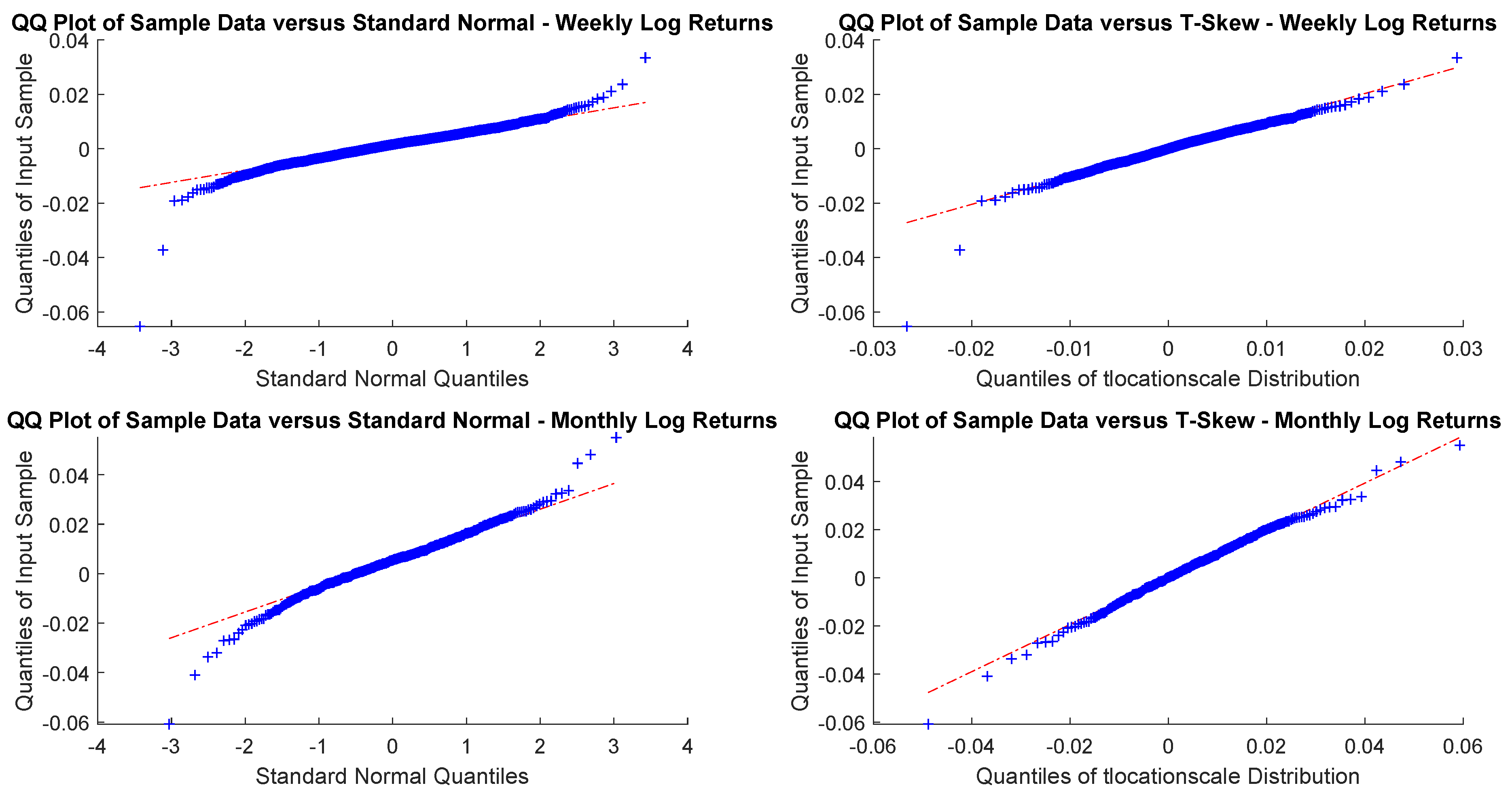(2020). This paper tries to help in gaining insights on returns’ distributions and on the most suitable way of fitting them. According to the empirical results we reported, the distributions that fit better the data are the t-skew and the hyperbolic Pareto. As the latter is more difficult to handle, this research suggests that the t-skew represents a suitable alternative. That is relevant in terms of policy implications because risk management or option pricing Mininni et al. (2020) should rely on models able to describe fat tails, skewed distributions and jumps in assets’ dynamics Orlando et al. (2018) rather than on Gaussian distributions that may underestimate the extremes (and leave the investors exposed to unexpected losses). For those reasons, regulators and financial institutions should pay particular attention to model risk (i.e., risk resulting from using insufficiently accurate models) when they choose a particular distribution.

Last but not least, t-skew models could be used as linkages between financial markets. To this end, Yoshiba (2018) provides a solution for computing the MLE and keeping the correlation matrix positive semi-definite during the optimization process.

Appendix A.1. Analysis on S&P 500 Index

Figure A1. S&P 500 log-returns histograms.

Figure A2. S&P 500 monthly and yearly log-returns Q-Q plots.

Figure A3. S&P 500 yearly windowed and yearly windowed shuffled log-returns Q-Q plots.

Figure A4. Empirical CDF versus standard normal CDF for S&P 500 returns. The dotted black lines represent the DKW upper and lower bounds.

Figure A5. S&P 500 log-returns autocorrelations.

Table A1. K-S test to detect the original distribution. The response is a boolean where 0 indicates that there is no evidence to reject the null hypothesis, and the value 1 is the opposite case.

	Normal			t-skew		Gen. Hyperbolic		Gen. Pareto		Exp. Pareto
	resp.	p-Value	DKW Exceeds	resp.	p-Value	resp.	p-Value	resp.	p-Value	resp.	p-Value
Weekly	1	1.6502 × 10${}^{-19}$	74.92%	0	0.0482	0	0.7256	1	0	1	0
Monthly	1	8.3615 × 10${}^{-9}$	58.32%	0	0.1985	0	0.9714	1	0	1	0
Yearly	1	2.7038 × 10${}^{-30}$	68.55%	1	8.6098 × 10${}^{-7}$	1	0	1	0	1	0
Yearly Shuffled	1	2.7038 × 10${}^{-30}$	68.55%	1	8.6098 × 10${}^{-7}$	1	0	1	0	1	0

Table A1. K-S test to detect the original distribution. The response is a boolean where 0 indicates that there is no evidence to reject the null hypothesis, and the value 1 is the opposite case.

	Normal			t-skew		Gen. Hyperbolic		Gen. Pareto		Exp. Pareto
	resp.	p-Value	DKW Exceeds	resp.	p-Value	resp.	p-Value	resp.	p-Value	resp.	p-Value
Weekly	1	1.6502 × 10${}^{-19}$	74.92%	0	0.0482	0	0.7256	1	0	1	0
Monthly	1	8.3615 × 10${}^{-9}$	58.32%	0	0.1985	0	0.9714	1	0	1	0
Yearly	1	2.7038 × 10${}^{-30}$	68.55%	1	8.6098 × 10${}^{-7}$	1	0	1	0	1	0
Yearly Shuffled	1	2.7038 × 10${}^{-30}$	68.55%	1	8.6098 × 10${}^{-7}$	1	0	1	0	1	0

Table A2. Ljung-Box Q-test and ARCH test to detect autocorrelation. The response is a boolean where 0 indicates that there is no evidence to reject the null hypothesis, and the value 1 is the opposite case.

	Ljung-Box Q-Test				ARCH Test
	$\mathit{m}=ln\left(\mathit{n}\right)$		$\mathit{m}=(\mathit{n}-\mathbf{1})$
	resp.	p-Value	resp.	p-Value	resp.	p-Value
Weekly	1	1.9720 × 10${}^{-5}$	1	0	1	0
Monthly	1	0.0031	1	0	1	0
Yearly	0	0.7234	1	0	0	0.2308
Yearly Shuffled	1	0	0	0.9306	1	0

Table A2. Ljung-Box Q-test and ARCH test to detect autocorrelation. The response is a boolean where 0 indicates that there is no evidence to reject the null hypothesis, and the value 1 is the opposite case.

	Ljung-Box Q-Test				ARCH Test
	$\mathit{m}=ln\left(\mathit{n}\right)$		$\mathit{m}=(\mathit{n}-\mathbf{1})$
	resp.	p-Value	resp.	p-Value	resp.	p-Value
Weekly	1	1.9720 × 10${}^{-5}$	1	0	1	0
Monthly	1	0.0031	1	0	1	0
Yearly	0	0.7234	1	0	0	0.2308
Yearly Shuffled	1	0	0	0.9306	1	0

Appendix A.2. Analysis on Bovespa Index

Figure A6. Bovespa log-returns histograms.

Figure A7. Bovespa monthly and yearly log-returns Q-Q plots.

Figure A8. Bovespa yearly windowed and yearly windowed shuffled log-returns Q-Q plots.

Figure A9. Empirical CDF versus standard normal CDF for Bovespa returns. The dotted black lines represent the DKW upper and lower bounds.

Figure A10. Bovespa log-returns autocorrelations.

Table A3. K-S test to detect the original distribution. The response is a boolean where 0 indicates that there is no evidence to reject the null hypothesis, and the value 1 is the opposite case.

	Normal			t-skew		Gen. Hyperbolic		Gen. Pareto		Exp. Pareto
	resp.	p-Value	DKW Exceeds	resp.	p-Value	resp.	p-Value	resp.	p-Value	resp.	p-Value
Weekly	1	4.0876 × 10${}^{-19}$	69.62%	0	0.7870	0	0.9870	1	0	1	0
Monthly	1	8.4152 × 10${}^{-7}$	31.55%	0	0.6679	0	0.9977	1	0	1	0
Yearly	1	6.7479 × 10${}^{-103}$	81.43%	1	3.7439 × 10${}^{-12}$	1	0	1	0	1	0
Yearly Shuffled	1	6.7479 × 10${}^{-103}$	81.43%	1	3.7439 × 10${}^{-12}$	1	0	1	0	1	0

Table A3. K-S test to detect the original distribution. The response is a boolean where 0 indicates that there is no evidence to reject the null hypothesis, and the value 1 is the opposite case.

	Normal			t-skew		Gen. Hyperbolic		Gen. Pareto		Exp. Pareto
	resp.	p-Value	DKW Exceeds	resp.	p-Value	resp.	p-Value	resp.	p-Value	resp.	p-Value
Weekly	1	4.0876 × 10${}^{-19}$	69.62%	0	0.7870	0	0.9870	1	0	1	0
Monthly	1	8.4152 × 10${}^{-7}$	31.55%	0	0.6679	0	0.9977	1	0	1	0
Yearly	1	6.7479 × 10${}^{-103}$	81.43%	1	3.7439 × 10${}^{-12}$	1	0	1	0	1	0
Yearly Shuffled	1	6.7479 × 10${}^{-103}$	81.43%	1	3.7439 × 10${}^{-12}$	1	0	1	0	1	0

Table A4. Ljung-Box Q-test and ARCH test to detect autocorrelation. The response is a boolean where 0 indicates that there is no evidence to reject the null hypothesis, and the value 1 is the opposite case.

	Ljung-Box Q-Test				ARCH Test
	$\mathit{m}=ln\left(\mathit{n}\right)$		$\mathit{m}=(\mathit{n}-\mathbf{1})$
	resp.	p-Value	resp.	p-Value	resp.	p-Value
Weekly	1	0	1	0	1	0
Monthly	1	0	1	0	1	1.3679 × 10${}^{-4}$
Yearly	1	0	1	0	1	0
Yearly Shuffled	0	0.8933	0	0.5147	0	0.7809

Table A4. Ljung-Box Q-test and ARCH test to detect autocorrelation. The response is a boolean where 0 indicates that there is no evidence to reject the null hypothesis, and the value 1 is the opposite case.

	Ljung-Box Q-Test				ARCH Test
	$\mathit{m}=ln\left(\mathit{n}\right)$		$\mathit{m}=(\mathit{n}-\mathbf{1})$
	resp.	p-Value	resp.	p-Value	resp.	p-Value
Weekly	1	0	1	0	1	0
Monthly	1	0	1	0	1	1.3679 × 10${}^{-4}$
Yearly	1	0	1	0	1	0
Yearly Shuffled	0	0.8933	0	0.5147	0	0.7809

Appendix A.3. Analysis on US Corporate Index

Figure A11. US Corp. log-returns histograms.

Figure A12. US Corp. monthly and yearly log-returns Q-Q plots.

Figure A13. US Corp. yearly windowed and yearly windowed shuffled log-returns Q-Q plots.

Figure A14. Empirical CDF versus standard normal CDF for US Corp. returns. The dotted black lines represent the DKW upper and lower bounds.

Figure A15. US Corp. log-returns autocorrelations.

Table A5. K-S test to detect the original distribution. The response is a boolean where 0 indicates that there is no evidence to reject the null hypothesis, and the value 1 is the opposite case.

	Normal			t-skew		Gen. Hyperbolic		Gen. Pareto		Exp. Pareto
	resp.	p-Value	DKW Exceeds	resp.	p-Value	resp.	p-Value	resp.	p-Value	resp.	p-Value
Weekly	1	0.0063	0.73%	0	0.3201	0	0.9748	1	0	1	0
Monthly	0	0.1877	0%	0	0.9965	0	0.9900	1	0	1	0
Yearly	0	0.0712	0%	0	0.0698	1	0	1	0	1	0
Yearly Shuffled	0	0.0712	0%	0	0.0698	1	0	1	0	1	0

Table A5. K-S test to detect the original distribution. The response is a boolean where 0 indicates that there is no evidence to reject the null hypothesis, and the value 1 is the opposite case.

	Normal			t-skew		Gen. Hyperbolic		Gen. Pareto		Exp. Pareto
	resp.	p-Value	DKW Exceeds	resp.	p-Value	resp.	p-Value	resp.	p-Value	resp.	p-Value
Weekly	1	0.0063	0.73%	0	0.3201	0	0.9748	1	0	1	0
Monthly	0	0.1877	0%	0	0.9965	0	0.9900	1	0	1	0
Yearly	0	0.0712	0%	0	0.0698	1	0	1	0	1	0
Yearly Shuffled	0	0.0712	0%	0	0.0698	1	0	1	0	1	0

Table A6. Ljung-Box Q-test and ARCH test to detect autocorrelation. The response is a boolean where 0 indicates that there is no evidence to reject the null hypothesis, and the value 1 is the opposite case.

	Ljung-Box Q-Test				ARCH Test
	$\mathit{m}=ln\left(\mathit{n}\right)$		$\mathit{m}=(\mathit{n}-\mathbf{1})$
	resp.	p-Value	resp.	p-Value	resp.	p-Value
Weekly	1	2.4980 × 10${}^{-14}$	1	0	1	6.0678 × 10${}^{-4}$
Monthly	0	0.7075	0	0.2615	1	4.8873 × 10${}^{-5}$
Yearly	1	0	1	0	1	0
Yearly Shuffled	0	0.2325	0	0.5581	0	0.7833

Table A6. Ljung-Box Q-test and ARCH test to detect autocorrelation. The response is a boolean where 0 indicates that there is no evidence to reject the null hypothesis, and the value 1 is the opposite case.

	Ljung-Box Q-Test				ARCH Test
	$\mathit{m}=ln\left(\mathit{n}\right)$		$\mathit{m}=(\mathit{n}-\mathbf{1})$
	resp.	p-Value	resp.	p-Value	resp.	p-Value
Weekly	1	2.4980 × 10${}^{-14}$	1	0	1	6.0678 × 10${}^{-4}$
Monthly	0	0.7075	0	0.2615	1	4.8873 × 10${}^{-5}$
Yearly	1	0	1	0	1	0
Yearly Shuffled	0	0.2325	0	0.5581	0	0.7833

Appendix A.4. Analysis on Emerging Markets Corporate Plus Index

Figure A16. EmMkt Corp. log-returns histograms.

Figure A17. EmMkt Corp. monthly and yearly log-returns Q-Q plots.

Figure A18. EmMkt Corp. yearly windowed and yearly windowed shuffled log-returns Q-Q plots.

Figure A19. Empirical CDF versus standard normal CDF for EmMkt Corp. returns. The dotted black lines represent the DKW upper and lower bounds.

Figure A20. EmMkt Corp. log-returns autocorrelations.

Table A7. K-S test to detect the original distribution. The response is a boolean where 0 indicates that there is no evidence to reject the null hypothesis, and the value 1 is the opposite case.

	Normal			t-skew		Gen. Hyperbolic		Gen. Pareto		Exp. Pareto
	resp.	p-Value	DKW Exceeds	resp.	p-value	resp.	p-Value	resp.	p-Value	resp.	p-Value
Weekly	1	8.3270 × 10${}^{-8}$	55.68%	0	0.8814	0	0.997	1	0	1	0
Monthly	1	0.0012	11.68%	0	0.9927	0	0.9999	1	0	1	0
Yearly	1	5.8695 × 10${}^{-4}$	8.54%	0	0.2340	1	0	1	0	1	0
Yearly Shuffled	0	0.0138	0%	0	0.3056	1	0	1	0	1	0

Table A7. K-S test to detect the original distribution. The response is a boolean where 0 indicates that there is no evidence to reject the null hypothesis, and the value 1 is the opposite case.

	Normal			t-skew		Gen. Hyperbolic		Gen. Pareto		Exp. Pareto
	resp.	p-Value	DKW Exceeds	resp.	p-value	resp.	p-Value	resp.	p-Value	resp.	p-Value
Weekly	1	8.3270 × 10${}^{-8}$	55.68%	0	0.8814	0	0.997	1	0	1	0
Monthly	1	0.0012	11.68%	0	0.9927	0	0.9999	1	0	1	0
Yearly	1	5.8695 × 10${}^{-4}$	8.54%	0	0.2340	1	0	1	0	1	0
Yearly Shuffled	0	0.0138	0%	0	0.3056	1	0	1	0	1	0

Table A8. Ljung-Box Q-test and ARCH test to detect autocorrelation. The response is a boolean where 0 indicates that there is no evidence to reject the null hypothesis, and the value 1 is the opposite case.

	Ljung-Box Q-Test				ARCH Test
	$\mathit{m}=ln\left(\mathit{n}\right)$		$\mathit{m}=(\mathit{n}-\mathbf{1})$
	resp.	p-Value	resp.	p-Value	resp.	p-Value
Weekly	1	0	1	0	1	0
Monthly	0	0.7652	0	0.9976	1	0.0018
Yearly	1	0	1	0	1	0
Yearly Shuffled	0	0.6017	1	0	0	0.9606

Table A8. Ljung-Box Q-test and ARCH test to detect autocorrelation. The response is a boolean where 0 indicates that there is no evidence to reject the null hypothesis, and the value 1 is the opposite case.

	Ljung-Box Q-Test				ARCH Test
	$\mathit{m}=ln\left(\mathit{n}\right)$		$\mathit{m}=(\mathit{n}-\mathbf{1})$
	resp.	p-Value	resp.	p-Value	resp.	p-Value
Weekly	1	0	1	0	1	0
Monthly	0	0.7652	0	0.9976	1	0.0018
Yearly	1	0	1	0	1	0
Yearly Shuffled	0	0.6017	1	0	0	0.9606

Appendix A.5. Analysis on 3-Month Treasury Constant Maturity Rate

Figure A21. DGS3M log-returns histograms.

Figure A22. DGS3M monthly and yearly log-returns Q-Q plots.

Figure A23. DGS3M yearly windowed and yearly windowed shuffled log-returns Q-Q plots.

Figure A24. Empirical CDF versus standard normal CDF for DGS3M returns. The dotted black lines represent the DKW upper and lower bounds.

Figure A25. DGS3M log-returns autocorrelations.

Table A9. K-S test to detect the original distribution. The response is a boolean where 0 indicates that there is no evidence to reject the null hypothesis, and the value 1 is the opposite case.

	Normal			t-skew		Gen. Hyperbolic		Gen. Pareto		Exp. Pareto
	resp.	p-Value	DKW Exceeds	resp.	p-Value	resp.	p-Value	resp.	p-Value	resp.	p-Value
Weekly	1	1.6567 × 10${}^{-20}$	47.48%	1	1.7558 × 10${}^{-20}$	1	1.46 × 10${}^{-20}$	1	0	1	0
Monthly	1	1.0664 × 10${}^{-71}$	75.69%	1	3.6783 × 10${}^{-7}$	1	0	1	0	1	0
Yearly	1	2.0644 × 10${}^{-286}$	79.83%	1	2.2533 × 10${}^{-26}$	1	0	1	0	1	0
Yearly Shuffled	1	3.0634 × 10${}^{-297}$	80.24%	1	1.3943 × 10${}^{-28}$	1	0	1	0	1	0

Table A9. K-S test to detect the original distribution. The response is a boolean where 0 indicates that there is no evidence to reject the null hypothesis, and the value 1 is the opposite case.

	Normal			t-skew		Gen. Hyperbolic		Gen. Pareto		Exp. Pareto
	resp.	p-Value	DKW Exceeds	resp.	p-Value	resp.	p-Value	resp.	p-Value	resp.	p-Value
Weekly	1	1.6567 × 10${}^{-20}$	47.48%	1	1.7558 × 10${}^{-20}$	1	1.46 × 10${}^{-20}$	1	0	1	0
Monthly	1	1.0664 × 10${}^{-71}$	75.69%	1	3.6783 × 10${}^{-7}$	1	0	1	0	1	0
Yearly	1	2.0644 × 10${}^{-286}$	79.83%	1	2.2533 × 10${}^{-26}$	1	0	1	0	1	0
Yearly Shuffled	1	3.0634 × 10${}^{-297}$	80.24%	1	1.3943 × 10${}^{-28}$	1	0	1	0	1	0

Table A10. Ljung-Box Q-test and ARCH test to detect autocorrelation. The response is a boolean where 0 indicates that there is no evidence to reject the null hypothesis, and the value 1 is the opposite case.

	Ljung-Box Q-Test				ARCH Test
	$\mathit{m}=ln\left(\mathit{n}\right)$		$\mathit{m}=(\mathit{n}-\mathbf{1})$
	resp.	p-Value	resp.	p-Value	resp.	p-Value
Weekly	1	0	1	0	1	0
Monthly	1	2.4962 × 10${}^{-4}$	1	0	1	0.0283
Yearly	1	0	1	0	1	0
Yearly Shuffled	1	3.0097 × 10${}^{-5}$	0	0.6966	1	0

Table A10. Ljung-Box Q-test and ARCH test to detect autocorrelation. The response is a boolean where 0 indicates that there is no evidence to reject the null hypothesis, and the value 1 is the opposite case.

	Ljung-Box Q-Test				ARCH Test
	$\mathit{m}=ln\left(\mathit{n}\right)$		$\mathit{m}=(\mathit{n}-\mathbf{1})$
	resp.	p-Value	resp.	p-Value	resp.	p-Value
Weekly	1	0	1	0	1	0
Monthly	1	2.4962 × 10${}^{-4}$	1	0	1	0.0283
Yearly	1	0	1	0	1	0
Yearly Shuffled	1	3.0097 × 10${}^{-5}$	0	0.6966	1	0

Appendix A.6. Analysis on 10-Year Treasury Constant Maturity Rate

Figure A26. DGS10Y log-returns histograms.

Figure A27. DGS10Y monthly and yearly log-returns Q-Q plots.

Figure A28. DGS10Y yearly windowed and yearly windowed shuffled log-returns Q-Q plots.

Figure A29. Empirical CDF versus standard normal CDF for DGS10Y returns. The dotted black lines represent the DKW upper and lower bounds.

Figure A30. DGS10Y log-returns autocorrelations.

Table A11. K-S test to detect the original distribution. The response is a boolean where 0 indicates that there is no evidence to reject the null hypothesis, and the value 1 is the opposite case.

	Normal			t-skew		Gen. Hyperbolic		Gen. Pareto		Exp. Pareto
	resp.	p-Value	DKW Exceeds	resp.	p-Value	resp.	p-Value	resp.	p-Value	resp.	p-Value
Weekly	1	1.2613 × 10${}^{-19}$	74.57%	0	0.7075	0	0.9404	1	0	1	0
Monthly	1	2.3517 × 10${}^{-6}$	39.47%	0	0.93367	0	0.9775	1	0	1	0
Yearly	1	3.2079 × 10${}^{-7}$	41.77%	1	0.0020	1	0	1	0	1	0
Yearly Shuffled	1	3.2079 × 10${}^{-7}$	41.77%	1	0.0020	1	0	1	0	1	0

Table A11. K-S test to detect the original distribution. The response is a boolean where 0 indicates that there is no evidence to reject the null hypothesis, and the value 1 is the opposite case.

	Normal			t-skew		Gen. Hyperbolic		Gen. Pareto		Exp. Pareto
	resp.	p-Value	DKW Exceeds	resp.	p-Value	resp.	p-Value	resp.	p-Value	resp.	p-Value
Weekly	1	1.2613 × 10${}^{-19}$	74.57%	0	0.7075	0	0.9404	1	0	1	0
Monthly	1	2.3517 × 10${}^{-6}$	39.47%	0	0.93367	0	0.9775	1	0	1	0
Yearly	1	3.2079 × 10${}^{-7}$	41.77%	1	0.0020	1	0	1	0	1	0
Yearly Shuffled	1	3.2079 × 10${}^{-7}$	41.77%	1	0.0020	1	0	1	0	1	0

Table A12. Ljung-Box Q-test and ARCH test to detect autocorrelation. The response is a boolean where 0 indicates that there is no evidence to reject the null hypothesis, and the value 1 is the opposite case.

	Ljung-Box Q-Test				ARCH Test
	$\mathit{m}=ln\left(\mathit{n}\right)$		$\mathit{m}=(\mathit{n}-\mathbf{1})$
	resp.	p-Value	resp.	p-Value	resp.	p-Value
Weekly	1	0	0	0.9879	1	0
Monthly	1	0.0248	0	0.9987	0	0.0721
Yearly	1	0	1	0	1	0
Yearly Shuffled	0	0.2294	1	0	0	0.5526

Table A12. Ljung-Box Q-test and ARCH test to detect autocorrelation. The response is a boolean where 0 indicates that there is no evidence to reject the null hypothesis, and the value 1 is the opposite case.

	Ljung-Box Q-Test				ARCH Test
	$\mathit{m}=ln\left(\mathit{n}\right)$		$\mathit{m}=(\mathit{n}-\mathbf{1})$
	resp.	p-Value	resp.	p-Value	resp.	p-Value
Weekly	1	0	0	0.9879	1	0
Monthly	1	0.0248	0	0.9987	0	0.0721
Yearly	1	0	1	0	1	0
Yearly Shuffled	0	0.2294	1	0	0	0.5526