


Abstract
The new class of matrix-tilted Archimedean copulas is introduced. It combines properties of Archimedean and elliptical copulas by introducing a tilting matrix in the stochastic representation of Archimedean copulas, similar to the Cholesky factor for elliptical copulas. Basic properties of this copula construction are discussed and a further extension outlined.
1. Introduction
Elliptical distributions are among the most important multivariate distributions and are widely used, for example, in finance, insurance, and risk management to model multivariate risk factor changes. A d-dimensional random vector is said to be elliptically distributed with location vector , if it admits the stochastic representation
where the (random) radial part is independent of the random vector which follows a uniform distribution on the Euclidean unit sphere and is a matrix of rank k (see Cambanis et al. (1981)); in what follows, we assume with and . Elliptical copulas are the copulas arising from elliptical distributions via Sklar’s Theorem; we assume the reader is familiar with the notion of copulas and related concepts of measuring dependence between the components of a random vector (see Nelsen 2006 for an introduction). Despite their popularity (partly due to the comparably simple simulation approach based on the stochastic representation (1)), elliptical copulas suffer from well-known limitations such as radial symmetry, which, in particular, implies that the lower and upper tail dependence coefficients are equal. This is often an unrealistic assumption from a practical point of view.
Another popular class of copulas are Archimedean copulas, which are copulas admitting the representation
for some known as (Archimedean) generator. McNeil and Nešlehová (2009) showed that a stochastic representation similar to (1) can be derived for Archimedean copulas. Archimedean copulas arise as survival copulas of random vectors with stochastic representation
where the radial part R is as in (1), independent of , but is now uniformly distributed on the standard simplex , that is, . The Archimedean generator corresponds to the Williamson d-transform of the radial part distribution of F and is given by
In contrast to elliptical copulas, Archimedean copulas are not restricted to radial symmetry. They are often given explicitly and properties can typically be described in terms of the generator . However, one major drawback is that they are exchangeable, which implies, for example, that all pairs of random variables share the same dependence structure. This might be unrealistic from a practical point of view (see Embrechts and Hofert 2011 for a discussion).
Analogously to the stochastic representation given in (1), the main contribution of this paper is to introduce a matrix A in the stochastic representation (2) which allows one to create asymmetric copulas which are limited to neither exchangeability nor radial symmetry. The construction of this new class of copulas, referred to as matrix-tilted Archimedean copulas, is given in Section 2. Section 3 discusses properties of matrix-tilted Archimedean copulas. Further extensions are mentioned in Section 4, while Section 5 concludes. All proofs are provided in the Appendix A. Other novel copula constructions not further discussed here include, for example, those in (Genest et al. 2018; Krupskii and Joe 2013, 2015; Quessy and Durocher 2019; Quessy et al. 2016).
2. The Construction
We are interested in the survival copulas of multivariate random vectors of the form
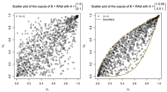
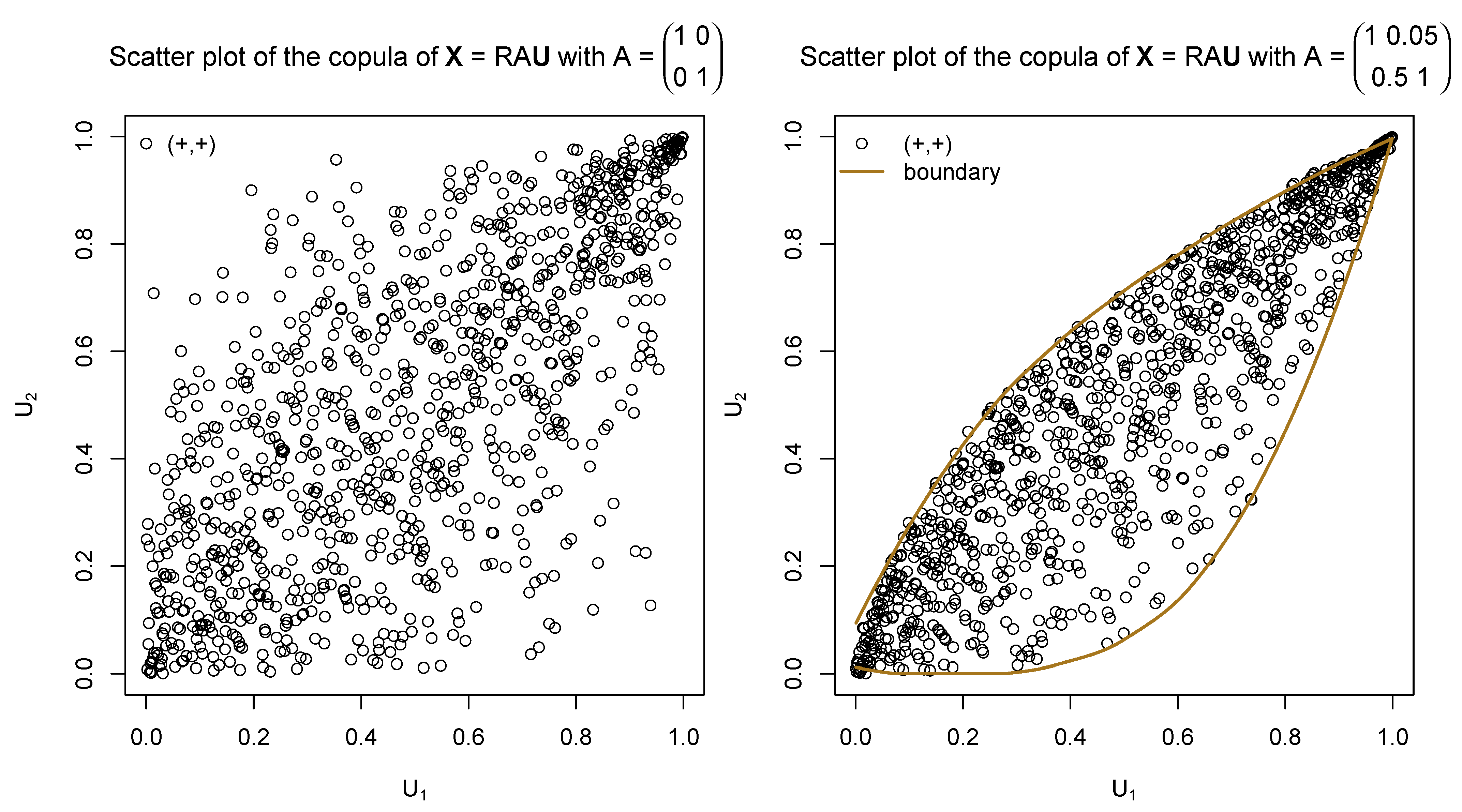
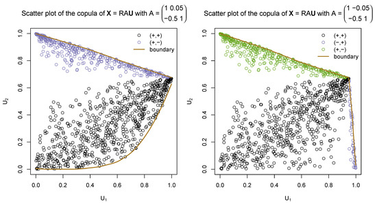
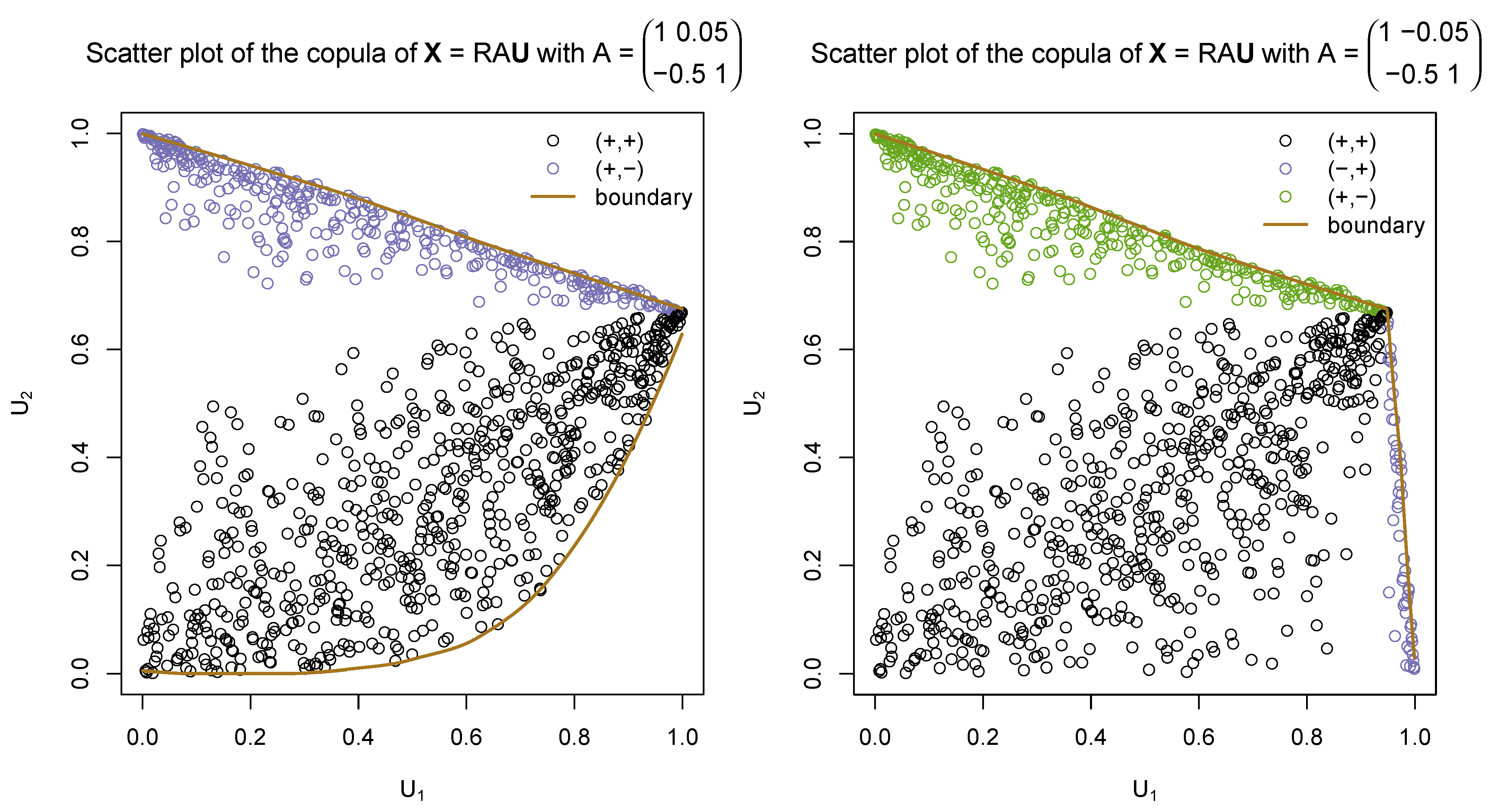
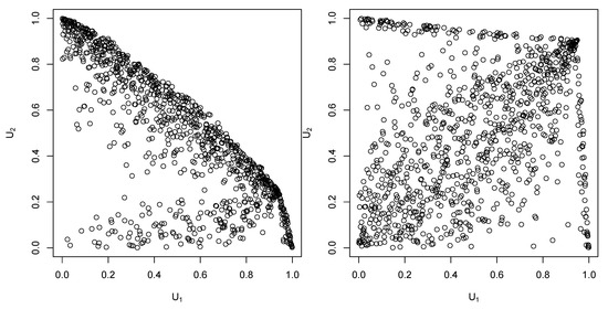
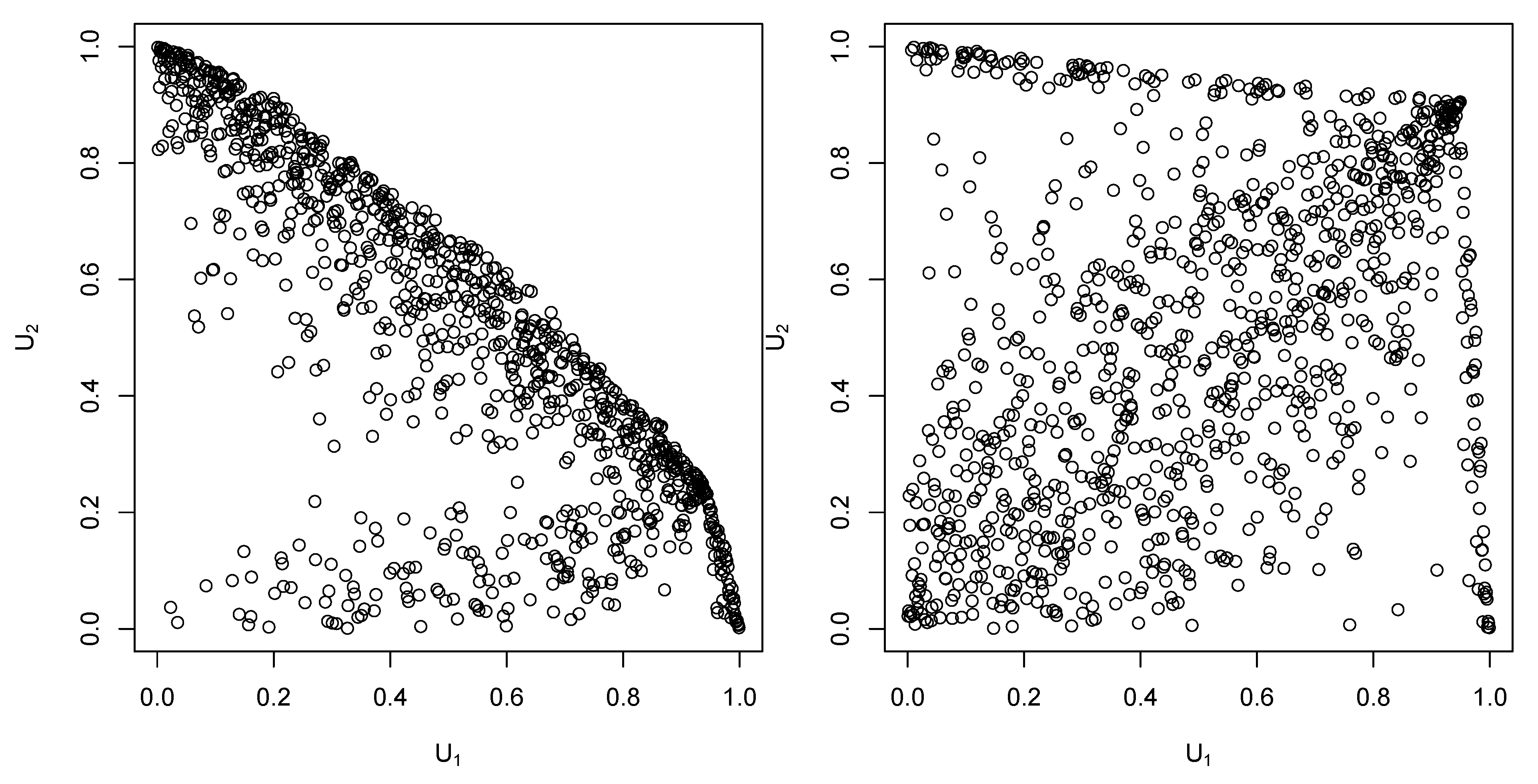
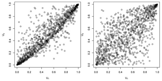
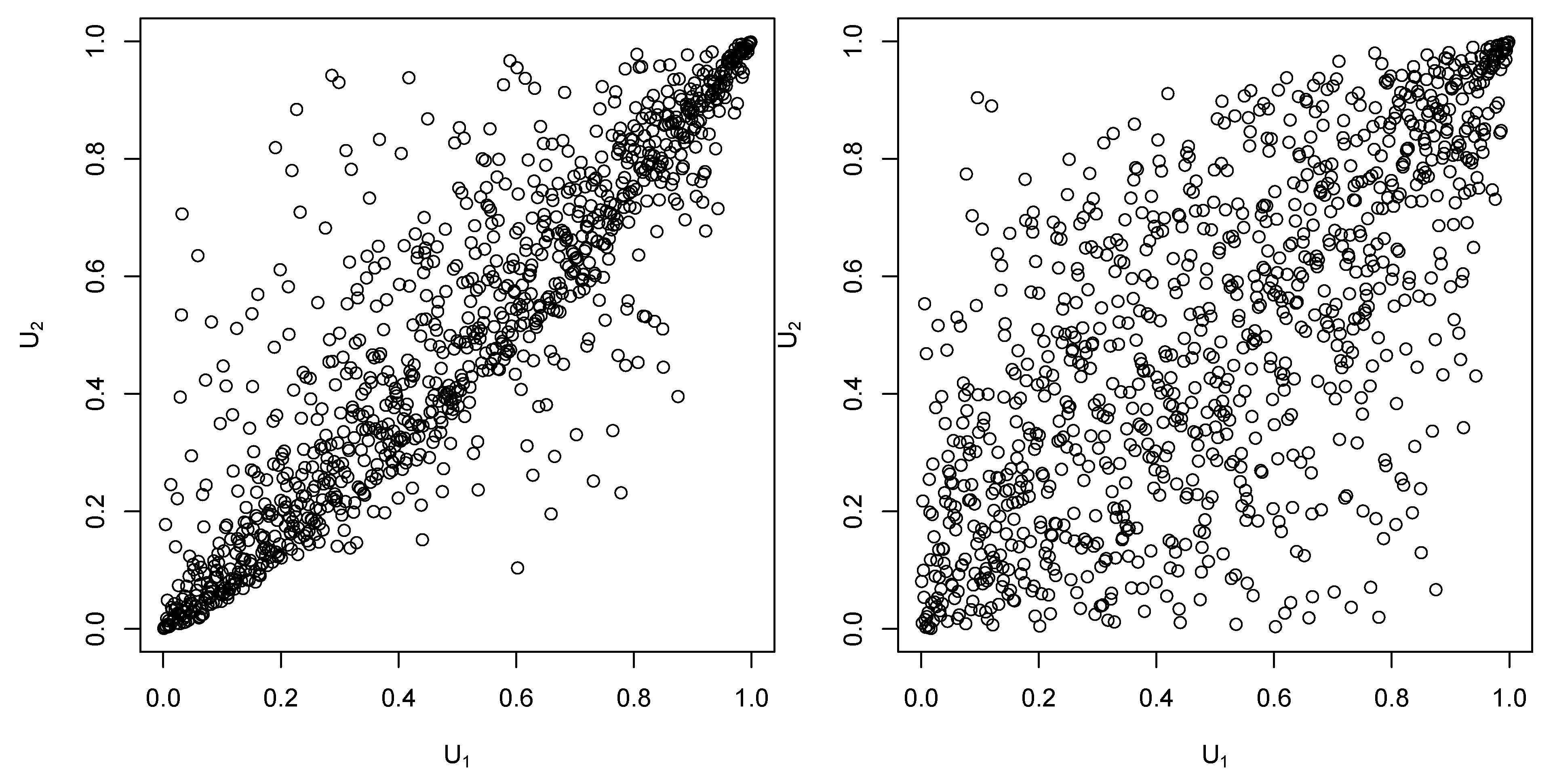
where R and are as above, and is a -matrix with real entries . The intuition behind the resulting dependence structure is the following. Naturally, our construction allows for asymmetric copulas; the degree of asymmetry could be quantified, for example, with the (scaled) supremal distance between the survival copula and copula of (4) (see Rosco and Joe 2013). For positive entries in A, mass gets squeezed towards the diagonal. For general entries, it is also possible to move mass towards the secondary diagonal. Depending on the different conditions imposed on A, the dependence structure of can vary substantially, which can make this construction interesting for scenario generation in risk applications. For example, Figure 1 and Figure 2 show samples of the empirical survival copula of in (4) based on the same 1000 realizations of R and but tilted with different matrices A; note that all scatter plots of samples of such type in this paper were generated in this way. The points are colored according to the quadrant the corresponding realization of lie in and the boundary curves of the support of the copula density is depicted.
Figure 1.
Scatter plots of 1000 samples from matrix-tilted Archimedean copulas with different tilting matrices A but otherwise equal realizations of R and . The plot on the left simply corresponds to a Gumbel copula with parameter (Kendall’s tau 0.5). The plot on the right also displays the boundary curves (spanned by ; see Proposition 1 below).
Figure 2.
Similar to Figure 1 with other tilting matrices A.
In what follows, we discuss a number of interesting cases and properties of matrix-tilted Archimedean copulas.
3. Properties
For the sake of tractability of the calculations and the fact that properties of multivariate copulas are often studied for bivariate margins (measures of association, tail dependence, symmetries, etc.), we focus on the bivariate case, that is, , and assume that
Section 3.1 addresses why Assumption (CPD) is natural. It often turns out to be useful to consider the random point
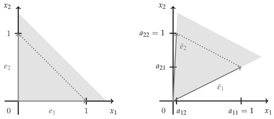
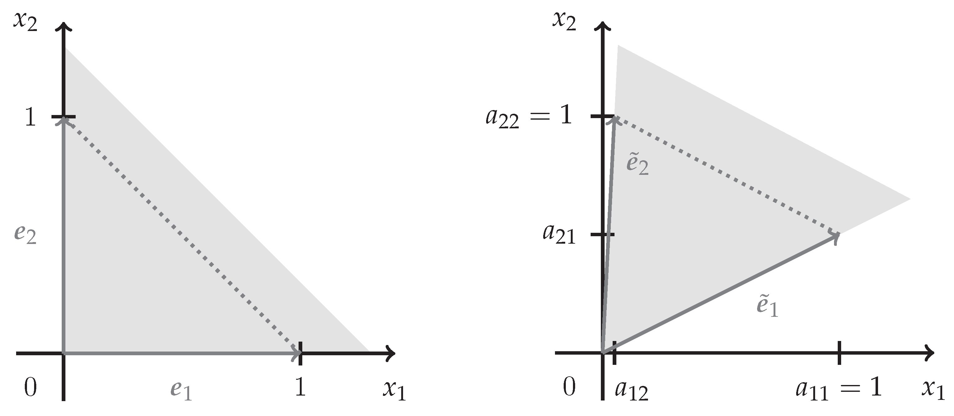
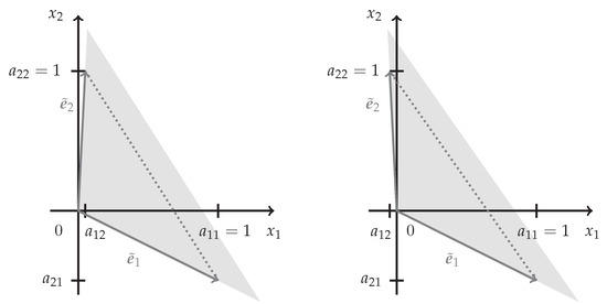
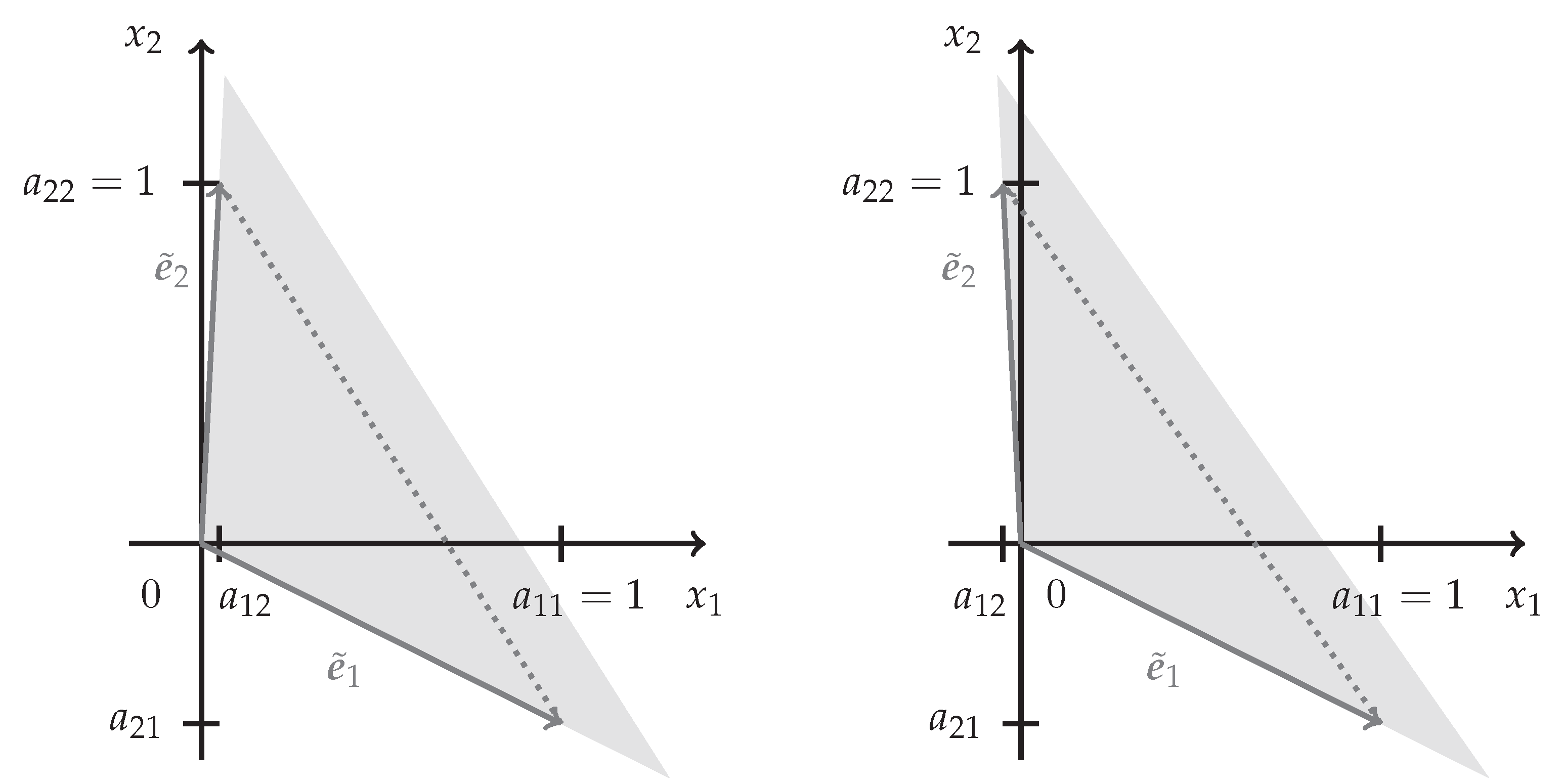
so the image of under A. All such images are denoted by their respective notation using a tilde. If , that is, the identity matrix in the bivariate case, then . The columns of A are in this case (the canonical basis vectors of ) and our construction simply leads to the class of Archimedean copulas. In the general case, A transforms to . Figure 3 and Figure 4 depict the space (randomly) spanned by (2) and (4), corresponding to Figure 1 and Figure 2.
Figure 3.
Depicting how (5) maps the vectors and to and , respectively, corresponding to Figure 1.
3.1. Special Cases
In this section, we briefly address various special cases of our construction and explain why Assumption (CPD) is natural.
First note that copulas are invariant under strictly increasing transformations of the margins. We can thus always multiply each component of by positive constants without losing flexibility of our dependence model; the same scaling is commonly used for elliptical copulas where one can assume A to be the Cholesky factor of a correlation (instead of a more general covariance) matrix. Therefore, we can equally well assume that , the first part of Assumption (CPD). The convex cone between the half-lines spanned by , , the columns of A, does not depend on the order of the columns in A. We can thus fix the determinant to be positive, the last part of Assumption (CPD). The assumptions and are for computational convenience. In the limiting case, when , we obtain and the corresponding matrix-tilted Archimedean copula is the upper Fréchet–Hoeffding bound M.
3.2. The Multivariate Survival Function
We can now provide the survival function of under Assumption (CPD).
Theorem 1.
- (i)
- If and , then
- (ii)
- If and , then
- (iii)
- If and , then
- (iv)
- If and , then
- (v)
- If and , then
The remaining cases can be obtained by exchanging the roles of and .
The following corollary considers two interesting special cases for the parameters and .
Corollary 1.
- (i)
- If and , then
- (ii)
- If , then, for , we haveand, for , we obtain that
3.3. The Boundary of the Support of the Copula Density
The following proposition provides almost sure boundaries for , the second component of in (4). The statements are directly clear from Figure 3 and Figure 4. The boundaries carry over to the boundaries for in the unit square after the map with the correct marginal survival functions (see also Figure 1 and Figure 2).
Proposition 1.
Under Assumption (CPD), the following inequalities hold almost surely for the component of of Model (4).
- (1)
- If , for all and for all .
- (2)
- If , for all .
- (3)
- If , for all .
3.4. Tail Dependence
In this section, we address the notion of tail dependence for the multivariate model as given in (4). Tail dependence is a copula property, so the coefficients of tail dependence only depend on the copula of (4). For the following result, note that a function is called regularly varying at of index (denoted by ) if
Proposition 2.
Let Assumption (CPD) hold and suppose that . Furthermore, let the marginal distribution of and be denoted by .
- (1)
- Let . If , then . If and at ∞, thenIf at 0, then
- (2)
- Let . If , then . If and at ∞, thenFurthermore, .
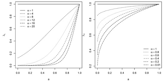
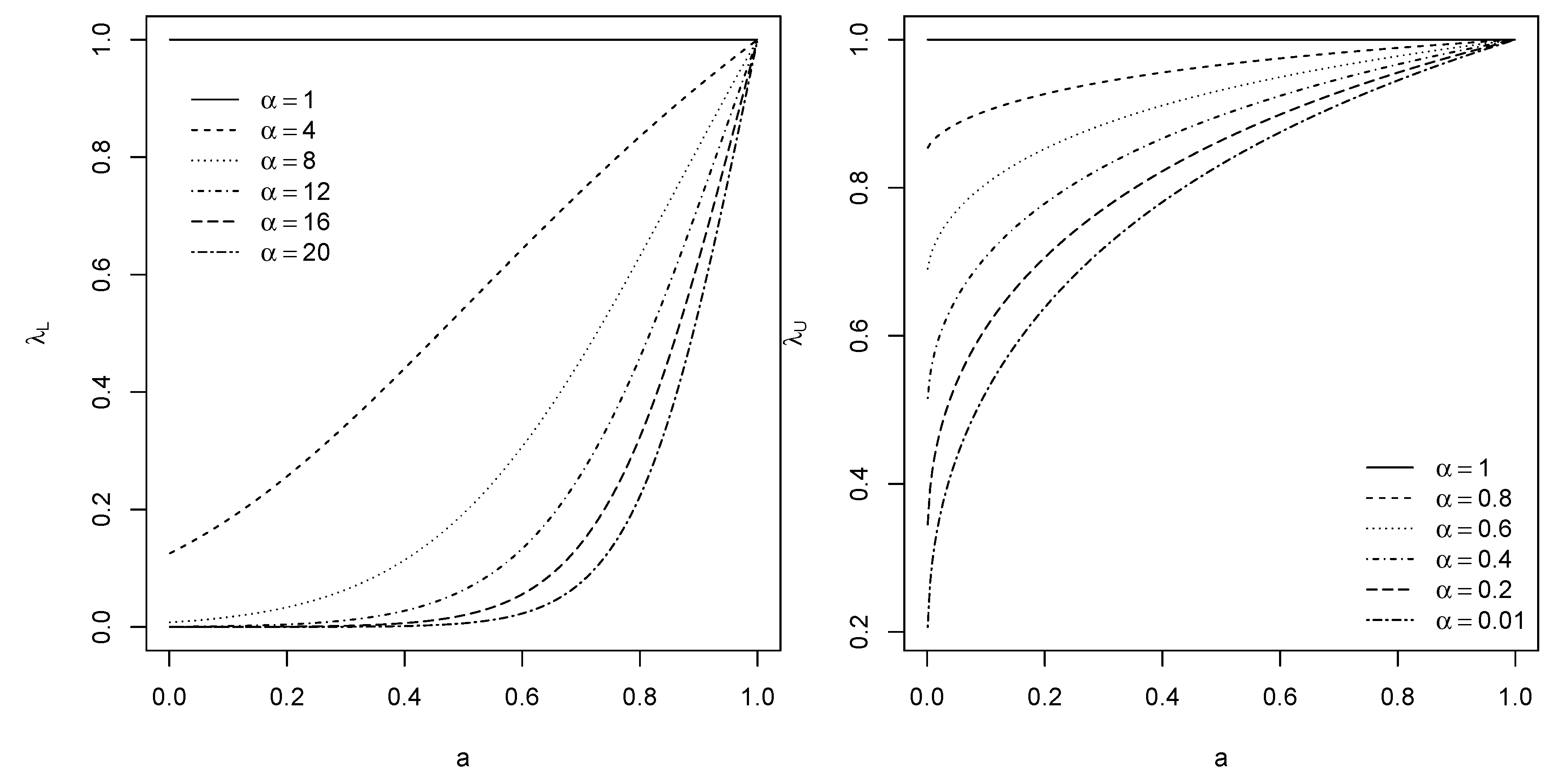
Figure 5.
and of Part (1) of Proposition 2 as functions of the parameter a for various α.
Assessing and in the case is more difficult. At least, the symmetric case can provide bounds. For example, if for all u sufficiently small, then (compare with the proof of Proposition 2)
and one can proceed as in the proof of Proposition 2 to evaluate (6); if for all u sufficiently small, then the inequality leads to a lower bound for .
4. Randomization and Other Extensions
As shown above, tilting an Archimedean copula through a matrix A makes the model more flexible by introducing different kinds of asymmetry. It is also possible to modify tail dependence properties through A. However, some parameter choices reduce the support of the copula to strict subsets of the unit square. This might be a desired feature for certain applications (a classical example is the copula of with almost surely), but equally well unnatural in others. A possible remedy may be to randomize the tilting matrix A; theoretical properties can then be derived by conditioning on A. While such random-matrix-tilted Archimedean copulas allow for very flexible models, inference is an open question.
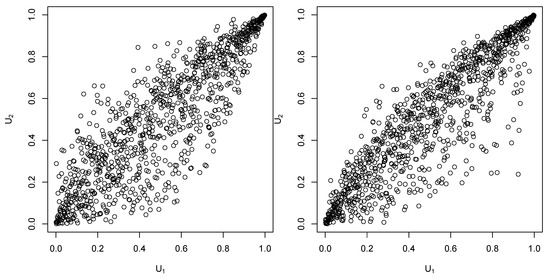
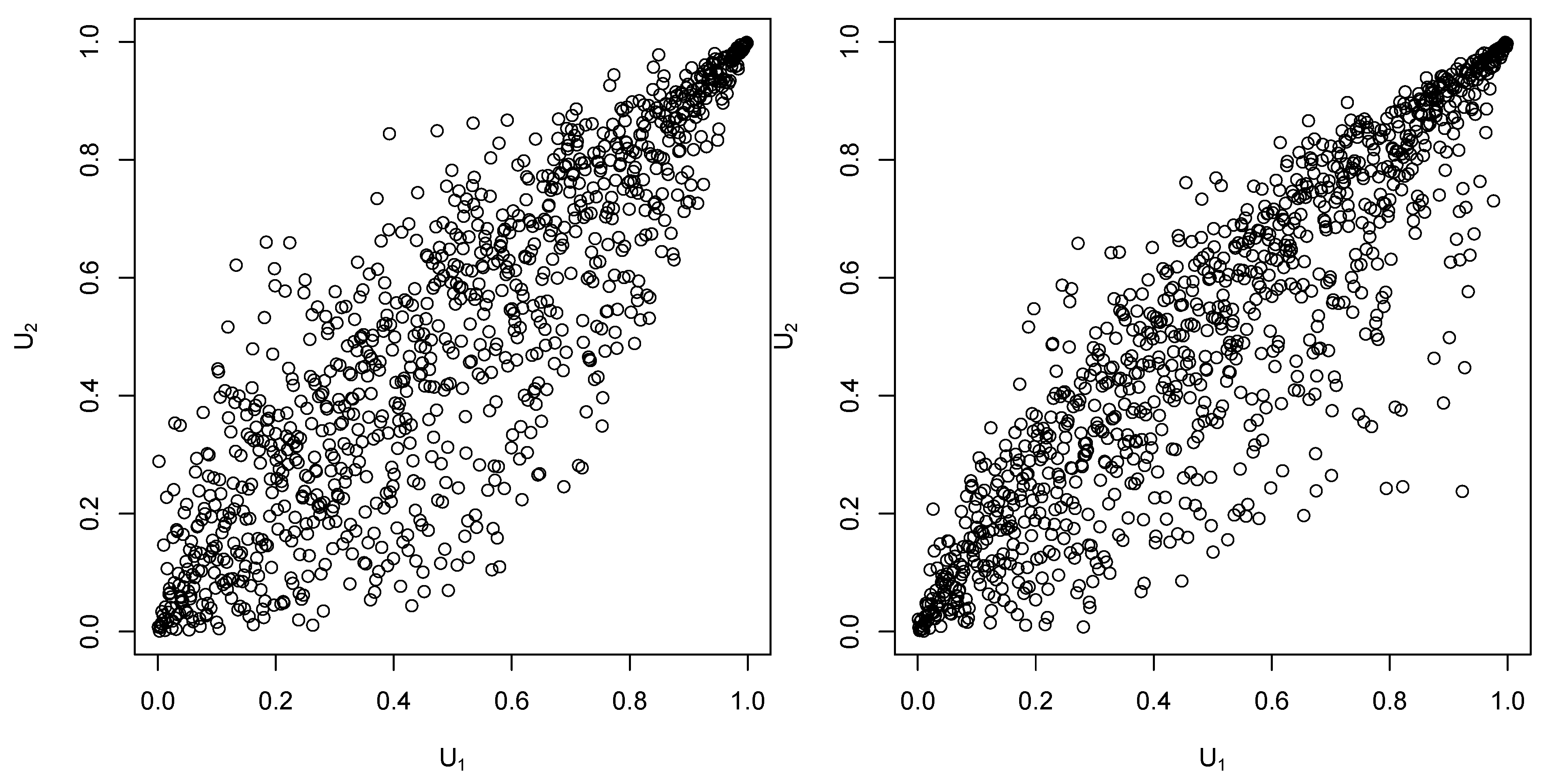
As a first example, we revisit the right-hand side of Figure 1 and randomize the entry of A with a standard uniform distribution. The result is shown on the left-hand side of Figure 6. Note that, although hardly visible here, the lower boundary as depicted on the right-hand side of Figure 1 still exists but the upper one is “washed out”. If we randomize both and , then both boundaries disappear. The right-hand side of Figure 6 shows such a case, where and are (independently) randomized by and distributions, respectively. Note that both of these randomizations satisfy Assumption (CPD).
Figure 6.
Scatter plots of 1000 samples from random-matrix-tilted Archimedean copulas with randomized entry (left) and independent , (right) based on the example displayed on the right-hand side of Figure 1.
As another example, let us consider the right-hand side of Figure 2 and randomize the entry of A via a uniform distribution on (see the left-hand side of Figure 7) or via with E being standard exponential (see the right-hand side of Figure 7). As above, both randomizations satisfy Assumption (CPD).
Another option not discussed here would be to make the randomized dependent by another copula.
A different approach to tilting (2) by a matrix A that we do not explore is the following. Consider a random vector
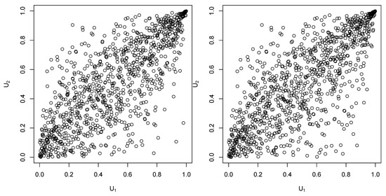
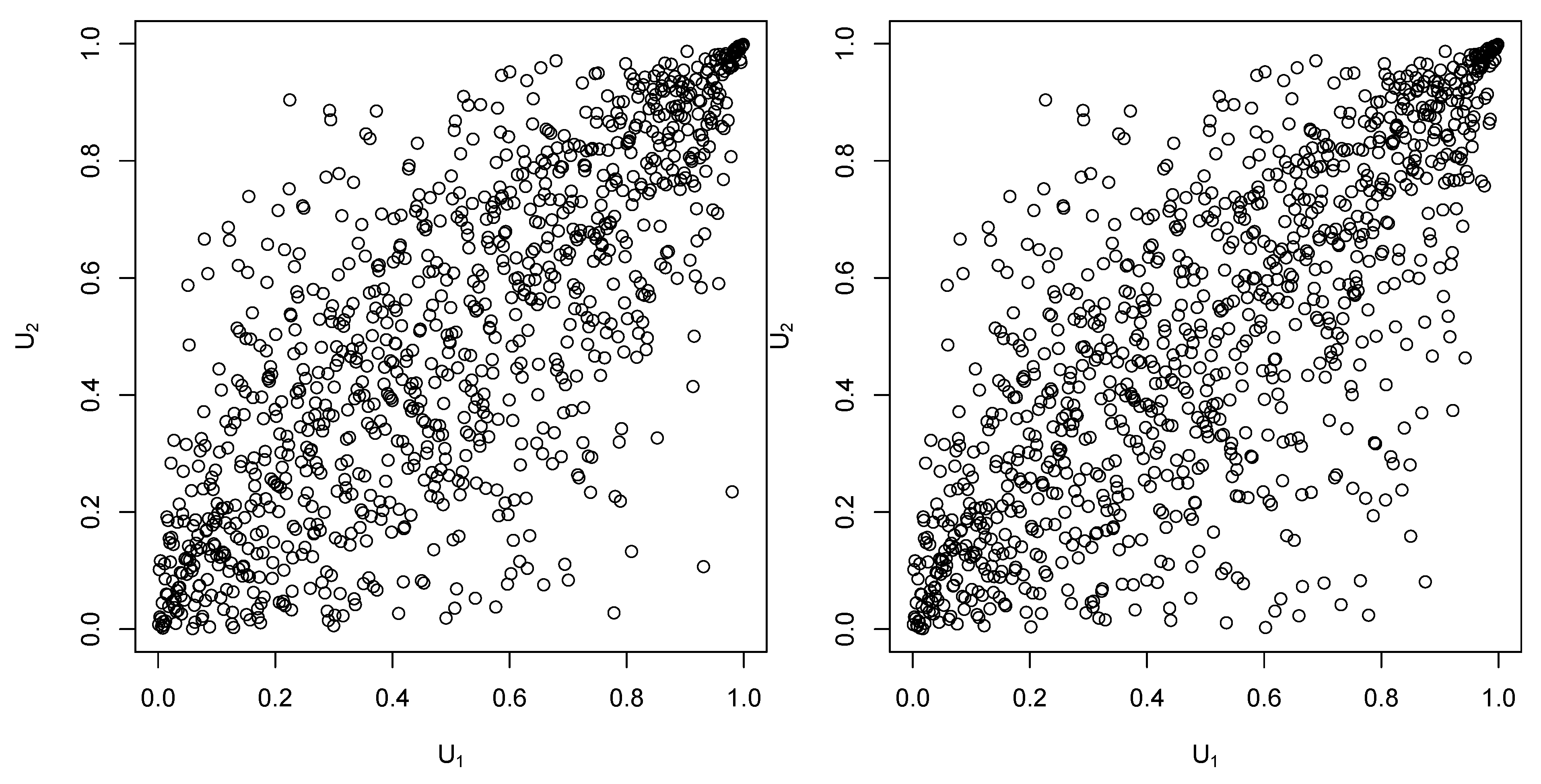
where R is a radial part as in (1), is uniformly distributed on the -sphere independently of R, and A is a -matrix. Then, one could consider the copula of the componentwise modulus of . Figure 8 and Figure 9 show the copulas of for R and A as chosen in Figure 2 and Figure 7, respectively, and given by (7). One observes that, for a deterministic tilting matrix A (see Figure 8), the construction does not seem to yield anything visually much different from a Gumbel copula (in distribution). We do not have proof of this fact but we have seen this behavior in all simulation examples.
Figure 8.
Scatter plots of the copulas of corresponding to Figure 2.
Figure 9.
Scatter plots of the copulas of corresponding to Figure 7.
The situation is more promising in the case of a randomized tiling matrix A (see Figure 9, especially the left-hand side).
5. Conclusions
Inspired by the construction of elliptical copulas, we present a new class of matrix-tilted Archimedean copulas, which generalize Archimedean copulas. Matrix-tilted Archimedean copulas are easy to simulate from and allow asymmetries to be modeled. In the bivariate case, the joint survival function and boundaries of the support of the multivariate model which gives rise to matrix-tilted Archimedean copulas can be given, and, in the case of equal margins and symmetric tilting matrix A, the tail dependence coefficients can be derived. Randomized tilting matrices A and the componentwise modulus of the model provide interesting extensions. Although their theoretical treatment is not straightforward, matrix-tilted Archimedean copulas are especially easy to incorporate into simulation-based applications.
The statistical estimation of matrix-tilted Archimedean copulas is an open problem for future research. A natural idea seems to be an iterative estimation procedure that alternates between finding an optimal Archimedean generator for the data given a specific tilting matrix and finding a best-fitting tilting matrix given the Archimedean generator of the previous step. In addition, random-matrix-tilted Archimedean copulas that do not limit the support to a strict subset of the unit hypercube may be of interest, too, as they may allow for likelihood optimization. Another avenue for future research is to introduce matrix tilting to generalizations of Archimedean copulas. One immediate generalization is to replace in (4) by a Dirichlet distribution which would then lead to matrix-tilted Liouville copulas.
Author Contributions
Conceptualization, M.H. and J.F.Z.; methodology, M.H. and J.F.Z.; formal analysis, M.H. and J.F.Z.; investigation, M.H. and J.F.Z.; writing—original draft preparation, M.H. and J.F.Z.; writing—review and editing, M.H. and J.F.Z.; visualization, M.H. and J.F.Z. All authors have read and agreed to the published version of the manuscript.
Funding
The first author’s research was funded by NSERC under Discovery Grant RGPIN-5010-2015.
Institutional Review Board Statement
Not applicable.
Informed Consent Statement
Not applicable.
Data Availability Statement
Not applicable.
Conflicts of Interest
The authors declare no conflict of interest.
Appendix A
The following proposition provides the survival function of , a result which is used in the proof of Theorem 1 below.
Proposition A1.
Let be uniformly distributed on . Under Assumption (CPD), we obtain that
Proof.
First, note that, for some ,
If and , then
Similarly, if and , we can interchange the role of and and obtain
which is as stated in the claim. From now on, assume and , and let . Then,
In the remaining part of the proof, we rewrite this expression to obtain the form as stated. Using and , multiplying out the terms, and noting that for all except the last term D (which easily follows from the bounds in the other indicators), we obtain that
where
Let
Basic calculations show that
so that with
In addition, implies that , with
As for B, we can decompose into with
Furthermore, can be written as , where
We thus obtain that
It is easy to see that . Finally, we can multiply with indicators that and obtain that
By first taking out and consecutively pulling together the terms, we obtain that
which, by a basic calculation, leads to the claim as stated. □
The following lemma is an auxiliary result, which is also used in the proof of Theorem 1.
Lemma A1.
Let and . Then,
with the convention that for (and similarly for the term involving b).
Proof.
First, assume . Writing , we obtain that
so it suffices to consider the first integral. For , this gives . If , we have
Hence,
Applying the same idea with a replaced by and putting the pieces together, we obtain that
Now, assume . Then,
so that we can apply the formula for the case with here. This implies that
which is of the form as stated in this case. Finally, if , then the integral is 0. Again, it is easy to see that the result as stated is indeed 0 in this case. □
We can now address the proof of Theorem 1.
Proof of Theorem 1.
We consider several cases.
Case 1: and .
By Proposition A1,
The fraction in the integrand can be written as and thus the whole integral as , with
By distinguishing the cases , , and , we obtain that
Note that, if , then . This implies that
By splitting up F in a similar fashion, we obtain that
Distinguishing the cases of different sign of in the last integral leads to
Note that the first and third integrald on the right-hand side of the last equation can be pulled together. In addition, note that the second integral can be written as
Applying Lemma A1 leads to
Recalling that the result is , we obtain the form as claimed.
Case 2: and .
This case directly follows from Case 1 by interchanging and , as well as and .
Case 3: and .
Since , let us first consider the integrand. By Proposition A1, we have that
where
It is straightforward to check that
We now consider four different cases.
This can be rewritten as
Furthermore, implies that
so that
Similarly, we obtain that
Summarizing the terms leads to
Since and , we have
Consider the case . If , then , so that . If and , then our above assumptions imply that , a contradiction. Thus, if . Similarly, if . This implies that
For , we have if . Thus, for , we have that
Similarly,
Integrating the terms now leads to
Case 3.2: and .
It is straightforward to check that, in this case,
so that
For B, note that and imply that . For , . Furthermore, , and imply that . Therefore,
Thus,
Similarly,
Note that, in our case here, because
but the right-hand side is less than or equal to . In addition, if , we have that , because, otherwise (), we have , which then leads to , a contradiction (note that ). This implies that
Case 3.3: and .
Let . If , then , so . If , then , thus and therefore . This implies that and thus that , so this indicator drops out of the term A. In addition, note that implies for . Hence, the corresponding indicator in the term A is also always one. We therefore obtain that
By considering the cases of different signs for , we can write the term B as
If and , then , so . By summarizing the indicators, this yields
Since if and , it follows that
Similarly, for C,
Note that the indicator function drops out, since, if and , then . The second summand of indicators completely vanishes, since, if and , then implies . If , the contradiction follows. We thus obtain that
Pulling the terms together, we obtain that
Distinguishing the cases and , we obtain that
Note that and . We show next that . To this end, let . If , then implies that and thus . If , then a contradiction follows immediately. Otherwise, we see that . This yields in contradiction to the assumption that . If , then yields a contradiction immediately. Therefore, and hence . Similarly, if and , we show that . To this end, let . Then, , so that , and thus . The case directly leads to a contradiction. If , then , which implies that . As above, this leads to a contradiction to the assumption that . Thus, . Plugging in these relations and summarizing the terms, we obtain that
Integrating the terms now leads to
Case 3.4: and .
Interchanging the roles of , and , , we obtain that
□
Finally, here is the proof of Proposition 2.
Proof of Proposition 2.
(1) Recall that for as in (4). Then,
Under the given assumptions, note that the distribution of is supported in the first quadrant, the marginal survival functions are equal (denoted by ), and, for , we have by Corollary 1 that
Therefore, we obtain that
Let .
Since and ψ is non-increasing, for all . Furthermore, there exists an such that the numerator of (A4) is zero but the denominator is greater than zero for all . Hence .
If , applying l’Hôpital’s Rule leads to
Dividing by and using regular variation, we obtain that
Now, consider and note that
Using (A2) and (A3), and proceeding similarly as above (with regular variation at 0), one obtains as stated.
(2) Under the given assumptions, using Corollary 1, we obtain that
This yields
If , then . If , then l’Hôpital’s Rule and regular variation imply that
Now, consider and note that the margins live on . Similar to above, we obtain that
which is easily seen to be 0.
□
References
- Cambanis, Stamatis, Steel Huang, and Gordon Simons. 1981. On the theory of elliptically contoured distributions. Journal of Multivariate Analysis 11: 368–85. [Google Scholar] [CrossRef] [Scilit]
- Embrechts, Paul, and Marius Hofert. 2011. Comments on: Inference in multivariate Archimedean copula models. TEST 20: 263–70. [Google Scholar] [CrossRef] [Scilit]
- Genest, Christian, Johanna Nešlehová, and Louis-Paul Rivest. 2018. The class of multivariate max-id copulas with ℓ1-norm symmetric exponent measure. Bernoulli 24: 3751–90. [Google Scholar] [CrossRef] [Scilit]
- Krupskii, Pavel, and Harry Joe. 2013. Factor copula models for multivariate data. Journal of Multivariate Analysis 120: 85–101. [Google Scholar] [CrossRef] [Scilit]
- Krupskii, Pavel, and Harry Joe. 2015. Structured factor copula models: Theory, inference and computation. Journal of Multivariate Analysis 138: 53–73. [Google Scholar] [CrossRef] [Scilit]
- McNeil, Alexander J., and Johanna Nešlehová. 2009. Multivariate Archimedean copulas, d-monotone functions and l1-norm symmetric distributions. The Annals of Statistics 37: 3059–97. [Google Scholar] [CrossRef] [Scilit]
- Nelsen, Roger B. 2006. An Introduction to Copulas. Berlin/Heidelberg: Springer. [Google Scholar]
- Quessy, Jean-François, and Martin Durocher. 2019. The class of copulas arising from squared distributions: Properties and inference. Econometrics and Statistics 12: 148–66. [Google Scholar] [CrossRef] [Scilit]
- Quessy, Jean-François, Louis-Paul Rivest, and Marie-Hélène Toupin. 2016. On the family of multivariate chi-square copulas. Journal of Multivariate Analysis 152: 40–60. [Google Scholar] [CrossRef] [Scilit]
- Rosco, J. F., and Harry Joe. 2013. Measures of tail asymmetry for bivariate copulas. Statistical Papers 54: 709–26. [Google Scholar] [CrossRef] [Scilit]
Publisher’s Note: MDPI stays neutral with regard to jurisdictional claims in published maps and institutional affiliations. |
© 2021 by the authors. Licensee MDPI, Basel, Switzerland. This article is an open access article distributed under the terms and conditions of the Creative Commons Attribution (CC BY) license (https://creativecommons.org/licenses/by/4.0/).