Dynamic Optimal Mean-Variance Portfolio Selection with a 3/2 Stochastic Volatility

Abstract

This paper considers a mean-variance portfolio selection problem when the stock price has a 3/2 stochastic volatility in a complete market. Specifically, we assume that the stock price and the volatility are perfectly negative correlated. By applying a backward stochastic differential equation (BSDE) approach, closed-form expressions for the statically optimal (time-inconsistent) strategy and the value function are derived. Due to time-inconsistency of mean variance criterion, a dynamic formulation of the problem is presented. We obtain the dynamically optimal (time-consistent) strategy explicitly, which is shown to keep the wealth process strictly below the target (expected terminal wealth) before the terminal time. Finally, we provide numerical studies to show the impact of main model parameters on the efficient frontier and illustrate the differences between the two optimal wealth processes.

1. Introduction

In the last several decades, various stochastic volatility models have been developed in the literature to explain the volatility smile and heavy tails of return distribution as widely observed in the financial market; see, for example, Heston (1993); Hull and White (1987); Lewis (2000); and Stein and Stein (1991). Among them, a non-affine model with a mean reverting structure called the 3/2 stochastic volatility model Lewis (2000) enjoys empirical support in the bond and stock market by previous works, such as Ahn and Gao (1999); Bakshi et al. (2006); and Jones (2003). Effort has been made under the 3/2 stochastic volatility in derivative pricing problems such as Carr and Sun (2007); Drimus (2012); and Yuen et al. (2015). It seems, however, that little attention has been paid to portfolio selection problems under Markowitz (1952) mean-variance criterion.

The single-period asset allocation theory under the mean-variance criterion is first introduced by the seminal paper Markowitz (1952). Thereafter, there has been increasing attention on extensions and applications of Markowitz’s work. Two milestones are the work of Li and Ng (2000) and Zhou and Li (2000) that generalize Markowitz’s work to a multi-period and continuous-time setting by using embedding techniques. In Zhou and Li (2000), they assume that all the market parameters are deterministic functions or constants. To extend the results to more realistic models with random parameters, on the assumption that the return rate, volatility, and risk premium are all bounded stochastic processes, the backward stochastic differential equation (BSDE) approach is introduced by Lim and Zhou (2002) to solve a mean-variance problem in a complete market. From then on, many papers work on the mean-variance portfolio selection problem under various financial models by using the BSDE approach. Chiu and Wong (2011) consider the problem where asset prices are cointegrated. Shen et al. (2014) investigate the same problem under a constant elasticity of variance model by assuming that the risk premium process satisfies an exponential integrability. Zhang and Chen (2016) extend the results in Shen et al. (2014) by further incorporating a liability process. Shen and Zeng (2015) study the optimal investment-reinsurance problem for a mean-variance insurer in an incomplete market where the risk premium process is proportional to a Markovian, affine-form, and square-root process, and a modified locally square-integrable optimal strategy is derived by imposing an exponential integrability of order 2 on the risk premium process. Under similar conditions considered in Shen and Zeng (2015), a mean-variance problem under the Heston model with a liability process and a financial derivative is considered in Li et al. (2018). Other relevant works on mean-variance portfolio selection problems by applying not only the BSDE approach, but also other approaches (for example, the dynamic programming approach and the martingale approach Pliska (1986)) include Bielecki et al. (2005); Chang (2015); Ferland and Watier (2010); Han and Wong (2020); Lv et al. (2016); Pan and Xiao (2017); Pan et al. (2018); Peng and Chen (2020a, 2020b); Shen (2015, 2020); Shen et al. (2020); Tian et al. (2021); and Yu (2013).

The literature mentioned above under Markowitz’s paradigm, however, shares one characteristic, that is, all deals with pre-committed strategies Strotz (1956). The resulting optimal strategy always depends on the initial wealth level, and thus is called time-inconsistent. Recently, the time-consistent mean-variance portfolio selection problem has received considerable attention. To tackle the time-inconsistency, Basak and Chabakauri (2010) derive a time-consistent strategy which is determined by applying a backward recursion starting from the terminal date. Björk et al. (2017) develop a game theoretical approach under Markovian settings which essentially studies the subgame-perfect Nash equilibrium, and they derive the equilibrium strategy and equilibrium value function by solving an extended Hamilton–Jacobi–Bellman (HJB) equation. Along this approach, previous works include Li et al. (2012, 2015); Lin and Qian (2016); and Zhu and Li (2020), to name but only a few. Alternatively, Pedersen and Peskir (2017) introduce the dynamically optimal approach to investigate the time-inconsistency of mean-variance problems. They overcome the time-inconsistency by recomputing the statically optimal (pre-committed) strategy during the investment period, and they can therefore obtain dynamically optimal (time-consistent) strategies by solving infinitely many optimization problems.

Motivated by these aspects, we consider a dynamic mean-variance portfolio selection problem within the framework developed in Pedersen and Peskir (2017) in a complete market with two primitive assets: a risk-free asset and a stock with 3/2 stochastic volatility. In particular, the market is completed by fixing a perfectly negative correlation between the stock price and the volatility. To make the problem analytically tractable, the return rate of the stock is a constant so that the risk premium process is linear in the reciprocal of volatility process. We adopt the BSDE approach to solve this problem. The Lagrange multiplier is first applied to transform the mean-variance problem into an unconstrained optimization problem. By making an assumption on model parameters, the uniqueness and existence of solution to a special type BSDE Bender and Kohlmann (2000) is established. We then solve the BSDE explicitly and obtain the optimal strategy in a closed-form for the unconstrained optimization problem. Furthermore, we derive the analytic expression of the statically optimal strategy of the mean-variance portfolio selection problem by the Lagrange duality theorem. Finally, by solving the statically optimal strategy at each time, we obtain the dynamically optimal strategy which is shown to keep the corresponding wealth process strictly below the target (expected terminal wealth) before the terminal time. To summarize, this paper has main contributions in three aspects: (1) We make an assumption on the model parameters instead of on the risk premium process. This assumption guarantees the existence and uniqueness of solutions to the BSDEs. (2) We manage to derive the square-integrable optimal strategy instead of the locally square-integrable optimal strategy and verify the admissibility. (3) We provide both the static and dynamic optimality.

The rest of this paper is organized as follows. Section 2 formulates the financial market and the portfolio selection problem. In Section 3, we derive the explicit solutions to the BSDEs as well as the closed-from expression of the optimal investment strategy of the unconstrained problem. Section 4 presents the static and dynamic optimality of the mean-variance portfolio selection problem. In Section 5, we provide numerical examples to present the efficient frontier under the statically optimal strategy and illustrate the differences between the two optimal controlled wealth processes. Section 6 concludes the paper.

2. Formulation of the Problem

Let $[0,T]$ be a finite horizon and $(\Omega ,\mathcal{F},\mathrm{P})$ be a complete probability space which carries a one-dimensional standard Brownian motion $W={\left(W_t\right)}_{t\in [0,T]}$. The right-continuous, $\mathrm{P}$-complete filtration ${\left({\mathcal{F}}_t\right)}_{t\in [0,T]}$ is generated by the Brownian motion W.

We consider a market where two primitive assets—one risk-free asset and one stock—are available to the investor. The price of the risk-free asset B solves

$$d{B}_t=r{B}_{t}dt,$$

with $B_{t_0}=b_0\in {\mathbb{R}}^{+}$ at time $t_0\in [0,T)$ fixed and given, where $r>0$ stands for the interest rate. The price of the stock follows

$$d{S}_t=\mu S_{t}dt+\sqrt{V_t}{S}_{t}d{W}_t,$$

(1)

with $S_{t_0}=s_0\in {\mathbb{R}}^{+}$ at time $t_0$. The return rate of the stock price $\mu >r$ is a constant and $V={\left(V_t\right)}_{t\in [t_0,T]}$ is the stochastic variance of the stock price described by a 3/2 model (see, for example, Lewis (2000)):

$$d{V}_t=\kappa V_t(\theta -V_t)dt-\sigma V_t^{3/2}d{W}_t,$$

(2)

with the initial value of $V_{t_0}=v_0\in {\mathbb{R}}^{+}$ at time $t_0$, where three parameters, $\kappa ,\theta$, and $\sigma$, are all assumed to be positive. We hereby put the minus sign in front of $\sigma$ in (2) to emphasize the assumption that the dynamics of the stock price $S_t$ and the volatility $V_t$ are perfectly negative correlated.

We shall consider Markov controls $u(t,V_t,X_t^u)$ denoting the wealth invested in the stock at time $t\in [t_0,T]$, and such a deterministic function $u(·,·,·)$ is called a feedback control law. We assume that there are no transaction costs in the trading as well as other restrictions. The investor wishes to create a self-financing portfolio of the risk-free asset B and the stock S dynamically. Thus, the controlled wealth process ${\left(X_t^u\right)}_{t\in [t_0,T]}$ of the investor can be described by the system of SDEs below.

$$\begin{array}{c}\hfill \left\{\begin{array}{cc}\hfill d{X}_t^u& =[r{X}_t^u+(\mu -r)u(t,V_t,X_t^u)]dt+u(t,V_t,X_t^u)\sqrt{V_t}d{W}_t,\hfill \\ \hfill d{V}_t& =\kappa V_t(\theta -V_t)dt-\sigma V_t^{3/2}d{W}_t,\hfill \end{array}\right.\end{array}$$

(3)

with $X_{t_0}^u=x_0$ at time $t_0\in [0,T)$. We let ${\mathrm{P}}_{t_0,v_0,x_0}$ denote the probability measure with initial value $(V_{t_0},X_{t_0}^u)=(v_0,x_0)$ at time $t_0\in [0,T)$.

Definition 1.

Given any fixed $t_0\in [0,T)$, if for any $(v_0,x_0)\in {\mathbb{R}}^{+}\times \mathbb{R}$, it holds that

1. 

${\mathrm{E}}_{t_0,v_0,x_0}\left[{\int }_{t_0}^T{u}^2(t,V_t,X_t^u)V_{t}dt\right]<\infty$,

2. 

${\mathrm{E}}_{t_0,v_0,x_0}\left[{sup}_{t\in [t_0,T]}{\left|X_t^u\right|}^2\right]<\infty$,

then the (Markovian) strategy u is called admissible. We denote by $\mathcal{U}$ the set of admissible portfolio strategies.

We are first interested in determining an admissible strategy $u\in \mathcal{U}$ that solves the following portfolio problem:

Definition 2.

The mean-variance portfolio problem is an optimization problem denoted by

$$\begin{array}{c}\hfill \left\{\begin{array}{cc}\hfill \underset{u\in \mathcal{U}}{min}& {\mathrm{Var}}_{t_0,v_0,x_0}\left(X_T^u\right)\hfill \\ \hfill \mathrm{subject}\mathrm{to}& {\mathrm{E}}_{t_0,v_0,x_0}\left[X_T^u\right]=\xi ,\hfill \end{array}\right.\end{array}$$

(4)

where ξ is a fixed and given constant playing the financial role of a target. The corresponding value function is denoted by $V_{MV}(t_0,v_0,x_0)$.

Remark 1.

Here, we impose $\xi >x_0{e}^{r(T-t_0)}$, in line with previous studies such as Lim and Zhou (2002); Shen and Zeng (2015), and Shen et al. (2014). Otherwise, the investor can simply take the risk-free strategy $u\equiv 0$ over $[t_0,T]$ which dominates any other admissible strategy.

As a result of the quadratic nonlinearity of the variance operator, problem (4) falls outside of Bellman’s principle. Denote by $u^{\ast }$ the optimal strategy in problem (4) which refers to the static optimality (refer to Definition 1 in Pedersen and Peskir (2017)) and is relative to the initial position $(t_0,v_0,x_0)$. The investor might not be committed to the statically optimal strategy $u^{\ast }$ chosen at the very initial position $(t_0,v_0,x_0)$ during the following investment period $(t_0,T]$. Therefore, we shall also consider a dynamic formulation of problem (4). Here, we opt for the framework developed in Pedersen and Peskir (2017). We now review the definition of dynamic optimality in problem (4) for the readers’ convenience.

Definition 3.

For a triple $(t_0,v_0,x_0)\in [0,T)\times {\mathbb{R}}^{+}\times \mathbb{R}$ fixed and given, we call a Makrov strategy $u^{d\ast }$ dynamically optimal in problem (4), if for every $(t,v,x)\in [t_0,T)\times {\mathbb{R}}^{+}\times \mathbb{R}$ and every strategy $\pi \in \mathcal{U}$ with $\pi (t,v,x)\ne u^{d\ast }(t,v,x)$ and ${\mathrm{E}}_{t,v,x}\left[X_T^{\pi }\right]=\xi$, there is a Markov strategy w satisfying $w(t,v,x)=u^{d\ast }(t,v,x)$ and ${\mathrm{E}}_{t,v,x}\left[X_T^w\right]=\xi$ such that

$${\mathrm{Var}}_{t,v,x}\left(X_T^w\right)<{\mathrm{Var}}_{t,v,x}\left(X_T^{\pi }\right).$$

The dynamically optimal strategy $u^{d\ast }$ is essentially derived by solving the statically optimal strategy $u^{\ast }$ at each time and implementing it in an infinitesimally small period of time, which in turn implies that we shall first address problem (4) in the sense of static optimality so as to derive the dynamic optimality.

We observe that problem (4) is, in fact, a convex optimization problem with linear constraint ${\mathrm{E}}_{t_0,v_0,x_0}\left[X_T^u\right]=\xi$. Thus, we can handle the constraint by introducing a Lagrange multiplier $\theta \in \mathbb{R}$, and define the following Lagrangian:

$$\begin{array}{cc}\hfill L(x_0,v_0;u,\theta )& ={\mathrm{E}}_{t_0,v_0,x_0}\left[{(X_T^u-\xi )}^2\right]+2\theta {\mathrm{E}}_{t_0,v_0,x_0}[X_T^u-\xi ]\hfill \\ \hfill & ={\mathrm{E}}_{t_0,v_0,x_0}\left[{(X_T^u-(\xi -\theta ))}^2\right]-{\theta }^2.\hfill \end{array}$$

(5)

Then, the Lagrangian duality theorem (see, for example, Luenberger (1968)) indicates that we can derive the static optimality $u^{\ast }$ in problem (4) by solving the following equivalent min-max stochastic control problem:

$$\underset{\theta \in \mathbb{R}}{max}\underset{u\in \mathcal{U}}{min}L(x_0,v_0;u,\theta ).$$

(6)

This shows that we can solve problem (6) with two steps, of which the first step is to solve the unconstrained stochastic optimization problem with respect to $u\in \mathcal{U}$ given a fixed $\theta \in \mathbb{R}$ and the second step is to solve the static optimization problem with respect to the Lagrange multiplier $\theta \in \mathbb{R}$. Therefore, we can first address the following unconstrained quadratic-loss minimization problem:

$$\underset{u\in \mathcal{U}}{min}J(x_0,v_0;u,\gamma )={\mathrm{E}}_{t_0,v_0,x_0}\left[{(X_T^u-\gamma )}^2\right],$$

(7)

with $\gamma =\xi -\theta$ fixed and given.

3. Solution to the Unconstrained Problem

In this section, we opt for the BSDE approach so as to solve problem (7) above. Before formulating the main results in this section, we make the following notations to facilitate the discussions below. For any ${\mathbb{R}}^{+}$-valued, ${\mathcal{F}}_t$-adapted stochastic process $\eta :={\left({\eta }_t\right)}_{t\in [0,T]}$, a continuous process $A:={\left(A_t\right)}_{t\in [0,T]}$ associated with $\eta$ is defined by $A_t={\int }_0^t{\eta }_s^{2}ds$. Let $\beta \ge 0$ be a generic constant, we denote by

• $L_{\mathrm{P}}^2(\beta ,\eta ,[0,T];\mathbb{R})$: the space of ${\mathcal{F}}_t$-adapted, $\mathbb{R}$-valued stochastic processes f satisfying

  $${\parallel f\parallel }_{\beta }^2:=\mathrm{E}\left[{\int }_0^T{e}^{\beta A_t}{\left|f_t\right|}^{2}dt\right]<\infty ;$$
• $L_{\mathrm{P}}^{2,\eta }(\beta ,\eta ,[0,T];\mathbb{R})$: the space of ${\mathcal{F}}_t$-adapted, $\mathbb{R}$-valued stochastic processes f satisfying

  $${\parallel \eta f\parallel }_{\beta }^2:=\mathrm{E}\left[{\int }_0^T{\eta }_t^2{e}^{\beta A_t}{\left|f_t\right|}^{2}dt\right]<\infty ;$$
• $L_{\mathrm{P}}^{2,c}(\beta ,\eta ,[0,T];\mathbb{R})$ the space of ${\mathcal{F}}_t$-adapted, $\mathbb{R}$-valued stochastic processes f satisfying

  $${\parallel f\parallel }_{\beta ,c}^2:=\mathrm{E}\left[\underset{0\le t\le T}{sup}{e}^{\beta A_t}{\left|f_t\right|}^2\right]<\infty .$$

Therefore, we have the following Banach space:

$$\mathcal{M}(\beta ,\eta ,[0,T];{\mathbb{R}}^2):=(L_{\mathrm{P}}^{2,\eta }(\beta ,\eta ,[0,T];\mathbb{R}))\cap (L_{\mathrm{P}}^{2,c}(\beta ,\eta ,[0,T];\mathbb{R}))\times (L_{\mathrm{P}}^2(\beta ,\eta ,[0,T];\mathbb{R})$$

with the norm ${\parallel (Y,Z)\parallel }_{\beta }^2={\parallel \eta Y\parallel }_{\beta }^2+{\parallel Y\parallel }_{\beta ,c}^2+{\parallel Z\parallel }_{\beta }^2$.

In addition, we introduce

$$\begin{array}{c}\hfill \left\{\begin{array}{cc}\hfill \Delta =& {[\kappa \theta +2(\mu -r)\sigma ]}^2-2{\sigma }^2{(\mu -r)}^2,\hfill \\ \hfill n_1=& \frac{-[\kappa \theta +2(\mu -r)\sigma ]+\sqrt{\Delta }}{-{\sigma }^2},\hfill \\ \hfill n_2=& \frac{-[\kappa \theta +2(\mu -r)\sigma ]-\sqrt{\Delta }}{-{\sigma }^2},\hfill \\ \hfill C_b=& max\left\{(60+16\sqrt{14})\left({(\mu -r)}^2+\frac{{\sigma }^2{n}_1^2{n}_2^2{(1-e^{\sqrt{\Delta }T})}^2}{{(n_1-n_2{e}^{\sqrt{\Delta }T})}^2}\right),\right.\hfill \\ \hfill & \left.8{(\mu -r)}^2+8(\mu -r)\sigma \frac{n_1{n}_2(1-e^{\sqrt{\Delta }T})}{n_1-n_2{e}^{\sqrt{\Delta }T}}\right\}.\hfill \end{array}\right.\end{array}$$

(8)

It can be easily checked that $\Delta >0$ due to $\mu >r$. The following standing assumption is imposed on the model parameters throughout the paper:

Assumption 1.

$C_b\le {\kappa }^2{\theta }^2/2{\sigma }^2$.

Remark 2.

It follows from Lemma 5 below that $C_b$ is strictly increasing in T. In particular, when $T\to 0$, $C_b\to (60+16\sqrt{14}){(\mu -r)}^2$. This indicates the feasibility of Assumption 1. Moreover, Assumption 1 is crucial to guarantee that three BSDEs—(9), (12), and (17)—admit unique solutions and the statically optimal strategy (30) is admissible.

The following linear BSDE of $(P,\Gamma )$ is considered so as to solve problem (7):

$$\begin{array}{c}\hfill \left\{\begin{array}{cc}\hfill d{P}_t& =\left\{\left[2r-\frac{{(\mu -r)}^2}{V_t}\right]P_t+\frac{2(\mu -r)}{\sqrt{V_t}}{\Gamma }_t\right\}dt+{\Gamma }_{t}d{W}_t,\hfill \\ \hfill P_T& =1.\hfill \end{array}\right.\end{array}$$

(9)

Clearly, due to the randomness and unboundedness of the driver of (9), this linear BSDE is without the uniform Lipschitz continuity with respect to both $P_t$ and ${\Gamma }_t$. Thus, BSDE (9) is out of scope of EI Karoui et al. (1997). Nevertheless, we observe that BSDE (9) follows a stochastic Lipschitz continuity which is first proposed in Bender and Kohlmann (2000). To proceed, some useful results on the BSDE with the stochastic Lipschitz continuity adapted from Definition 2 and Theorem 3 in Bender and Kohlmann (2000) are presented below.

Definition 4.

We call a pair $(\zeta ,f)$ standard data for the BSDE of $(Y,Z)$:

$$\left\{\begin{array}{cc}\hfill -d{Y}_t& =f(t,Y_t,Z_t)dt-Z_{t}d{W}_t,\hfill \\ \hfill Y_T& =\zeta ,t\in [0,T],\hfill \end{array}\right.$$

if the following four conditions hold:

1. 

There exist two ${\mathbb{R}}^{+}$-valued, ${\mathcal{F}}_t$-adapted stochastic processes ${\left({\eta }_{1,t}\right)}_{t\in [0,T]}$ and ${\left({\eta }_{2,t}\right)}_{t\in [0,T]}$ such that $\forall t\in [0,T],\forall (y_1,z_1),(y_2,z_2)\in {\mathbb{R}}^2$

$$|f(t,y_1,z_1)-f(t,y_2,z_2)|\le {\eta }_{1,t}|y_1-y_2|+{\eta }_{2,t}|z_1-z_2|.$$

We refer to this inequality as the stochastic Lipschitz continuity.

2. 

There exists a positive constant $\epsilon >0$ satisfying ${\eta }_t^2:={\eta }_{1,t}+{\eta }_{2,t}\ge \epsilon$.

3. 

The terminal condition ζ satisfies $\mathrm{E}\left[\exp \left(\beta {\int }_0^T{\eta }_t^{2}dt\right){\left|\zeta \right|}^2\right]<\infty$ in which β is a positive constant.

4. 

$\frac{f(·,0,0)}{\eta }\in L_{\mathrm{P}}^2(\beta ,\eta ,[0,T];\mathbb{R})$.

Lemma 1.

The BSDE of $(Y,Z)$

$$\left\{\begin{array}{cc}\hfill -d{Y}_t& =f(t,Y_t,Z_t)dt-Z_{t}d{W}_t,\hfill \\ \hfill Y_T& =\zeta ,t\in [0,T],\hfill \end{array}\right.$$

admits a unique solution $(Y,Z)\in \mathcal{M}(\beta ,\eta ,[0,T];{\mathbb{R}}^2)$ if $(\zeta ,f)$ is standard data for a sufficiently large β, in particular, for $\beta >3+\sqrt{21}$.

Before adapting the above results to establish the uniqueness and existence of the solution to BSDE (9), we recall the following useful result from Theorem 5.1 in Zeng and Taksar (2013).

Lemma 2.

Suppose the process ${\left(r_t\right)}_{t\in [0,T]}$ follows the Cox–Ingersoll–Ross (CIR) model:

$$d{r}_t=(\kappa \theta -\kappa r_t)dt+\sigma \sqrt{r_t}d{W}_t,$$

where $\kappa ,\theta$ and σ are positive constants. Then, we have

$$\mathrm{E}\left[\exp \left(\beta {\int }_0^T{r}_{t}dt\right)\right]<\infty ifandonlyif\beta \le {\kappa }^2/2{\sigma }^2.$$

Lemma 3.

Assume Assumption 1 holds, then there is a constant $3+\sqrt{21}<\beta \le \frac{{\kappa }^2{\theta }^2}{6{(\mu -r)}^2{\sigma }^2}$ such that the unique solution $(P,\Gamma )\in \mathcal{M}(\beta ,\eta ,[t_0,T];{\mathbb{R}}^2)$ with ${\eta }_t={\left(2r+\frac{3{(\mu -r)}^2}{V_t}\right)}^{1/2}$ to BSDE (9) exists.

Proof. 

Let ${\eta }_{1,t}=2r-{(\mu -r)}^2/V_t$ and ${\eta }_{2,t}=2(\mu -r)/\sqrt{V_t}$. Denote in this case the non-negative ${\mathcal{F}}_t$-adapted process ${\eta }_t$ by

$${\eta }_t^2:={\eta }_{1,t}+{\eta }_{2,t}^2,$$

and accordingly, define the increasing process $A_t$ by

$$A_t:={\int }_{t_0}^t{\eta }_s^{2}ds={\int }_{t_0}^t\left(2r+\frac{3{(\mu -r)}^2}{V_s}\right)ds.$$

We then have

$$\begin{array}{cc}\hfill {\mathrm{E}}_{t_0,v_0,x_0}\left[\exp \left(\beta A_T\right)\right]& \le C{\mathrm{E}}_{t_0,v_0,x_0}\left[\exp \left(3{(\mu -r)}^2\beta {\int }_{t_0}^T\frac{1}{V_t}dt\right)\right],\hfill \end{array}$$

where the positive constant $C>0$ is independent of $\beta$. By Itô’s lemma, we then have the following dynamics of the reciprocal of the variance process (2):

$$d\left(\frac{1}{V_t}\right)=\kappa \theta \left(\frac{\kappa +{\sigma }^2}{\kappa \theta }-\frac{1}{V_t}\right)dt+\sigma \sqrt{\frac{1}{V_t}}d{W}_t,$$

which is a CIR process. It follows from Lemma 2 that if

$$3{(\mu -r)}^2\beta \le \frac{{\kappa }^2{\theta }^2}{2{\sigma }^2},$$

then we have

$${\mathrm{E}}_{t_0,v_0,x_0}\left[\exp \left(3{(\mu -r)}^2\beta {\int }_{t_0}^T\frac{1}{V_t}dt\right)\right]<\infty .$$

Indeed, when Assumption 1 holds, there exists a constant $\beta$ such that $3+\sqrt{21}<\beta \le \frac{{\kappa }^2{\theta }^2}{6{(\mu -r)}^2{\sigma }^2}$, and the driver and the terminal condition of BSDE (9) then constitute standard data. Finally, by Lemma 1 above, we see that a unique solution $(P,\Gamma )\in \mathcal{M}(\beta ,\eta ,[t_0,T];{\mathbb{R}}^2)$ to BSDE (9) with $3+\sqrt{21}<\beta \le \frac{{\kappa }^2{\theta }^2}{6{(\mu -r)}^2{\sigma }^2}$ and ${\eta }_t={\left(2r+\frac{3{(\mu -r)}^2}{V_t}\right)}^{1/2}$ exists. □

In what follows, we shall give the explicit expression of the unique solution $(P,\Gamma )$ of BSDE (9).

Lemma 4.

Assume Assumption 1 holds, then the unique solution $(P,\Gamma )$ of BSDE (9) has the following explicit expression:

$$\begin{array}{c}\hfill \left\{\begin{array}{cc}\hfill P_t& =\exp \left(-2r(T-t)\right)g(t,V_t),\hfill \\ \hfill {\Gamma }_t& =\sigma a\left(t\right)\frac{P_t}{\sqrt{V_t}},\hfill \end{array}\right.\end{array}$$

(10)

for $t\in [t_0,T]$, where $g(t,v)=\exp \left\{a\left(t\right)\frac{1}{v}+b\left(t\right)\right\}$, and $a\left(t\right)$ and $b\left(t\right)$ are solutions to the following system of ODEs:

$$\begin{array}{c}\hfill \left\{\begin{array}{cc}\frac{da\left(t\right)}{dt}-(\kappa \theta +2(\mu -r)\sigma )a\left(t\right)+\frac{1}{2}{\sigma }^2{a}^2\left(t\right)+{(\mu -r)}^2=0,\hfill & \hfill a\left(T\right)=0,\\ \frac{db\left(t\right)}{dt}+(\kappa +{\sigma }^2)a\left(t\right)=0,\hfill & \hfill b\left(T\right)=0.\end{array}\right.\end{array}$$

(11)

Proof. 

We first introduce the likelihood process ${\left(L_t\right)}_{t\in [t_0,T]}$ from the dynamics

$$d{L}_t=-\frac{2(\mu -r)}{\sqrt{V_t}}{L}_{t}d{W}_t,L_{t_0}=1.$$

Similar to the reasoning in Lemma 3, it can be easily verified from Assumption 1 above that

$${\mathrm{E}}_{t_0,v_0,x_0}\left[\exp \left({\int }_{t_0}^T\frac{2{(\mu -r)}^2}{V_t}dt\right)\right]<\infty .$$

That is, the Novikov’s condition is satisfied for ${\left(L_t\right)}_{t\in [t_0,T]}$. Thus, ${\left(L_t\right)}_{t\in [t_0,T]}$ is a uniformly integrable martingale under ${\mathrm{P}}_{t_0,v_0,x_0}$ measure and we can define an equivalent probability measure ${\tilde{\mathrm{P}}}_{t_0,v_0,x_0}$ on ${\mathcal{F}}_T$ through the Radon–Nikodym derivative

$$d{\tilde{\mathrm{P}}}_{t_0,v_0,x_0}=L_{T}d{\mathrm{P}}_{t_0,v_0,x_0}.$$

From the Girsanov’s theorem, Brownian motions under ${\tilde{\mathrm{P}}}_{t_0,v_0,x_0}$ and ${\mathrm{P}}_{t_0,v_0,x_0}$ are related to each other through

$$d{W}_t^{\tilde{\mathrm{P}}}=\frac{2(\mu -r)}{\sqrt{V_t}}dt+d{W}_t,$$

and we can rewrite (9) under the ${\tilde{\mathrm{P}}}_{t_0,v_0,x_0}$-measure as follows:

$$\begin{array}{c}\hfill \left\{\begin{array}{cc}\hfill d{P}_t& =\left\{\left[2r-\frac{{(\mu -r)}^2}{V_t}\right]P_t\right\}dt+{\Gamma }_{t}d{W}_t^{\tilde{\mathrm{P}}},\hfill \\ \hfill P_T& =1.\hfill \end{array}\right.\end{array}$$

(12)

We see that the driver of BSDE (12) again satisfies the stochastic Lipschitz continuity with, in this case, ${\eta }_t^2=|2r-\frac{{(\mu -r)}^2}{V_t}|+\epsilon$ for any $\epsilon >0$ fixed and given and $A_t={\int }_{t_0}^t{\eta }_s^{2}ds$ such that using Hölder’s inequality we have for some $\beta >3+\sqrt{21}$

$$\begin{array}{cc}\hfill {\tilde{\mathrm{E}}}_{t_0,v_0,x_0}\left[\exp \left(\beta A_T\right)\right]\le & K{\tilde{\mathrm{E}}}_{t_0,v_0,x_0}\left[\exp \left({(\mu -r)}^2\beta {\int }_{t_0}^T\frac{1}{V_t}dt\right)\right]\hfill \\ \hfill =& K{\mathrm{E}}_{t_0,v_0,x_0}\left[L_T\exp \left({(\mu -r)}^2\beta {\int }_{t_0}^T\frac{1}{V_t}dt\right)\right]\hfill \\ \hfill \le & K{\left({\mathrm{E}}_{t_0,v_0,x_0}\left[\exp \left(-{\int }_{t_0}^T\frac{4(\mu -r)}{\sqrt{V_t}}d{W}_t-{\int }_{t_0}^T\frac{8{(\mu -r)}^2}{V_t}dt\right)\right]\right)}^{\frac{1}{2}}\hfill \\ \hfill & ·{\left({\mathrm{E}}_{t_0,v_0,x_0}\left[\exp \left((4+2\beta ){(\mu -r)}^2{\int }_{t_0}^T\frac{1}{V_t}dt\right)\right]\right)}^{\frac{1}{2}}\hfill \\ \hfill =& K{\left({\mathrm{E}}_{t_0,v_0,x_0}\left[\exp \left((4+2\beta ){(\mu -r)}^2{\int }_{t_0}^T\frac{1}{V_t}dt\right)\right]\right)}^{\frac{1}{2}}\hfill \\ \hfill <& \infty ,\hfill \end{array}$$

where $K>0$ is constant-independent of $\beta$, the second equality follows from the fact that ${\left(\exp \left(-{\int }_{t_0}^t\frac{4(\mu -r)}{\sqrt{V_u}}d{W}_u-{\int }_{t_0}^t\frac{8{(\mu -r)}^2}{V_u}du\right)\right)}_{t\in [t_0,T]}$ is a ${\mathrm{P}}_{t_0,v_0,x_0}$ martingale due to Assumption 1, and the last strict inequality is due to Assumption 1. This shows that the terminal condition and the driver of BSDE (12) constitute standard data. Then, by Lemma 1 above, the BSDE (12) admits a unique solution $(P,\Gamma )$ satisfying

$$\Gamma \in L_{{\tilde{\mathrm{P}}}_{t_0,v_0,x_0}}^2(\beta ,\eta ,[t_0,T];\mathbb{R})$$

with some $\beta >3+\sqrt{21}$ and ${\eta }_t=\sqrt{|2r-\frac{{(\mu -r)}^2}{V_t}|+ϵ}$. Moreover, we see that under ${\tilde{\mathrm{P}}}_{t_0,v_0,x_0}$ measure

$$d\left[P_t\exp \left({\int }_{t_0}^t\left(\frac{{(\mu -r)}^2}{V_u}-2r\right)du\right)\right]=\exp \left({\int }_{t_0}^t\left(\frac{{(\mu -r)}^2}{V_u}-2r\right)du\right){\Gamma }_{t}d{W}_t^{\tilde{\mathrm{P}}}.$$

This shows that ${\left(P_t\exp \left({\int }_{t_0}^t\left(\frac{{(\mu -r)}^2}{V_u}-2r\right)du\right)\right)}_{t\in [t_0,T]}$ is a local martingale under measure ${\tilde{\mathrm{P}}}_{t_{0,v_0,x_0}}$. By the Burkholder–Davis–Gundy inequality and Hölder’s inequality, we then find that

$$\begin{array}{cc}\hfill & {\tilde{\mathrm{E}}}_{t_0,v_0,x_0}\left[\underset{t_0\le t\le T}{sup}\left|{\int }_{t_0}^t\exp \left({\int }_{t_0}^s\left(\frac{{(\mu -r)}^2}{V_u}-2r\right)du\right){\Gamma }_{s}d{W}_s^{\tilde{\mathrm{P}}}\right|\right]\hfill \\ \hfill \le & K{\tilde{\mathrm{E}}}_{t_0,v_0,x_0}\left[{\left({\int }_{t_0}^T\exp \left(2{\int }_{t_0}^t\left(\frac{{(\mu -r)}^2}{V_u}-2r\right)du\right){\Gamma }_t^{2}dt\right)}^{\frac{1}{2}}\right]\hfill \\ \hfill \le & K\left({\tilde{\mathrm{E}}}_{t_0,v_0,x_0}\left[\exp \left(2{\int }_{t_0}^T|\frac{{(\mu -r)}^2}{V_t}-2r|dt\right)\right]+{\tilde{\mathrm{E}}}_{t_0,v_0,x_0}\left[{\int }_{t_0}^T{\Gamma }_t^{2}dt\right]\right)\hfill \\ \hfill \le & K{\left({\mathrm{E}}_{t_0,v_0,x_0}\left[\exp \left(-{\int }_{t_0}^T\frac{4(\mu -r)}{\sqrt{V_t}}d{W}_t-{\int }_{t_0}^T\frac{8{(\mu -r)}^2}{V_t}dt\right)\right]\right)}^{\frac{1}{2}}\hfill \\ \hfill & ·{\left({\mathrm{E}}_{t_0,v_0,x_0}\left[\exp \left(8{(\mu -r)}^2{\int }_{t_0}^T\frac{1}{V_t}dt\right)\right]\right)}^{\frac{1}{2}}+K{\tilde{\mathrm{E}}}_{t_0,v_0,x_0}\left[{\int }_{t_0}^T{\Gamma }_t^{2}dt\right]\hfill \\ \hfill =& K\left({\left({\mathrm{E}}_{t_0,v_0,x_0}\left[\exp \left(8{(\mu -r)}^2{\int }_{t_0}^T\frac{1}{V_t}dt\right)\right]\right)}^{\frac{1}{2}}+{\tilde{\mathrm{E}}}_{t_0,v_0,x_0}\left[{\int }_{t_0}^T{\Gamma }_t^{2}dt\right]\right)\hfill \\ \hfill <& \infty ,\hfill \end{array}$$

where the positive constant $K>0$ might vary between lines; the equality follows from the fact that ${\left(\exp \left(-{\int }_{t_0}^t\frac{4(\mu -r)}{\sqrt{V_u}}d{W}_u-{\int }_{t_0}^u\frac{8{(\mu -r)}^2}{V_u}du\right)\right)}_{t\in [t_0,T]}$ is a ${\mathrm{P}}_{t_0,v_0,x_0}$ martingale due to Assumption 1, and the last strict inequality is due to Assumption 1 and $\Gamma \in L_{{\tilde{\mathrm{P}}}_{t_0,v_0,x_0}}^2(\beta ,\eta ,[t_0,T];\mathbb{R})$. This shows that ${\left(P_t\exp \left({\int }_{t_0}^t\left(\frac{{(\mu -r)}^2}{V_u}-2r\right)du\right)\right)}_{t\in [t_0,T]}$ is, in fact, a uniformly integrable martingale under ${\tilde{\mathrm{P}}}_{t_0,v_0,x_0}$ measure (refer to Corollary 5.17 in Le Gall (2016)). Upon noticing the boundary condition that $P_T=1$, we have the expectational form for ${\left(P_t\right)}_{t\in [t_0,T]}$ below.

$$P_t=\exp (-2r(T-t)){\mathrm{E}}_{t_0,v_0,x_0}^{\tilde{\mathrm{P}}}\left[\exp \left({\int }_t^T\frac{{(\mu -r)}^2}{V_u}du\right)|{\mathcal{F}}_t\right].$$

Denote by

$$g(t,v)={\mathrm{E}}_{t,v}^{\tilde{\mathrm{P}}}\left[\exp \left({\int }_t^T\frac{{(\mu -r)}^2}{V_u}du\right)\right],$$

where ${\mathrm{E}}_{t,v}^{\tilde{\mathrm{P}}}[·]$ is the expectation at time $t\in [0,T)$ such that $V_t=v$ under ${\tilde{\mathrm{P}}}_{t_0,v_0,x_0}$-measure. Due to the Markovian structure of the variance process ${\left(V_t\right)}_{t\in [t_0,T]}$ with respect to ${\left({\mathcal{F}}_t\right)}_{t\in [t_0,T]}$, we can obviously rewrite ${\left(P_t\right)}_{t\in [t_0,T]}$ as follows:

$$P_t=\exp \left(-2r(T-t)\right)g(t,V_t).$$

Note that the variance process $V_t$ has ${\tilde{\mathrm{P}}}_{t_0,v_0,x_0}$-dynamics:

$$d{V}_t=\left\{[\kappa \theta +2(\mu -r)\sigma ]V_t-\kappa V_t^2\right\}dt-\sigma V_t^{3/2}d{W}_t^{\tilde{\mathrm{P}}}.$$

Suppose the deterministic function $g(·,·)\in C^{1,2}([t_0,T]\times {\mathbb{R}}^{+})$, then applying the Feynman–Kac theorem yields the following PDE governing function g:

$$\begin{array}{c}\hfill \left\{\begin{array}{cc}\hfill \frac{\partial g}{\partial t}+[(\kappa \theta +2(\mu -r)\sigma )v-\kappa v^2]\frac{\partial g}{\partial v}+\frac{1}{2}{\sigma }^2{v}^3\frac{{\partial }^{2}g}{\partial v^2}+\frac{{(\mu -r)}^2}{v}g& =0,\hfill \\ \hfill g(T,v)& =1.\hfill \end{array}\right.\end{array}$$

(13)

We conjecture that g admits the following exponential expression:

$$g(t,v)=\exp \left(a\left(t\right)\frac{1}{v}+b\left(t\right)\right),$$

with boundary condition $a\left(T\right)=b\left(T\right)=0$. Its derivatives are given by

$$\begin{array}{c}\hfill \left\{\begin{array}{cc}\hfill \frac{\partial g}{\partial t}& =g\left(\frac{1}{v}\frac{da\left(t\right)}{dt}+\frac{db\left(t\right)}{dt}\right),\hfill \\ \hfill \frac{\partial g}{\partial v}& =-g\frac{a\left(t\right)}{v^2},\hfill \\ \hfill \frac{{\partial }^{2}g}{\partial v^2}& =g\left(a^2\left(t\right)\frac{1}{v^4}+a\left(t\right)\frac{2}{v^3}\right).\hfill \end{array}\right.\end{array}$$

(14)

Substituting (14) into (13) yields

$$\left[\frac{da\left(t\right)}{dt}-(\kappa \theta +2(\mu -r)\sigma )a\left(t\right)+\frac{1}{2}{\sigma }^2{a}^2\left(t\right)+{(\mu -r)}^2\right]\frac{1}{v}+\frac{db\left(t\right)}{dt}+({\sigma }^2+\kappa )a\left(t\right)=0.$$

The arbitrariness of $v\in {\mathbb{R}}^{+}$ in turn leads to the system of ODEs (11) as claimed above. Applying Itô’s lemma to $P_t$, we obtain

$${\Gamma }_t=\sigma a\left(t\right)\frac{P_t}{\sqrt{V_t}}$$

by the uniqueness result of BSDE (9). □

Lemma 5.

Assume Assumption 1 holds, then the explicit solutions of the ODE system (11) are

$$\begin{array}{cc}\hfill a\left(t\right)& =\frac{n_1{n}_2(1-e^{\sqrt{\Delta }(T-t)})}{n_1-n_2{e}^{\sqrt{\Delta }(T-t)}},\hfill \end{array}$$

(15)

$$\begin{array}{cc}\hfill b\left(t\right)& ={\int }_t^T\left(\kappa +{\sigma }^2\right)a\left(s\right)ds,\hfill \end{array}$$

(16)

where $n_1,n_2$ and Δ are given in (8). Moreover, function $a\left(t\right)$ is strictly decreasing in t.

Proof. 

By reformulating the Riccati ODE of $a\left(t\right)$, we have

$$\frac{da\left(t\right)}{dt}=-\frac{1}{2}{\sigma }^2(a\left(t\right)-n_1)(a\left(t\right)-n_2),$$

where $n_1$ and $n_2$ are given in (8) above. After some tedious calculations upon considering $a\left(T\right)=0$, we obtain (15). Integrating both sides of ODE of $b\left(t\right)$ from t to T upon considering the boundary condition $b\left(T\right)=0$ gives (16). Furthermore, differentiating (15) with respect to t yields

$$\frac{da\left(t\right)}{dt}=\frac{-4{(\mu -r)}^2\sqrt{\Delta }{e}^{\sqrt{\Delta }(T-t)}}{{\sigma }^4{(n_1-n_2{e}^{\sqrt{\Delta }(T-t)})}^2}<0.$$

 □

Denote by $Y_t:=1/P_t$ the reciprocal process of ${\left(P_t\right)}_{t\in [t_0,T]}$. Then, a direct application of Itô’s lemma to $Y_t$ yields the backward stochastic Riccati equation (BSRE) of $(Y,\Lambda )$ below.

$$\begin{array}{c}\hfill \left\{\begin{array}{cc}\hfill d{Y}_t& =\left\{\left[-2r+\frac{{(\mu -r)}^2}{V_t}\right]Y_t+\frac{2(\mu -r)}{\sqrt{V_t}}{\Lambda }_t+\frac{{\Lambda }_t^2}{Y_t}\right\}dt+{\Lambda }_{t}d{W}_t,\hfill \\ \hfill Y_T& =1,\hfill \end{array}\right.\end{array}$$

(17)

where ${\Lambda }_t=-Y_t^2{\Gamma }_t$. As $(P,\Gamma )$ given in (10) is the unique solution of BSDE (9), from the relationship of $(P,\Gamma )$ and $(Y,\Lambda )$, we see that BSRE (17) admits a unique solution as well.

Lemma 6.

Assume Assumption 1 holds, then the unique solution $(Y,\Lambda )$ of BSRE (17) is

$$\begin{array}{c}\hfill \left\{\begin{array}{cc}\hfill Y_t& =\exp \left(2r(T-t)-a\left(t\right)\frac{1}{V_t}-b\left(t\right)\right),\hfill \\ \hfill {\Lambda }_t& =-\sigma a\left(t\right)\frac{1}{\sqrt{V_t}}{Y}_t,\hfill \end{array}\right.\end{array}$$

(18)

with $a\left(t\right)$ and $b\left(t\right)$ given in (15) and (16), respectively.

Proof. 

The Equation (18) can be directly derived from the relationship of $(P,\Gamma )$ and $(Y,\Lambda )$ above. □

We now define a Doléans-Dade exponential ${\left({\Pi }_t\right)}_{t\in [t_0,T]}$ of ${\left(-\frac{\mu -r-\sigma a\left(t\right)}{\sqrt{V_t}}\right)}_{t\in [t_0,T]}$ by

$${\Pi }_t=\exp \left({\int }_{t_0}^t-\frac{\mu -r-\sigma a\left(u\right)}{\sqrt{V_u}}d{W}_u-{\int }_{t_0}^t\frac{1}{2}\frac{{(\mu -r-\sigma a\left(u\right))}^2}{V_u}du\right).$$

(19)

In the next lemma, we shall study the integrablity of ${\Pi }_t$ which will be useful when we verify the admissibility of optimal strategy (20) below.

Lemma 7.

Assume Assumption 1 holds, then the Doléans–Dade exponential ${\Pi }_t$ (19) satisfies

$${\mathrm{E}}_{t_0,v_0,x_0}\left[\underset{t\in [t_0,T]}{sup}{\left|{\Pi }_t\right|}^8\right]<\infty .$$

Proof. 

We know that the following equation of k

$$p=\frac{k}{2\sqrt{k}-1}$$

admits two positive solutions

$$k_1=2p\sqrt{p(p-1)}+p(2p-1),k_2=-2p\sqrt{p(p-1)}+p(2p-1),$$

for any given constant $p>1$, where the first solution satisfies $k_1>1$. In particular, when $p=8$, we have $k_1=120+32\sqrt{14}$. Using Assumption 1, Lemma 5, and the reasoning given in the proof of Lemma 3 above, we see that

$${\mathrm{E}}_{t_0,v_0,x_0}\left[\exp \left((60+16\sqrt{14}){\int }_{t_0}^T\frac{{(\mu -r-\sigma a\left(t\right))}^2}{V_t}dt\right)\right]<\infty .$$

Then, Theorem 15.4.6 in Cohen and Elliott (2015) yields

$$\begin{array}{cc}\hfill & {\mathrm{E}}_{t_0,v_0,x_0}\left[\underset{t\in [t_0,T]}{sup}{\left|{\Pi }_t\right|}^8\right]\hfill \\ \hfill \le & \frac{8}{7}{\left\{{\mathrm{E}}_{t_0,v_0,x_0}\left[\exp \left((60+16\sqrt{14}){\int }_{t_0}^T\frac{{(\mu -r-\sigma a\left(t\right))}^2}{V_t}dt\right)\right]\right\}}^{\frac{\sqrt{120+32\sqrt{14}}-1}{\sqrt{120+32\sqrt{14}}}}<\infty .\hfill \end{array}$$

This completes the proof. □

To end this section, we shall relate the optimal Markovian strategy and the corresponding value function of problem (7) to the solution $(Y,\Lambda )$ of BSRE (17).

Proposition 1.

Assume Assumption 1 holds, then for $(t_0,v_0,x_0)\in [0,T)\times {\mathbb{R}}^{+}\times \mathbb{R}$ fixed and given, the optimal (Markovian) strategy of problem (7) is

$$u^{\ast }(t,v,x)=-\left(x-\gamma e^{-r(T-t)}\right)\frac{\mu -r-\sigma a\left(t\right)}{v},$$

(20)

for $t\in [t_0,T]$. The corresponding value function is

$$J(x_0,v_0;u^{\ast }(·),\gamma )=\exp \left(2r(T-t_0)-a\left(t_0\right)\frac{1}{v_0}-b\left(t_0\right)\right){\left(x_0-\gamma e^{-r(T-t_0)}\right)}^2.$$

(21)

The controlled wealth process $X_t^{\ast }$ evolves as

$$X_t^{\ast }=\left(x_0{e}^{r(t-t_0)}-\gamma e^{-r(T-t)}\right){\Pi }_t\exp \left\{-{\int }_{t_0}^t(\mu -r)\frac{\mu -r-\sigma a\left(u\right)}{V_u}du\right\}+\gamma e^{-r(T-t)},$$

(22)

where ${\Pi }_t$ is given in (19). Moreover, the optimal strategy $u^{\ast }$ belongs to $\mathcal{U}$.

Proof. 

Using Itô’s lemma to $G_t=X_t^u-\gamma e^{-r(T-t)}$, we obtain

$$d{G}_t=\left[r{G}_t+(\mu -r)u(t,S_t,X_t^u)\right]dt+u(t,S_t,X_t^u)\sqrt{V_t}d{W}_t,G_0=x_0-\gamma e^{-r(T-t_0)}.$$

Furthermore, applying Itô’s lemma to $Y_t{G}_t^2$ yields

$$\begin{array}{cc}\hfill d{Y}_t{G}_t^2=& Y_t{\left\{u(t,V_t,X_t^u)\sqrt{V_t}+\left(\frac{\mu -r}{\sqrt{V_t}}+\frac{{\Lambda }_t}{Y_t}\right)G_t\right\}}^{2}dt\hfill \\ \hfill & +\left[{\Lambda }_t{G}_t^2+2Y_t{G}_{t}u(t,V_t,X_t^u)\sqrt{V_t}\right]d{W}_t.\hfill \end{array}$$

(23)

We observe that the stochastic integral on the right-hand side of (23) is a local martingale, and thus we can define stopping times ${\left({\tau }_n\right)}_{n\ge 1}$ as follows:

$${\tau }_n=inf\left\{t\ge t_0:{\int }_{t_0}^t|{\Lambda }_{t^{\prime }}{G}_{t^{\prime }}^2+2Y_{t^{\prime }}{G}_{t^{\prime }}u(t^{\prime },V_{t^{\prime }},X_{t^{\prime }}^u)\sqrt{V_{t^{\prime }}}{|}^{2}d{t}^{\prime }\ge n\right\},$$

such that ${\tau }_n\to \infty$, ${\mathrm{P}}_{t_0,v_0,x_0}$ almost surely as $n\to \infty$. We integrate (23) from $t_0$ to $T\wedge {\tau }_n$ and take expectations on both sides of (23):

$$\begin{array}{cc}\hfill {\mathrm{E}}_{t_0,v_0,x_0}\left[Y_{T\wedge {\tau }_n}{G}_{T\wedge {\tau }_n}^2\right]=& {\mathrm{E}}_{t_0,v_0,x_0}\left[{\int }_{t_0}^{T\wedge {\tau }_n}{Y}_t{\left\{u(t,V_t,X_t^u)\sqrt{V_t}+\left(\frac{\mu -r}{\sqrt{V_t}}+\frac{{\Lambda }_t}{Y_t}\right)G_t\right\}}^{2}dt\right]\hfill \\ \hfill & +y_0{\left(x_0-\gamma e^{-r(T-t_0)}\right)}^2,\hfill \end{array}$$

(24)

where $y_0=\exp \left(2r(T-t_0)-a\left(t_0\right)\frac{1}{v_0}-b\left(t_0\right)\right)$. From the definition of function $g(t,v)$ in Lemma 4 above, we see that $0<Y_t<e^{2rT}$ for any $t\in [t_0,T]$, ${\mathrm{P}}_{t_0,v_0,x_0}$-a.s. Moreover, in view of Definition 1, we have ${\mathrm{E}}_{t_0,v_0,x_0}[{sup}_{t\in [t_0,T]}|G_t{|}^2]<\infty$ for $u\in \mathcal{U}$. As a result of the Lebesgue’s dominated convergence theorem and the monotone convergence theorem working on (24), then we have

$$\begin{array}{cc}\hfill {\mathrm{E}}_{t_0,v_0,x_0}\left[{(X_T^u-\gamma )}^2\right]=& {\mathrm{E}}_{t_0,v_0,x_0}\left[{\int }_{t_0}^T{Y}_t{\left\{u(t,V_t,X_t^u)\sqrt{V_t}+\left(\frac{\mu -r}{\sqrt{V_t}}+\frac{{\Lambda }_t}{Y_t}\right)G_t\right\}}^{2}dt\right]\hfill \\ \hfill & +y_0{\left(x_0-\gamma e^{-r(T-t_0)}\right)}^2.\hfill \end{array}$$

(25)

Upon considering explicit expressions of $Y_t$ and ${\Lambda }_t$ (18), we obtain the optimal Markov strategy (20) and the value function (21) for problem (7).

Substituting $u^{\ast }$ (20) into the wealth process (3), we obtain

$$\begin{array}{cc}\hfill d{X}_t^{\ast }=& \left[r{X}_t^{\ast }+(\mu -r)\frac{\mu -r-\sigma a\left(t\right)}{\sqrt{V_t}}\left(\gamma e^{-r(T-t)}-X_t^{\ast }\right)\right]dt\hfill \\ \hfill & +\frac{\mu -r-\sigma a\left(t\right)}{\sqrt{V_t}}\left(\gamma e^{-r(T-t)}-X_t^{\ast }\right)d{W}_t.\hfill \end{array}$$

A direction application of Itô’s lemma to $e^{r(T-t)}{X}_t^{\ast }-\gamma$ then yields the controlled wealth process $X_t^{\ast }$ (22).

In the following, we show that the optimal strategy $u^{\ast }$ (20) is admissible. For this, we first show that

$${\mathrm{E}}_{t_0,v_0,x_0}\left[\underset{t\in [t_0,T]}{sup}{\left|X_t^{\ast }\right|}^4\right]<\infty .$$

(26)

Indeed, from Assumption 1 and Lemma 7 above we find that

$$\begin{array}{cc}\hfill & {\mathrm{E}}_{t_0,v_0,x_0}\left[\underset{t\in [t_0,T]}{sup}{\left|X_t^{\ast }\right|}^4\right]\hfill \\ \hfill \le & K{\mathrm{E}}_{t_0,v_0,x_0}\left[1+\underset{t\in [t_0,T]}{sup}|\exp \left\{-{\int }_{t_0}^t(\mu -r)\frac{\mu -r-\sigma a\left(u\right)}{V_u}du\right\}{\Pi }_t{|}^4\right]\hfill \\ \hfill \le & K+K{\mathrm{E}}_{t_0,v_0,x_0}\left[\underset{t\in [t_0,T]}{sup}\exp \left\{-8{\int }_{t_0}^t(\mu -r)\frac{\mu -r-\sigma a\left(u\right)}{V_u}du\right\}\right]\hfill \\ \hfill & +K{\mathrm{E}}_{t_0,v_0,x_0}\left[\underset{t\in [t_0,T]}{sup}{\left|{\Pi }_t\right|}^8\right]\hfill \\ \hfill \le & K+K{\mathrm{E}}_{t_0,v_0,x_0}\left[\exp \left(C{\int }_{t_0}^T\frac{1}{V_t}dt\right)\right]+K{\mathrm{E}}_{t_0,v_0,x_0}\left[\underset{t\in [t_0,T]}{sup}{\left|{\Pi }_t\right|}^8\right]\hfill \\ \hfill <& \infty ,\hfill \end{array}$$

where $K>0$ is a constant that differs between lines and $C=8(\mu -r)(\mu -r+\sigma a\left(t_0\right))>0$. This shows that the second condition in Definition 1 that ${\mathrm{E}}_{t_0,v_0,x_0}\left[{sup}_{t\in [t_0,T]}{\left|X_t^{\ast }\right|}^2\right]<\infty$ is satisfied by Jensen’s inequality. In view of (26), we further find that the first condition in Definition 1 that ${\mathrm{E}}_{t_0,v_0,x_0}\left[{\int }_{t_0}^T{\left(u^{\ast }(t,V_t,X_t^{\ast })\right)}^2{V}_{t}dt\right]<\infty$ holds as well as

$$\begin{array}{cc}\hfill & {\mathrm{E}}_{t_0,v_0,x_0}\left[{\int }_{t_0}^T{\left(u^{\ast }(t,V_t,X_t^{\ast })\right)}^2{V}_{t}dt\right]\hfill \\ \hfill =& {\int }_{t_0}^T{\mathrm{E}}_{t_0,v_0,x_0}\left[\frac{{(X_t^{\ast }-\gamma e^{-r(T-t)})}^2{(\mu -r-\sigma a\left(t\right))}^2}{V_t}\right]dt\hfill \\ \hfill \le & K{\int }_{t_0}^T{\mathrm{E}}_{t_0,v_0,x_0}\left[|X_t^{\ast }-\gamma e^{-r(T-t)}{|}^4+\frac{1}{V_t^2}\right]dt\hfill \\ \hfill <& K\left\{{\mathrm{E}}_{t_0,v_0,x_0}[\underset{t\in [t_0,T]}{sup}|X_t^{\ast }{|}^4]+{\int }_{t_0}^T{\mathrm{E}}_{t_0,v_0,x_0}\left[\frac{1}{V_t^2}\right]dt\right\}\hfill \\ \hfill <& \infty ,\hfill \end{array}$$

where $K>0$ is a constant that differs between lines and last strict inequality comes from (26) and the fact that $1/V_t$ is a CIR process (see the proof of Lemma 3 above) with finite second moment ${\mathrm{E}}_{t_0,v_0,x_0}\left[\frac{1}{V_t^2}\right]$ at time $t\in [t_0,T]$ which is continuous in t (see, for example, Cox et al. (1985)). These results show that the optimal strategy $u^{\ast }$ (20) is admissible. □

4. Static and Dynamic Optimality of the Problem

In this section, we derive the static and dynamic optimality of problem (4) by exploiting the results above. In regard to the static optimality of problem (4), it now suffices to maximize the following optimization problem with respect to the Lagrange multiplier $\theta \in \mathbb{R}$ in view of (5) and (6) above:

$$\underset{\theta \in \mathbb{R}}{max}J(x_0,v_0;u^{\ast },\xi -\theta )-{\theta }^2.$$

(27)

Reformulating (27) in terms of a quadratic functional over $\theta \in \mathbb{R}$, we find that the value function of problem (4) can be obtained from

$$\begin{array}{cc}\hfill V_{MV}(t_0,v_0,x_0)=\underset{\theta \in \mathbb{R}}{max}& \left\{\left(e^{-a\left(t_0\right)\frac{1}{v_0}-b\left(t_0\right)}-1\right){\theta }^2+2e^{-a\left(t_0\right)\frac{1}{v_0}-b\left(t_0\right)}\left(x_0{e}^{r(T-t_0)}-\xi \right)\theta \right.\hfill \\ \hfill & \left.+e^{-a\left(t_0\right)\frac{1}{v_0}-b\left(t_0\right)}{\left(x_0{e}^{r(T-t_0)}-\xi \right)}^2\right\}.\hfill \end{array}$$

(28)

Upon considering the exponential expression of function $g(t,v)$ given in Lemma 4 above, the right-hand side of (28) is then a quadratic function of $\theta \in \mathbb{R}$ with strictly negative leading coefficient. Therefore, to the right-hand side of (28) the maximum is uniquely attained at

$${\theta }^{\ast }=\frac{x_0{e}^{r(T-t_0)}-\xi }{e^{a\left(t_0\right)\frac{1}{v_0}+b\left(t_0\right)}-1}.$$

(29)

Theorem 1.

Assume Assumption 1 holds, then for $(t_0,s_0,x_0)\in [0,T)\times {\mathbb{R}}^{+}\times \mathbb{R}$ given and fixed such that $x_0{e}^{r(T-t_0)}<\xi$, the statically optimal (Makrovian) strategy of problem (4) is

$$u^{\ast }(t,v,x)=-\left(x-\frac{\xi e^{-r(T-t)+a\left(t_0\right)\frac{1}{v_0}+b\left(t_0\right)}-x_0{e}^{r(t-t_0)}}{e^{a\left(t_0\right)\frac{1}{v_0}+b\left(t_0\right)}-1}\right)\frac{\mu -r-\sigma a\left(t\right)}{v}$$

(30)

for $t\in [t_0,T)$, where functions $a\left(t\right)$ and $b\left(t\right)$ are given in (15) and (16). The corresponding value function is

$$V_{MV}(t_0,v_0,x_0)=\frac{1}{e^{a\left(t_0\right)\frac{1}{v_0}+b\left(t_0\right)}-1}{\left(x_0{e}^{r(T-t_0)}-\xi \right)}^2.$$

(31)

The controlled wealth process $X_t^{u^{\ast }}$ is given by

$$\begin{array}{cc}\hfill X_t^{\ast }=& \frac{x_0{e}^{r(t-t_0)+a\left(t_0\right)\frac{1}{v_0}+b\left(t_0\right)}-\xi e^{-r(T-t)+a\left(t_0\right)\frac{1}{v_0}+b\left(t_0\right)}}{e^{a\left(t_0\right)\frac{1}{v_0}+b\left(t_0\right)}-1}{\Pi }_t\hfill \\ \hfill & ·\exp \left\{-{\int }_{t_0}^t(\mu -r)\frac{\mu -r-\sigma a\left(u\right)}{V_u}du\right\}+\frac{\xi e^{-r(T-t)+a\left(t_0\right)\frac{1}{v_0}+b\left(t_0\right)}-x_0{e}^{r(t-t_0)}}{e^{a\left(t_0\right)\frac{1}{v_0}+b\left(t_0\right)}-1},\hfill \end{array}$$

(32)

where ${\Pi }_t$ is given in (19). Moreover, the statically optimal strategy $u^{\ast }$ belongs to $\mathcal{U}$.

Proof. 

Substituting (29) into (28) gives the value function (31). Replacing the constant $\gamma$ in (20) and (22) with $\xi -{\theta }^{\ast }$ yields the statically optimal strategy (30) and the wealth process (32), respectively. In view of the proof in Proposition 1 above, it is obvious that the statically optimal strategy $u^{\ast }$ (30) is admissible. □

As discussed in Section 2, the statically optimal strategy $u^{\ast }$ (30) derived in Theorem 1 relies on the initial value $(t_0,v_0,x_0)$. This implies that once the investor arrives at a new position $(t,v,x)$ at later times, the statically optimal strategy $u^{\ast }$ determined at the initial position would be sub-optimal. Now, we give the dynamically optimal strategy $u^{d\ast }$ of problem (4) within the framework developed in Pedersen and Peskir (2017).

Theorem 2.

Assume Assumption 1 holds, then for $(t_0,v_0,x_0)\in [0,T)\times {\mathbb{R}}^{+}\times \mathbb{R}$ given and fixed such that $x_0{e}^{r(T-t_0)}<\xi$, the dynamically optimal (Markovian) strategy of problem (4) for $t\in [t_0,T)$ is

$$u^{d\ast }(t,v,x)=-\frac{x{e}^{a\left(t\right)\frac{1}{v}+b\left(t\right)}-\xi e^{-r(T-t)+a\left(t\right)\frac{1}{v}+b\left(t\right)}}{e^{a\left(t\right)\frac{1}{v}+b\left(t\right)}-1}\frac{\mu -r-\sigma a\left(t\right)}{v}.$$

(33)

The corresponding controlled wealth process $X_t^{d\ast }$ is

$$\begin{array}{cc}\hfill X_t^{d\ast }=& \left(x_0{e}^{r(t-t_0)}-\xi e^{-r(T-t)}\right)\exp \left\{{\int }_{t_0}^t-(\mu -r)\frac{e^{a\left(u\right)\frac{1}{V_u}+b\left(u\right)}}{e^{a\left(u\right)\frac{1}{V_u}+b\left(u\right)}-1}\frac{\mu -r-\sigma a\left(u\right)}{V_u}du\right.\hfill \\ \hfill & \left.-\frac{1}{2}\frac{e^{2a\left(u\right)\frac{1}{V_u}+2b\left(u\right)}}{{\left(e^{a\left(u\right)\frac{1}{V_u}+b\left(u\right)}-1\right)}^2}\frac{{(\mu -r-\sigma a\left(u\right))}^2}{V_u}du\right\}\hfill \\ \hfill & ·\exp \left\{-{\int }_{t_0}^t\frac{e^{a\left(u\right)\frac{1}{V_u}+b\left(u\right)}}{e^{a\left(u\right)\frac{1}{V_u}+b\left(u\right)}-1}\frac{\mu -r-\sigma a\left(u\right)}{\sqrt{V_u}}d{W}_u\right\}+\xi e^{-r(T-t)}\hfill \end{array}$$

(34)

satisfying $X_t^{d\ast }{e}^{r(T-t)}<\xi$ for $t\in [t_0,T)$.

Proof. 

To derive a candidate for the dynamic optimality $u^{d\ast }$ over $t\in [t_0,T)$, we identify $t_0$ with t, $x_0$ with x, and $v_0$ with v in the statically optimal strategy given in (30). We then immediately find a candidate of the dynamically optimal strategy

$$u^{d\ast }(t,v,x)=-\frac{x{e}^{a\left(t\right)\frac{1}{v}+b\left(t\right)}-\xi e^{-r(T-t)+a\left(t\right)\frac{1}{v}+b\left(t\right)}}{e^{a\left(t\right)\frac{1}{v}+b\left(t\right)}-1}\frac{\mu -r-\sigma a\left(t\right)}{v}.$$

(35)

In what follows, we show that this candidate (35) is indeed dynamically optimal in problem (4). To see this, we take any other admissible control $\pi \in \mathcal{U}$ such that ${\mathrm{E}}_{t,v,x}\left[X_T^{\pi }\right]=\xi$ and $\pi (t,v,x)\ne u^{d\ast }(t,v,x)$, and we set $w=u^{\ast }$ under the measure ${\mathrm{P}}_{t,v,x}$. We note from (30) with $(t_0,v_0,x_0)$ replaced by $(t,v,x)$ that $u^{\ast }(t,v,x)=u^{d\ast }(t,v,x)$, and thus we have $w(t,v,x)=u^{\ast }(t,v,x)=u^{d\ast }(t,v,x)\ne \pi (t,v,x)$ for any $t\in [0,T)$. Then, by continuity of $\pi$ and w, there exists a ball $B_{\epsilon }:=[t,t+\epsilon ]\times [v-\epsilon ,v+\epsilon ]\times [x-\epsilon ,x+\epsilon ]$ such that $w(\tilde{t},\tilde{v},\tilde{x})\ne \pi (\tilde{t},\tilde{v},\tilde{x})$ for any $(\tilde{t},\tilde{v},\tilde{x})\in B_{\epsilon }$ when $\epsilon >0$ is small enough and satisfies $t+\epsilon \le T$. We observe from (25) that $w=u^{\ast }$ is, in fact, the unique continuous function such that the minimum within the expectation on the right-hand side of (25) (with $\xi -{\theta }^{\ast }$ and $(t,v,x)$ in place of $\gamma$ and $(t_0,v_0,x_0)$, respectively) is attained up to probability one. Therefore, we can set exiting time ${\tau }_{\epsilon }=inf\left\{t\wedge T|(t,V_t,X_t^{\pi })\notin B_{\epsilon }\right\}$, and we see that for $\tilde{t}\le {\tau }_{\epsilon }$

$$Y_{\tilde{t}}{\left\{\pi (\tilde{t},V_{\tilde{t}},X_{\tilde{t}}^{\pi })\sqrt{V_{\tilde{t}}}+\left(\frac{\mu -r}{\sqrt{V_{\tilde{t}}}}+\frac{{\Lambda }_{\tilde{t}}}{Y_{\tilde{t}}}\right)G_{\tilde{t}}\right\}}^2\ge \zeta >0,{\mathrm{P}}_{t,v,x}-a.s.$$

where $\zeta$ is a fixed positive constant. Now, from (25) with $\xi -{\theta }^{\ast }$ and $(t,v,x)$ in place of $\gamma$ and $(t_0,v_0,x_0)$, respectively, we find that

$$\begin{array}{cc}\hfill & {\mathrm{E}}_{t,v,x}\left[{(X_T^{\pi }-(\xi -{\theta }^{\ast }))}^2\right]\hfill \\ \hfill =& {\mathrm{E}}_{t,v,x}\left[{\int }_t^{{\tau }_{\epsilon }}{Y}_{\tilde{t}}{\left\{\pi (\tilde{t},V_{\tilde{t}},X_{\tilde{t}}^{\pi })\sqrt{V_{\tilde{t}}}+\left(\frac{\mu -r}{\sqrt{V_{\tilde{t}}}}+\frac{{\Lambda }_{\tilde{t}}}{Y_{\tilde{t}}}\right)G_{\tilde{t}}\right\}}^{2}d\tilde{t}\right]\hfill \\ \hfill & +{\mathrm{E}}_{t,v,x}\left[{\int }_{{\tau }_{\epsilon }}^T{Y}_{t^{\prime }}{\left\{\pi (t^{\prime },V_{t^{\prime }},X_{t^{\prime }}^{\pi })\sqrt{V_{t^{\prime }}}+\left(\frac{\mu -r}{\sqrt{V_{t^{\prime }}}}+\frac{{\Lambda }_{t^{\prime }}}{Y_{t^{\prime }}}\right)G_{t^{\prime }}\right\}}^{2}d{t}^{\prime }\right]\hfill \\ \hfill & +c{\left(x-(\xi -{\theta }^{\ast })e^{-r(T-t)}\right)}^2\hfill \\ \hfill \ge & \zeta {\mathrm{E}}_{t,v,x}[{\tau }_{\epsilon }-t]+c{\left(x-(\xi -{\theta }^{\ast })e^{-r(T-t)}\right)}^2\hfill \\ \hfill >& c{\left(x-(\xi -{\theta }^{\ast })e^{-r(T-t)}\right)}^2\hfill \\ \hfill =& {\mathrm{E}}_{t,v,x}\left[{(X_T^w-(\xi -{\theta }^{\ast }))}^2\right],\hfill \end{array}$$

(36)

where $c=\exp \left(2r(T-t)-a\left(t\right)\frac{1}{v}-b\left(t\right)\right)$ is a constant at position $(t,v,x)$, and the strict inequality makes use of the fact that ${\tau }_{\epsilon }>t$ as the pair $(V,X^{\pi })$ has continuous sample paths with probability one under ${\mathrm{P}}_{t,v,x}$ measure. From (36) we see that

$$\begin{array}{cc}\hfill {\mathrm{Var}}_{t,v,x}\left(X_T^{\pi }\right)& ={\mathrm{E}}_{t,v,x}\left[{\left(X_T^{\pi }\right)}^2\right]-{\xi }^2\hfill \\ \hfill & ={\mathrm{E}}_{t,v,x}\left[{(X_T^{\pi }-(\xi -{\theta }^{\ast }))}^2\right]-{\left({\theta }^{\ast }\right)}^2\hfill \\ \hfill & >{\mathrm{E}}_{t,v,x}\left[{(X_T^w-(\xi -{\theta }^{\ast }))}^2\right]-{\left({\theta }^{\ast }\right)}^2\hfill \\ \hfill & ={\mathrm{Var}}_{t,v,x}\left(X_T^w\right).\hfill \end{array}$$

This shows that for any $(t,v,x)\in [0,T)\times {\mathbb{R}}^{+}\times \mathbb{R}$, the candidate $u^{d\ast }$ (35) is the dynamically optimal (Markovian) strategy for problem (4).

We substitute $u^{d\ast }$ (35) into the controlled wealth process (3) and denote the corresponding wealth process by $X_t^{d\ast }$. Using Itô’s lemma to $Z_t:=\xi -e^{r(T-t)}{X}_t^{d\ast }$ yields

$$\begin{array}{cc}\hfill d{Z}_t=& -(\mu -r)\frac{e^{a\left(t\right)\frac{1}{V_t}+b\left(t\right)}}{e^{a\left(t\right)\frac{1}{V_t}+b\left(t\right)}-1}\frac{\mu -r-\sigma a\left(t\right)}{V_t}{Z}_{t}dt\hfill \\ \hfill & -\frac{e^{a\left(t\right)\frac{1}{V_t}+b\left(t\right)}}{e^{a\left(t\right)\frac{1}{V_t}+b\left(t\right)}-1}\frac{\mu -r-\sigma a\left(t\right)}{\sqrt{V_t}}{Z}_{t}d{W}_t.\hfill \end{array}$$

(37)

We then obtain the closed-form expression of $Z_t$ by solving the linear SDE (37):

$$\begin{array}{cc}\hfill Z_t=& z_0\exp \left\{{\int }_{t_0}^t-(\mu -r)\frac{e^{a\left(u\right)\frac{1}{V_u}+b\left(u\right)}}{e^{a\left(u\right)\frac{1}{V_u}+b\left(u\right)}-1}\frac{\mu -r-\sigma a\left(u\right)}{V_u}du\right.\hfill \\ \hfill & \left.-\frac{1}{2}\frac{e^{2a\left(u\right)\frac{1}{V_u}+2b\left(u\right)}}{{\left(e^{a\left(u\right)\frac{1}{V_u}+b\left(u\right)}-1\right)}^2}\frac{{(\mu -r-\sigma a\left(u\right))}^2}{V_u}du\right\}\hfill \\ \hfill & ·\exp \left\{-{\int }_{t_0}^t\frac{e^{a\left(u\right)\frac{1}{V_u}+b\left(u\right)}}{e^{a\left(u\right)\frac{1}{V_u}+b\left(u\right)}-1}\frac{\mu -r-\sigma a\left(u\right)}{\sqrt{V_u}}d{W}_u\right\},\hfill \end{array}$$

(38)

where $z_0=\xi -x_0{e}^{r(T-t_0)}>0$. From the definition of $Z_t$ and (38), we conclude that $X_t^{d\ast }{e}^{r(T-t)}<\xi$ for $t\in [t_0,T)$. Finally, the corresponding wealth process $X_t^{d\ast }$ (34) follows from (38). □

5. Numerical Examples

In this section, numerical examples are provided to analyze the impact of different parameters on the efficient frontier when the wealth process is controlled by the statically optimal strategy as well as to illustrate the differences between the dynamically optimal wealth and the statically optimal wealth derived in Section 4. Unless otherwise stated, we consider the following model parameters adapted from previous empirical studies (see, for example, Drimus (2012)): $r=0.04,\mu =0.2,\kappa =22.84,\theta =0.4689,\sigma =8.56,x_0=1,v_0=0.245,t_0=0,T=1,\xi =4$.

Figure 1 shows us how the interest rate r affects the efficient frontier. We find that higher interest rate r results in larger ${\mathrm{Var}}_{t_0,v_0,x_0}\left(X_T^{\ast }\right)$ with the same ${\mathrm{E}}_{t_0,v_0,x_0}\left[X_T^{\ast }\right]$. One of the possible reasons is that although the investor can get higher return by investing in the risk-free asset, the risk premium $(\mu -r)/\sqrt{V_t}$ decreases as r increases so that the investor indeed derives less expected return from the stock, and thus undertakes more risk. In summary, the impact of r on the stock is more significant than that on the risk-free asset.

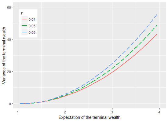
Figure 1. The impact of r on the efficient frontier.

Figure 2 shows how the return rate of the stock $\mu$ influences the efficient frontier. Higher level of the return rate of the stock price $\mu$ lowers the variance of terminal wealth ${\mathrm{Var}}_{t_0,v_0,x_0}\left(X_T^{\ast }\right)$ with the same ${\mathrm{E}}_{t_0,v_0,x_0}\left[X_T^{\ast }\right]$, which is quite clear due to the fact that the investor receives more risk premium as $\mu$ increases and the investor can therefore undertake less risk by investing less into the stock and more into the risk-free asset so as to have the same expected terminal wealth.

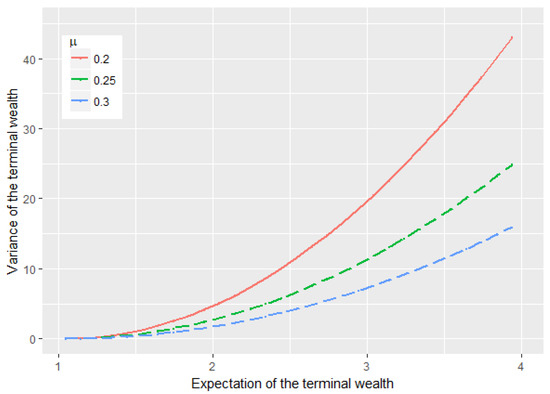
Figure 2. The impact of $\mu$ on the efficient frontier.

The impact of the parameter $\kappa$ on the efficient frontier is presented in Figure 3 below. We see that larger $\kappa$ results in larger ${\mathrm{Var}}_{t_0,v_0,x_0}\left(X_T^{\ast }\right)$ with the same ${\mathrm{E}}_{t_0,v_0,x_0}\left[X_T^{\ast }\right]$. One possible reason is that as $\kappa$ partly stands for the mean-reversion speed of the reciprocal of the stochastic volatility $1/V_t$ (recall the proof of Lemma 3 above), a larger $\kappa$ results in a faster speed of $1/V_t$ towards the long-term level $(\kappa +{\sigma }^2)/\kappa \theta$. Meanwhile, we see that the long-term level is, in fact, decreasing in $\kappa$. These two aspects in turn make the volatility of the stock $V_t$ stays longer around the relatively higher level $\kappa \theta /(\kappa +{\sigma }^2)$. Therefore, the investor has to undertake more risk.

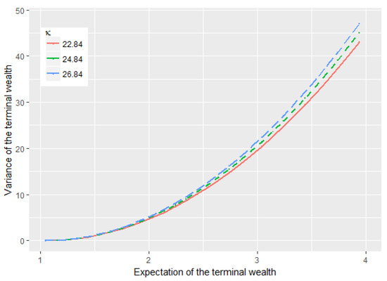
Figure 3. The impact of $\kappa$ on the efficient frontier.

The effect of the parameter $\sigma$ on the efficient frontier is given in Figure 4, which shows that ${\mathrm{Var}}_{t_0,v_0,x_0}\left(X_T^{\ast }\right)$ decreases with the same ${\mathrm{E}}_{t_0,v_0,x_0}\left[X_T^{\ast }\right]$ as $\sigma$ increases. Again, from the proof of Lemma 3 above, we see that $\sigma$ plays a role as the volatility of the reciprocal of volatility process $1/V_t$, and a larger $\sigma$ results in milder movements of the volatility process $V_t$. In addition, we see that the long-run level of volatility $\kappa \theta /(\kappa +{\sigma }^2)$ decreases as $\sigma$ increases. Therefore, these two factors help the investor bear less risk.

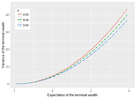
Figure 4. The impact of $\sigma$ on the efficient frontier.

To end this section, we show the dynamics of wealth processes controlled by the statically optimal strategy $u^{\ast }$ (30) and the dynamically optimal strategy $u^{d\ast }$ (33), respectively. By setting 500 equidistant time points over $[0,1]$, we simulate two paths of optimal wealth processes $X_t^{\ast }$ and $X_t^{d\ast }$. Figure 5 illustrates the significant difference between the dynamically optimal wealth process $X_t^{d\ast }$ and the statically optimal wealth process $X_t^{\ast }$. In particular, we see that the result supports the conclusion of Theorem 2 above: the dynamically optimal wealth $X_t^{d\ast }$ is strictly smaller than the expected terminal wealth $\xi =4$ when $t<1$.

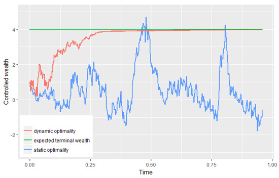
Figure 5. Statically optimal wealth $X_t^{\ast }$ and dynamically optimal wealth $X_t^{d\ast }$.

6. Conclusions

In this paper, a dynamically optimal mean-variance portfolio selection problem within the framework developed in Pedersen and Peskir (2017) in a stochastic environment has been investigated. A 3/2 stochastic volatility model is used to characterize the stochastic volatility of the stock. Considering the methodology in Pedersen and Peskir (2017) to tackle the time-inconsistency of the optimality under mean-variance criterion, we first address the static optimality and solve it by using a general BSDE approach. Under an assumption on model parameters, we obtain the static optimality and the corresponding value function explicitly. By solving the static optimality in an infinitesimally small period of time, the closed-form expression of the dynamic optimality is derived. Considering some technical difficulties, however, we have only studied the case without any state constraint. One branch of research topics in the future is to impose pathwise constraints on the wealth process; see, for example, Pedersen and Peskir (2018).

References

- Ahn, Dong-Hyun, and Bin Gao. 1999. A parametric nonlinear model of term structure dynamics. The Review of Financial Studies 12: 721–62. [Google Scholar] [CrossRef]
- Bakshi, Gurdip, Nengjiu Ju, and Hui Ou-Yang. 2006. Estimation of continuous time models with an application to equity volatility dynamics. Journal of Financial Economics 82: 227–49. [Google Scholar] [CrossRef]
- Basak, Suleyman, and Georgy Chabakauri. 2010. Dynamic mean-variance asset allocation. The Review of Financial Studies 23: 2970–3016. [Google Scholar] [CrossRef]
- Bender, Christian, and Michael Kohlmann. 2000. BSDEs with stochastic Lipschitz condition. Working Paper, Universität Konstanz, Fakultät für Mathematik und Informatik. Available online: http://hdl.handle.net/10419/85163 (accessed on 20 December 2020).
- Bielecki, Tomasz R., Hanqing Jin, Stanley R. Pliska, and Xun Yu Zhou. 2005. Continuous-time mean-variance portfolio selection with bankruptcy prohibition. Mathematical Finance 15: 213–44. [Google Scholar] [CrossRef]
- Björk, Tomas, Mariana Khapko, and Agatha Murgoci. 2017. On time-inconsistent stochastic control in continuous time. Finance and Stochastics 21: 331–60. [Google Scholar] [CrossRef]
- Carr, Peter, and Jian Sun. 2007. A new approach for option pricing under stochastic volatility. Review of Derivatives Research 10: 87–150. [Google Scholar] [CrossRef]
- Chang, Hao. 2015. Dynamic mean-variance portfolio selection with liability and stochastic interest rate. Economic Modelling 51: 172–82. [Google Scholar] [CrossRef]
- Chiu, Mei Choi, and Hoi Ying Wong. 2011. Mean-variance portfolio selection of cointegrated assets. Journal of Economic Dynamics and Control 35: 1369–85. [Google Scholar] [CrossRef]
- Cohen, Samuel N., and Robert James Elliott. 2015. Stochastic Calculus and Applications, 2nd ed. New York: Birkhäuser/Springer. [Google Scholar]
- Cox, John C., Jonathan E. Ingersoll, Jr., and Stephen A. Ross. 1985. A theory of the term structure of interest rates. Econometrica 53: 385–407. [Google Scholar] [CrossRef]
- Drimus, Gabriel G. 2012. Options on realized variance by transform methods: A non-affine stochastic volatility model. Quantitative Finance 12: 1679–94. [Google Scholar] [CrossRef]
- EI Karoui, Nicole, Shige Peng, and Marie Claire Quenez. 1997. Backward stochastic differential equations in finance. Mathematical Finance 7: 1–71. [Google Scholar] [CrossRef]
- Ferland, René, and François Watier. 2010. Mean-variance efficiency with extended CIR interest rates. Applied Stochastic Models in Business and Industry 26: 71–84. [Google Scholar] [CrossRef]
- Han, Bingyan, and Hoi Ying Wong. 2020. Mean–variance portfolio selection under Volterra Heston model. Applied Mathematics and Optimization 2020: 1–28. [Google Scholar] [CrossRef]
- Heston, Steven L. 1993. A closed-form solution for options with stochastic volatility with applications to bond and currency options. The Review of Financial Studies 6: 327–43. [Google Scholar] [CrossRef]
- Hull, John, and Alan White. 1987. The pricing of options on assets with stochastic volatilities. The Journal of Finance 42: 281–300. [Google Scholar] [CrossRef]
- Jones, Christopher S. 2003. The dynamics of stochastic volatility: Evidence from underlying and options markets. Journal of Econometrics 116: 181–224. [Google Scholar] [CrossRef]
- Lewis, Alan L. 2000. Option Valuation under Stochastic Volatility. Newport Beach: Finance Press. [Google Scholar]
- Le Gall, Jean-François. 2016. Brownian Motion, Martingales, and Stochastic Calculus. Berlin and Heidelberg: Springer. [Google Scholar]
- Li, Danping, Ximin Rong, and Hui Zhao. 2015. Time-consistent reinsurance–investment strategy for a mean–variance insurer under stochastic interest rate model and inflation risk. Insurance: Mathematics and Economics 64: 28–44. [Google Scholar] [CrossRef]
- Li, Danping, Yang Shen, and Yan Zeng. 2018. Dynamic derivative-based investment strategy for mean-variance asset-liability management with stochastic volatility. Insurance: Mathematics and Economics 78: 72–86. [Google Scholar] [CrossRef]
- Li, Duan, and Wan-Lung Ng. 2000. Optimal dynamic portfolio selection: Multiperiod mean-variance formulation. Mathematical Finance 10: 387–406. [Google Scholar] [CrossRef]
- Li, Zhongfei, Yan Zeng, and Yongzeng Lai. 2012. Optimal time-consistent investment and reinsurance strategies for insurers under Heston’s SV model. Insurance: Mathematics and Economics 51: 191–203. [Google Scholar] [CrossRef]
- Lim, Andrew E.B., and Xun Yu Zhou. 2002. Mean–variance portfolio selection with random parameters in a complete market. Mathematics of Operations Research 27: 101–20. [Google Scholar] [CrossRef]
- Lin, Xiang, and Yiping Qian. 2016. Time-consistent mean-variance reinsurance-investment strategy for insurers under CEV model. Scandinavian Actuarial Journal 7: 646–671. [Google Scholar] [CrossRef]
- Luenberger, David G. 1968. Optimization by Vector Space Methods. New York: Wiley. [Google Scholar]
- Lv, Siyu, Zhen Wu, and Zhiyong Yu. 2016. Continuous-time mean-variance portfolio selection with random horizon in an incomplete market. Automatica 69: 176–80. [Google Scholar] [CrossRef]
- Markowitz, Harry. 1952. Portfolio selection. The Journal of Finance 7: 77–91. [Google Scholar]
- Pan, Jian, and Qingxian Xiao. 2017. Optimal mean–variance asset-liability management with stochastic interest rates and inflation risks. Mathematical Methods of Operations Research 85: 491–519. [Google Scholar] [CrossRef]
- Pan, Jian, Zujin Zhang, and Xiangying Zhou. 2018. Optimal dynamic mean-variance asset-liability management under the Heston model. Advances in Difference Equations 2018: 258. [Google Scholar] [CrossRef]
- Pedersen, Jesper Lund, and Goran Peskir. 2017. Optimal mean-variance portfolio selection. Mathematics and Financial Economics 11: 137–60. [Google Scholar] [CrossRef]
- Pedersen, Jesper Lund, and Goran Peskir. 2018. Constrained dynamic optimality and binomial terminal wealth. SIAM Journal on Control and Optimization 56: 1342–57. [Google Scholar] [CrossRef]
- Peng, Xingchun, and Fenge Chen. 2020a. Mean-variance asset-liability management with inside information. Communications in Statistics-Theory and Methods 2020: 1–22. [Google Scholar] [CrossRef]
- Peng, Xingchun, and Fenge Chen. 2020b. Mean-variance asset–liability management with partial information and uncertain time horizon. Optimization 2020: 1–28. [Google Scholar] [CrossRef]
- Pliska, Stanley R. 1986. A stochastic calculus model of continuous trading: Optimal portfolios. Mathematics of Operations Research 11: 371–82. [Google Scholar] [CrossRef]
- Shen, Yang. 2015. Mean-variance portfolio selection in a complete market with unbounded random coefficients. Automatica 55: 165–75. [Google Scholar] [CrossRef]
- Shen, Yang. 2020. Effect of variance swap in hedging volatility risk. Risks 8: 70. [Google Scholar] [CrossRef]
- Shen, Yang, and Yan Zeng. 2015. Optimal investment–reinsurance strategy for mean–variance insurers with square-root factor process. Insurance: Mathematics and Economics 62: 118–37. [Google Scholar] [CrossRef]
- Shen, Yang, Xin Zhang, and Tak Kuen Siu. 2014. Mean-variance portfolio selection under a constant elasticity of variance model. Operations Research Letters 42: 337–42. [Google Scholar] [CrossRef]
- Shen, Yang, Jiaqin Wei, and Qian Zhao. 2020. Mean-variance asset-liability management problem under non-Markovian regime-switching models. Applied Mathematics and Optimization 81: 859–97. [Google Scholar] [CrossRef]
- Stein, Elias M., and Jeremy C. Stein. 1991. Stock price distributions with stochastic volatility: An analytic approach. The Review of Financial Studies 4: 727–52. [Google Scholar] [CrossRef]
- Strotz, Robert H. 1956. Myopia and inconsistency in dynamic utility maximization. The Review of Economic Studies 23: 165–80. [Google Scholar] [CrossRef]
- Tian, Yingxu, Junyi Guo, and Zhongyang Sun. 2021. Optimal mean-variance reinsurance in a financial market with stochastic rate of return. Journal of Industrial and Management Optimization 17: 1887–912. [Google Scholar] [CrossRef]
- Yu, Zhiyong. 2013. Continuous-time mean-variance portfolio selection with random horizon. Applied Mathematics and Optimization 68: 333–59. [Google Scholar] [CrossRef]
- Yuen, Chi Hung, Wendong Zheng, and Yue Kuen Kwok. 2015. Pricing exotic discrete variance swaps under the 3/2-stochastic volatility models. Applied Mathematical Finance 22: 421–49. [Google Scholar] [CrossRef]
- Zeng, Xudong, and Michael Taksar. 2013. A stochastic volatility model and optimal portfolio selection. Quantitative Finance 13: 1547–58. [Google Scholar] [CrossRef]
- Zhang, Miao, and Ping Chen. 2016. Mean–variance asset–liability management under constant elasticity of variance process. Insurance: Mathematics and Economics 70: 11–18. [Google Scholar] [CrossRef]
- Zhou, Xun Yu, and Duan Li. 2000. Continuous-time mean-variance portfolio selection: A stochastic LQ framework. Applied Mathematics and Optimization 42: 19–33. [Google Scholar] [CrossRef]
- Zhu, Jiaqi, and Shenghong Li. 2020. Time-consistent investment and reinsurance strategies for mean-variance insurers under stochastic interest Rate and stochastic volatility. Mathematics 8: 2183. [Google Scholar] [CrossRef]
Publisher’s Note: MDPI stays neutral with regard to jurisdictional claims in published maps and institutional affiliations. |
© 2021 by the author. Licensee MDPI, Basel, Switzerland. This article is an open access article distributed under the terms and conditions of the Creative Commons Attribution (CC BY) license (http://creativecommons.org/licenses/by/4.0/).