Article

Assessing the Performance of Random Forests for Modeling Claim Severity in Collision Car Insurance

1
Department Alpine Region Development, Institute for Tourism and Leisure, University of Applied Sciences of the Grisons, Comercialstrasse 19, 7000 Chur, Switzerland
2
Center of Data Analysis, Simulation and Visualization, Department Applied Future Technologies, University of Applied Sciences of the Grisons, Ringstrasse 34, 7000 Chur, Switzerland
3
Department of Actuarial Science, Faculty of Business and Economics (HEC Lausanne), University of Lausanne, Extranef, 1015 Lausanne, Switzerland
4
Swiss Finance Institute, University of Lausanne, 1015 Lausanne, Switzerland
*
Author to whom correspondence should be addressed.
These authors contributed equally to this work.
Risks 2021, 9(3), 53; https://doi.org/10.3390/risks9030053
Submission received: 20 February 2021 / Revised: 8 March 2021 / Accepted: 9 March 2021 / Published: 16 March 2021
(This article belongs to the Special Issue Risks: Feature Papers 2021)

Abstract

:
For calculating non-life insurance premiums, actuaries traditionally rely on separate severity and frequency models using covariates to explain the claims loss exposure. In this paper, we focus on the claim severity. First, we build two reference models, a generalized linear model and a generalized additive model, relying on a log-normal distribution of the severity and including the most significant factors. Thereby, we relate the continuous variables to the response in a nonlinear way. In the second step, we tune two random forest models, one for the claim severity and one for the log-transformed claim severity, where the latter requires a transformation of the predicted results. We compare the prediction performance of the different models using the relative error, the root mean squared error and the goodness-of-lift statistics in combination with goodness-of-fit statistics. In our application, we rely on a dataset of a Swiss collision insurance portfolio covering the loss exposure of the period from 2011 to 2015, and including observations from 81 309 settled claims with a total amount of CHF 184 mio. In the analysis, we use the data from 2011 to 2014 for training and from 2015 for testing. Our results indicate that the use of a log-normal transformation of the severity is not leading to performance gains with random forests. However, random forests with a log-normal transformation are the favorite choice for explaining right-skewed claims. Finally, when considering all indicators, we conclude that the generalized additive model has the best overall performance.

1. Introduction

In the last years, especially in the area of car insurance, many insurers have experienced high fluctuations in their customer portfolio, due to increased competition and the appearance of new technologies (Kamakura et al. 2003). To stay competitive, products must be priced adequately (Bieck et al. 2010; Maas et al. 2008). Traditionally, actuaries rely on linear regression models to calculate the premiums. Such models used explanatory variables, including the characteristics of the policyholder, of the risk insured, and of the contract configuration. Usually, two models are separately calibrated, one for the claim severity and one for the claim frequency (Frees et al. 2016; Ohlsson and Johansson 2010). The pure premium is then obtained by combining both models. In that framework, the severity relates to the average claim amount, while the frequency represents the ratio of the number of claims to the exposure (Bellina 2014; Brisard 2014). Over the last decade, machine learning techniques have won a lot of attention in the area of insurance analytics (Denuit et al. 2019a, 2019b; Quan and Valdez 2018). Machine learning methods are applied in the context of ratemaking (Dalkilic et al. 2009; Huang and Meng 2019; Lowe and Pryor 1996; Pelessoni and Picech 1998; Richman 2018), fraud detection (Li et al. 2018; Wang and Xu 2018), extreme value theory (Velthoen et al. 2021), forecasting (Perla et al. 2020), and in the explanation of the lapse behavior of customers (Guelman et al. 2012; Hu et al. 2020; Staudt and Wagner 2020), among others. While such models are used to select relevant risk factors and automate the creation of categories for continuous variables (Dougherty et al. 1995; Henckaerts et al. 2018), full-pricing applications are scarce, see, e.g., Guelman (2012) and Henckaerts et al. (2020). In claims modeling, most of the current academic research focuses on machine learning methods to develop claim frequency models (Denuit et al. 2020; Ferrario et al. 2018; Noll et al. 2018; Schelldorfer and Wüthrich 2019; Wüthrich and Buser 2018) and much less attention is given to severity modeling (see, e.g., Dewi et al. 2019; Staudt and Wagner 2019).

1.1. Aim and Methodology

In this paper, we focus on insurance claim severity modeling and add insights to the existing body of research (see, e.g., Charpentier 2014, chp. 14, and the literature review below). Our research aims to respond to the following research question: what is the best performing model to model the claim severity in collision car insurance? Driven by our data, we focus on the log-normal distribution assumption which is often used. However, the impact of the distribution assumption on the prediction of damage levels from different models has been given less attention until now. Our objective is to calibrate prediction models for the claim severity and compare the performance of generalized additive models (GAM), generalized linear models (GLM), and random forests (RF). Traditionally, the performance of models is evaluated with the help of goodness-of-fit statistics (GOF). We extend this step by applying goodness-of-lift statistics (GOL), see Denuit et al. (2019). Two reference models are derived, an optimal GAM and a GLM using data-driven binning for continuous covariates following the techniques of Henckaerts et al. (2018). Because the GLM with categorical variables is still the favorite model setup in many insurance companies, it is important for us to measure the performance of the data-driven binning method along GOF and GOL. In the RF setup, we consider two models using the log-transformation of the claims, like in the GLM, and the claim severity without transformation. We compare the performance of these models to the one of the reference models. Our aim is to measure the impact of the log-transformation on the performance of the severity level, i.e., we measure, with the help of GOF and GOL, the performance of the models when back-transforming the log predictions. This back-transformation will be discussed in detail in this paper. We calibrate our models using comprehensive claims data from a Swiss insurer covering 81 309 settled claims. Inn order to measure the prediction performance, we split the data in training and test samples covering the period from 2011 to 2014, respectively, the year 2015.

1.2. Literature on Models and Prediction Performance

GLM introduced by Nelder and Wedderburn (1972) are the “industry standard” to explain the claim severity. In such models, the response variable is distributed according to a distribution of the exponential family (e.g., a Gamma or a log-normal distribution), which is well suited for non-life insurance claims (Ohlsson and Johansson 2010). Traditionally, a log-normal distribution is applied in GLM by log-transforming the dependent variable and then assuming a normal distribution (Frees et al. 2016). While covariates interact as linear predictors in GLM and given that continuous variables rarely interact this way in practice, Hastie and Tibshirani (1990) extend the linear models by relating the response to the continuous variables through a smoothing function in GAM. Because insurers prefer the simplicity of GLM with categorical variables, we use evolutionary trees to derive optimal classes for the continuous variables. The data-driven binning approach closely follows the work of Henckaerts et al. (2018) and Staudt and Wagner (2019). In our procedure, we take particular care in optimizing the number of classes using a penalty function (Grubinger et al. 2014). Following the Bayesian information criteria (BIC), we propose an “optimal” GAM using smoothing functions for the continuous variables and a GLM relying only on categorical variables. While GAM and GLM need a prior variable and interaction selection, this is automated in RF through a specified algorithm. Thus, the interactions that are included in RF models are not limited to a user-specified selection (Hastie et al. 2009; Kuhn and Johnson 2013). Usually, RF models are optimized through the root mean squared error (RMSE) optimization function. However, this optimization function relates to the assumption that the response is normally distributed. Because the claim distribution is right-skewed with only positive values, this assumption is not fulfilled. Hence, we also tune an RF model using the log-transformation used in the regression models. This allows for us to compare the performance among GAM, GLM, and RF models, and to study the impact of the choice of the distribution assumption on the predictions.
While the BIC serves to assess the model performance in GAM and GLM, this function cannot be applied to RF models. Chai and Draxler (2014); Cort and Kenji (2005); Willmott et al. (2009) propose using the RMSE or the mean absolute error (MAE) to assess the performance of machine learning models. Denuit et al. (2019) extend these measures of evaluation and suggest using the area between the concentration and Lorentz curve (ABC) and the integrated concentration curve (ICC). These measures are called GOL statistics and they consider the appropriateness of the predictions, including customers’ claim severity. With the help of the ABC and ICC, we measure the relation between the observed and predicted claim severity (Denuit et al. 2019). On a macro-level, the overall coverage of the total claims by the predictions can be measured with the relative error (RE). In our discussion, we highlight the advantages and disadvantages of the different models. Additionally, we focus on the smoothness of the predictions through contiguous values of the (continuous) risk factors on the individual level. For this purpose, the confidence intervals on the predictions play a major role. However, machine learning and non-parametric models only provide predictions at given points (Khosravi et al. 2011). We build confidence intervals while using the bootstrap method, where new samples are randomly built with replacement and a part of the observations are held out (Carney et al. 2003; Veaux et al. 2014). The so-obtained confidence intervals for the RF model are compared with the ones of the GAM and GLM. We measure the overall prediction performance with the RMSE, MAE, ABC, ICC (individual error), and the RE (overall error).

1.3. Main Results

The main results of our case study are, as follows: in terms of GOL and GOF, GAM is leading to the most appropriate model on the training and test samples. Using a combination of GOL and GOF is bringing enhanced insights in the model interpretation, which GOF alone cannot give. The GLM obtained with the method of Henckaerts et al. (2018) has a good overall performance. However, GAM generates better predictions on the test sample. The log-transformed RF model has a good performance on the right-skewed data, whereas the overall expenses are not covered. The log-transformed RF model shows much lower values for the overall predictions in the violin plot when compared to the other models. The RF model based on a normal distribution assumption covers the total amount of claims well. However, this model is not outperforming other measures. Further, on the selected profiles, RF yields results with low variations along the continuous variables. This helps to explain why RF covers individual claims less well. The log-transformation requires a back-transformation which impacts the performance. Bootstrapping and confidence intervals help to explain the variation of the different factors, so that RF can be an additional asset next to GLM and GAM in practice.
The remainder of the paper is structured, as follows: in Section 2, we describe the available data, analyze the severity distribution, and provide descriptive statistics. In Section 3, we derive the GAM, GLM, and RF models, and then calibrate them on the training data. In Section 4, we describe and discuss the performance of the models on our test sample. We conclude in Section 5.

2. Description of the Dataset

Our study relies on a longitudinal dataset of a Swiss car insurer comprising all closed collision claims that were registered during the period from 2011 to 2015. In Section 2.1, we describe the available data and risk factors. We study the distribution of the claim severity and provide GOF statistics in Section 2.2. We lay out the relative frequencies along the risk factors in Section 2.3.

2.1. Available Data and Variables

We concentrate on the claim severity, as laid out in the Introduction. Because most customers do not declare damage (Denuit and Lang 2004; Klein et al. 2014; Ohlsson and Johansson 2010), no claims are registered for these customers and the number of available observations is typically low, which also explains the limited number of studies (Charpentier 2014, chp. 14). Our data stem from a Swiss collision car insurance portfolio and report the claims that are made by policyholders during the period from 2011 to 2015. A longer history of observations outbalances the disadvantages of the heterogeneity over the years, e.g., varying weather conditions or number of traffic accidents (Denuit and Lang 2004; Denuit et al. 2007). We denote, by S, the claim severity, which is expressed in Swiss francs (CHF). We restrict our study to private policyholders and only consider settled claims in the present work.1 Our full data cover a total of 81 309 claims over five years summing up to CHF 184 mio. In line with the theory of model evaluation, we divide our dataset in a training and a test sample for assessing the prediction performance (Hastie et al. 2009; James et al. 2013; Kuhn and Johnson 2013). Our training data span four calendar years (2011–2014) and they cover 65,950 claims. The test sample consists of the 2015 data and includes 15,359 claims observations. This setup represents, for example, an environment where an insurer uses available data from earlier years (2011–2014) to predict the claim severity for the following period (2015). In terms of financial volume, we consolidate a total claim amount of CHF 149 mio for the training data and CHF 35 mio for the test data.
Table 1 summarizes the available explanatory variables for the process of ratemaking (Frees 2015), i.e., building homogeneous classes of policyholders (see, e.g., Laas et al. 2016; Staudt and Wagner 2018). Most of the factors are determined at the moment of underwriting of the contract (a priori variables, Denuit and Lang 2004; Denuit et al. 2007; Verbelen and Antonio 2016). The age of the policyholder A G , the bonus-malus level B M , the horsepower of the vehicle H P , the value of the car V C , the value of the accessories as a percentage of the car value A P , the age A C , and weight W C of the car, as well as the longitude L O and latitude L A of the policyholder’s main residence are continuous variables. The bonus-malus level, i.e., the percentage factor applied on the gross premium, measures by experience the riskiness of the policyholder and it is reevaluated every year (a posteriori variable, Antonio and Valdez 2012). If a policyholder has a zero claim history, the value drops below 100%. The variables L O and L A , as well as the categorical variables canton CA and language region LR , relate to the policyholder’s residence area. The linguistic regions divide Switzerland into three regions, namely, the German-, French-, and Italian-speaking areas (Lüdi and Werlen 2005). A more detailed segmentation is given by the 26 cantons. Further, the values for L O and L A are derived from combining the postal code and the name of the place of residence. In our work, we code LR and CA with numbers for data confidentiality reasons (see, e.g., the descriptive statistics in Section 2.3 and Figure A1 in the Appendix A). The nationality NA is recorded along eight categories, where the following classes are used by the insurer: Switzerland, France, Germany and Austria, Spain, Portugal, Italy, Eastern Europe, and Turkey, as well as a class for all other countries. The car usage UT is divided along private use with/without irregular or regular commuter route and professional use. The car is described along the body style CS , the car brand CB , and the number of seats NS . To aggregate car brands, we also consider the group that the car brand is associated with CB g and the country of origin of the brand CB c . Car styles CS follow four categories, namely, hatchback and sedan, limousine, convertible, and other. The variable NS encompasses three classes: having less than, exactly, or more than five seats. The insurance deductible ID is considered along four categories, as offered by the insurer: CHF 300, 500, 1000, and 2000 (or more). Finally, the binary variables gender ( G E ), buying the contract online ( I T ), bonus-malus level protection ( B S ), zero-alcohol engagement ( P M ), driving license withdrawal ( D W ), and driving more or less than 10 000 km per year ( D D ) are available.

2.2. Claim Distribution

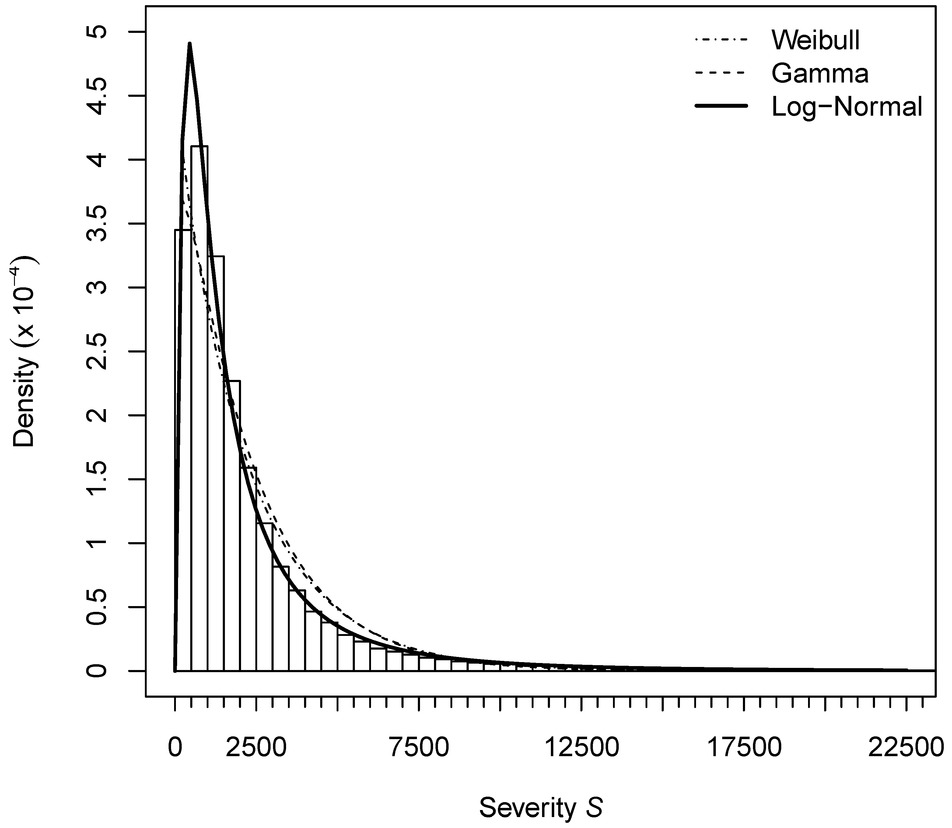
The distribution of the claim severity S is right-skewed (see Figure 1) and it is commonly well described by a Weibull, Gamma, or log-normal distribution (Eling 2014; Ohlsson and Johansson 2010). For choosing the most adequate distribution assumption, we consider three GOF, namely, the Kolmogorov-Smirnov (KS), the Cramer van Mises (CvM), and the BIC measures. Both KS and CvM measures relate to the empirical distribution whereas BIC is linked to the log-likelihood. While the KS measure quantifies the distance between the empirical distribution function of the sample and the cumulative distribution function (Durbin James 1973), CvM extends KS by using the minimum distance estimation (Csorgo and Faraway 1996). The BIC measures the quality of fit (Schwarz 1978). All three measures state that the claim severity S on the training sample is best explained by the log-normal distribution (see Table 2 and Figure 1). In our study, we do not distinguish between the small and large claims and consider all of them together, i.e., we do not split or truncate the dataset, as done in some claim severity models (Albrecher et al. 2017; Denuit and Lang 2004). In collision insurance, and as we only consider settled claims, we do not have as many extremely large claims when compared to other claims data (linked, e.g., to liability insurance). From the graphical illustration, we observe that most of the claims are below CHF 2500 in the training sample. This also holds for the test sample.

2.3. Descriptive Statistics

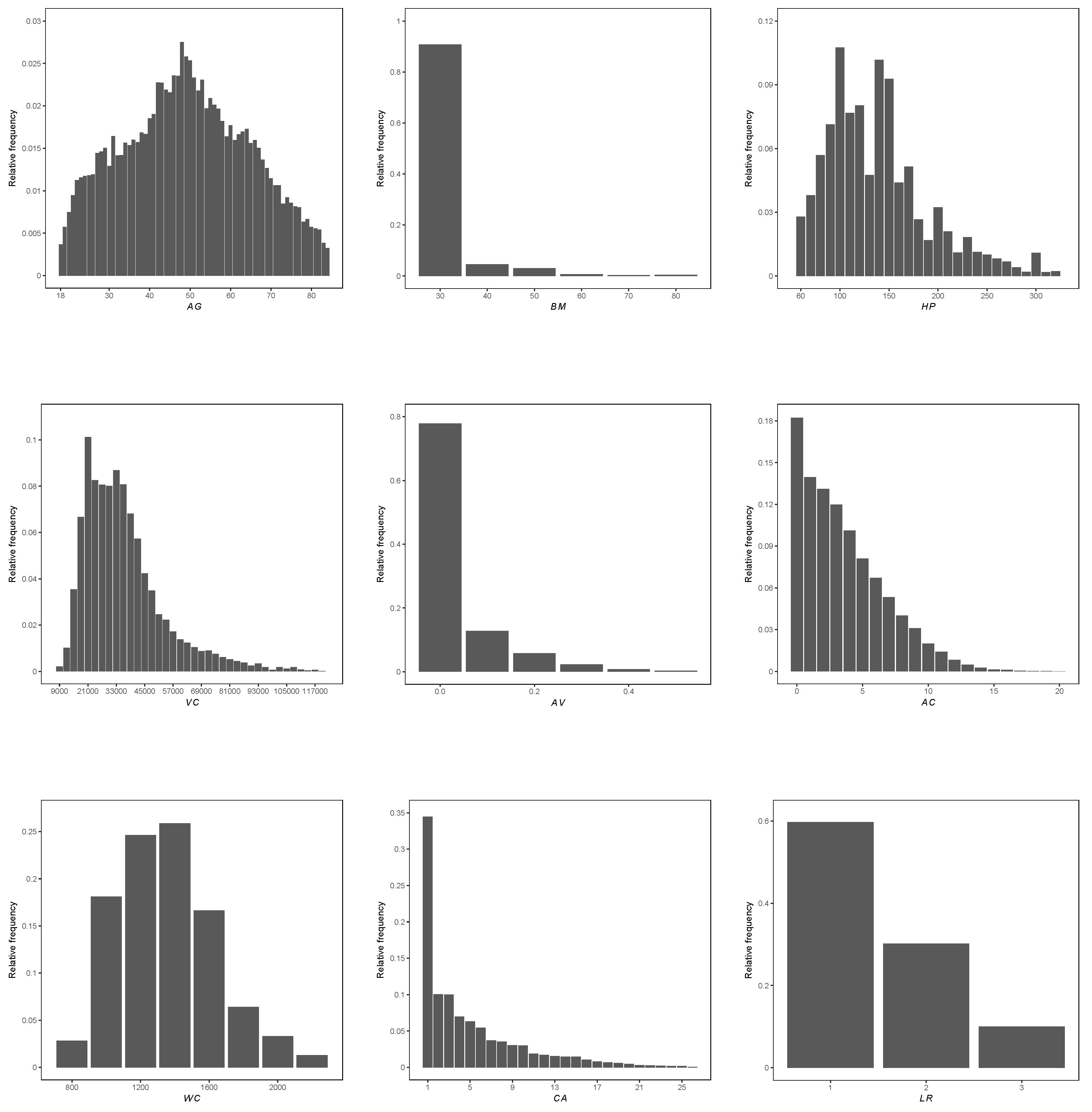
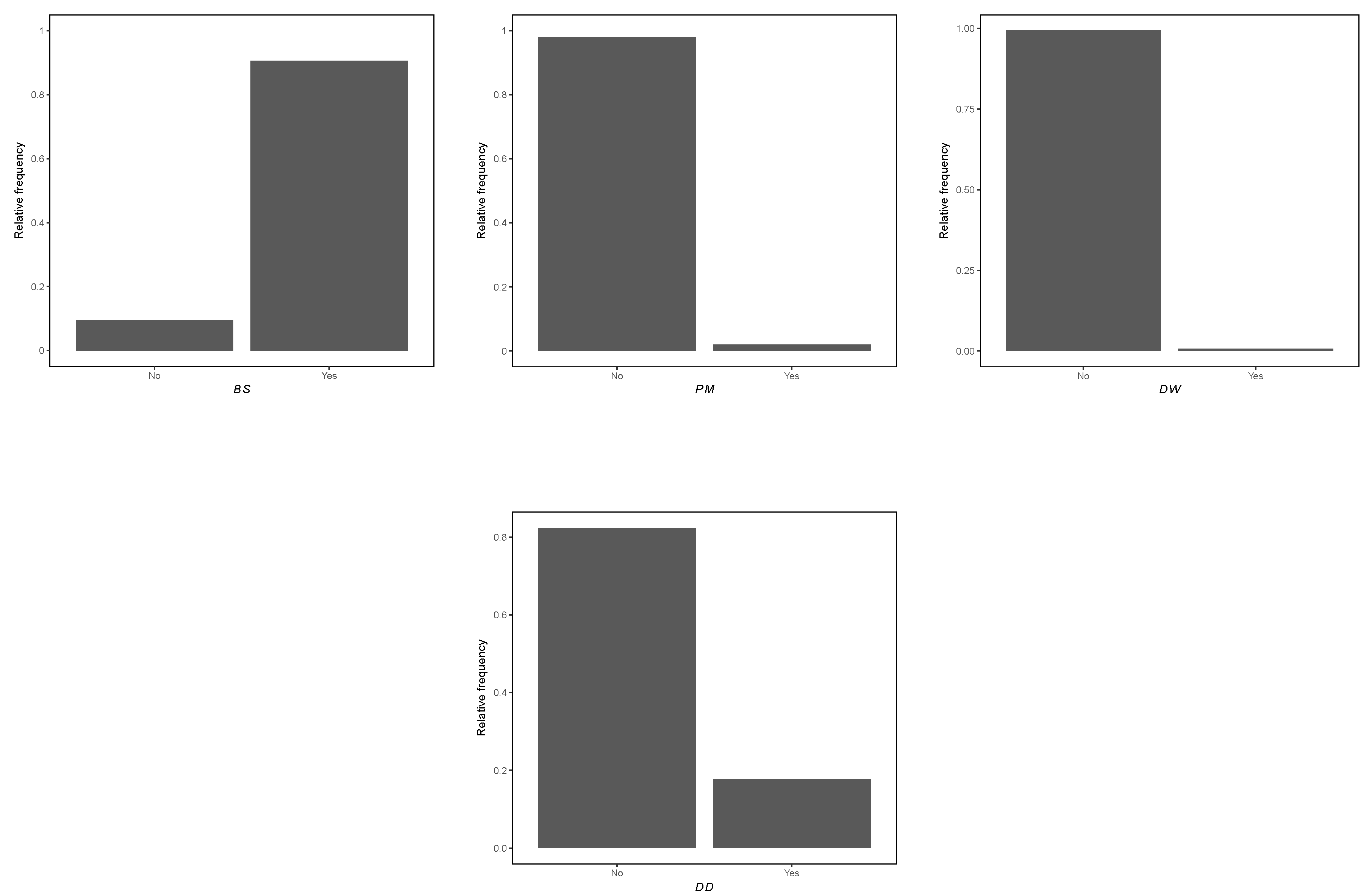
Figure A1 in the Appendix A illustrates the relative frequency of the claim severity S in the training sample along the risk factors. Given the distribution of S along the ages, we note that the quartile values are at 39, 50, and 62 years. Most policyholders (91%) have the lowest bonus-malus level, which means that they pay 30% of the standard premium. The quartiles along the insured vehicles’ horsepower are at the values of 102, 135, and 163. Twenty-five percent of the cars’ values are below CHF 24,800, the median value is CHF 33,900 and the upper quartile CHF 43,720. Most of the insured cars (78%) have accessories that are worth less than 10% of the car value. Half of the policyholders drive rather new cars that are aged below three years. The quartiles in the car weights are 1200, 1400, and 1600 kg. The distribution of the customers along the cantons (numbered from 1 to 26) and language regions (1, 2, 3) shows that the insurer is particularly active in one canton and one language region. Most customers have Swiss nationality (85%) and they use their car solely for private purposes (81%). They are 69% to drive a limousine with five seats (80%). Moreover, the most popular car brand is VW (23%), which originates from Germany (39%) and it is a member of the group VW. The second-largest car band group is PSA (16%), and it includes the major brands Peugeot, Citroën and Opel. This group contains cars with origins of France and Germany. Most cars are produced in Germany, followed by Japan. The insurance deductible is CHF 300 for 80% of the portfolio. Men are responsible for two-thirds (65%) of the claims. Most contracts are not underwritten online (98%) and they include a bonus-malus level protection (91%). Most of the policyholders do not take the zero-alcohol engagement (98%). Nevertheless, they have no driving license withdrawal (99%) and drive more than 10,000 km per year (82%).

3. Model Parameterization

In this section, we link the claim severity S to the risk factors laid out above. First, we derive optimal GAM and GLM under the BIC (see Section 3.1) following Henckaerts et al. (2018) and Staudt and Wagner (2019). Second, we use RF to model S and log S by considering the R M S E as an optimization function (Section 3.2).

3.1. Optimal Regression Models (GAM and GLM)

From the GOF statistics that are provided in Table 2, we observe that the claim severity S is best approximated by a log-normal distribution. This distribution relates to the exponential family, namely to the normal distribution, by log-transforming S. In the following, we use the identity linear link function in a GAM and consider the risk factors that are summarized in Table 1 in a forward and backward stepwise selection procedure. Thereby, the BIC provides a measure for the model performance. The BIC penalty is more severe then, e.g., the Akaike Information Criterion, and will, therefore, favor less complex models. We rely on the BIC, since we aim to retain well-performing models that are as simple as possible. In the GAM, continuous variables are included through a smoothing function and the spatial longitude and latitude information is integrated through an interaction term (Denuit and Lang 2004; Klein et al. 2014). At this stage, we do not consider further interactions between the other risk factors. Both forward and backward stepwise selection processes lead to the following model:
E ( log ( S ) ) = β 0 + β 1 · B S + β 2 · CS + β 3 · CB g + β 4 · ID + f 1 ( A G ) + f 2 ( H P ) + f 3 ( A C ) + f 4 ( W C ) + f 5 ( L O , L A ) .
The selected model only retains 10 of the 25 available explanatory variables. One binary variable, the bonus-malus level protection B S , is included in the model. Three categorical variables are included. They are the car body style CS with four categories, the car brand group CB g with 17 categories, and the insurance deductible ID with four categories. The continuous variables age of the policyholder A G , horsepower of the car H P , age A C , and weight W C of the car are considered through the smoothing functions f 1 to f 4 . Spatial information on the policyholder’s main residence enters through a smoothing function on the interaction between the longitude and latitude in f 5 ( L O , L A ) . The other variables are excluded, since they do not improve the model under the BIC. When applying the model (1) on the data from the training sample, the values of the regression coefficients and the estimated degrees of freedom are reported in the first column of Table A1 in the Appendix A. The estimated degrees of freedom that are related to the smoothing functions correspond to the number of knots of the spline, where a higher degree relates to a higher number of inflection points. For example, for the age of the policyholder f ^ 1 ( A G ) , we find a value of 7.009 , which is higher than for the variables H P , A C , and W C (see Figure 2 for a graphical illustration). The weight of the car variable has an estimated degree of freedom in f ^ 4 ( W C ) that is almost equal to one ( 1.002 ), indicating a quasilinear impact of W C on the response. Further, we observe that most regression coefficients (upper part of Table A1) yield high significance levels (p-values that are below 0.001) with only few sub-categories of the car brand group CB g not being significant. In the following, we test all interactions between the continuous variables A G , H P , A C , and W C , omitting the other (categorical, binary and spatial) factors as they would lead to more complex but not more explicit models. We do not consider the common age-gender interaction, since the gender variable is excluded from the model following the BIC. We find that none of the studied interaction terms improve the model under the BIC and we remain with the GAM that is given in Equation (1).
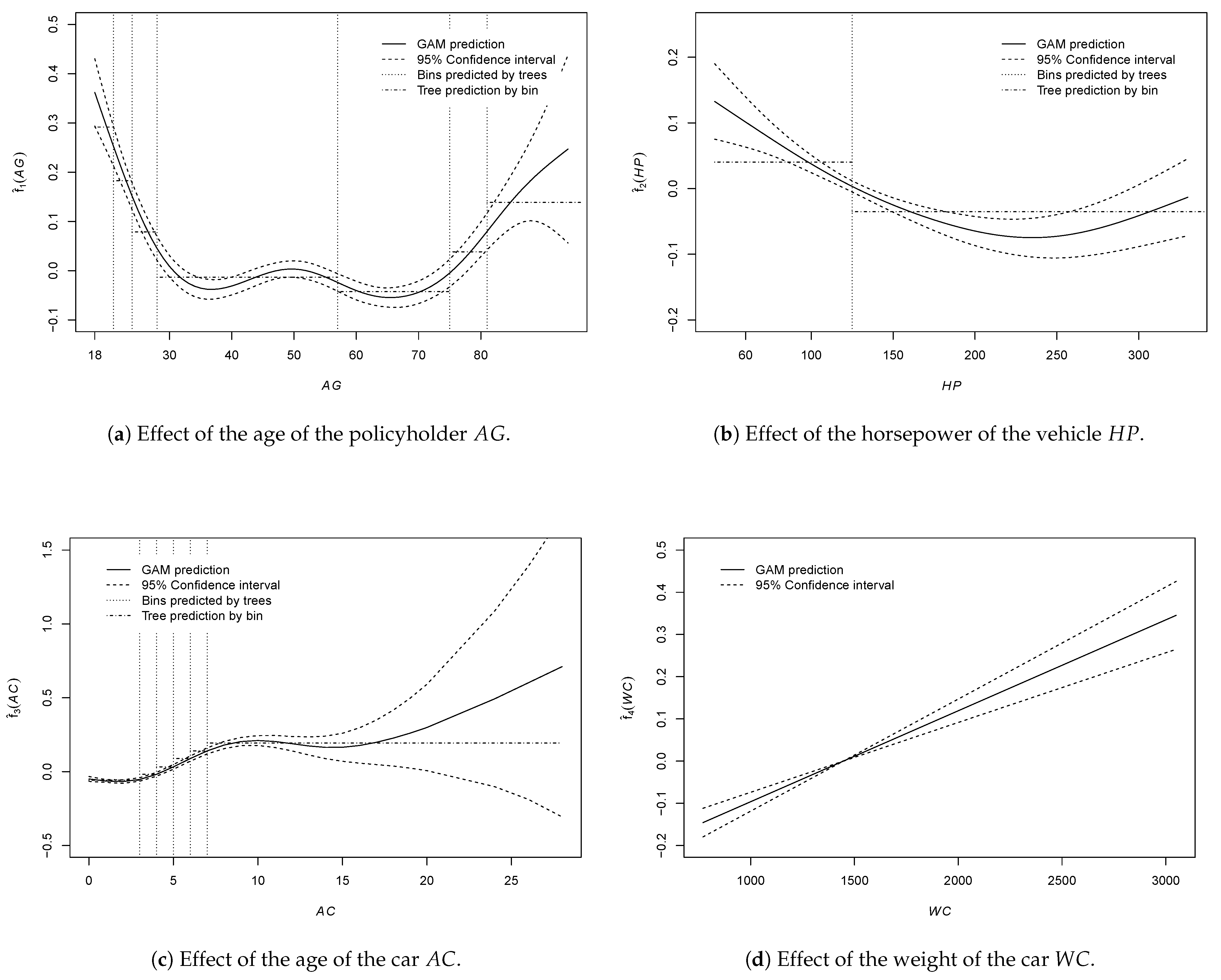
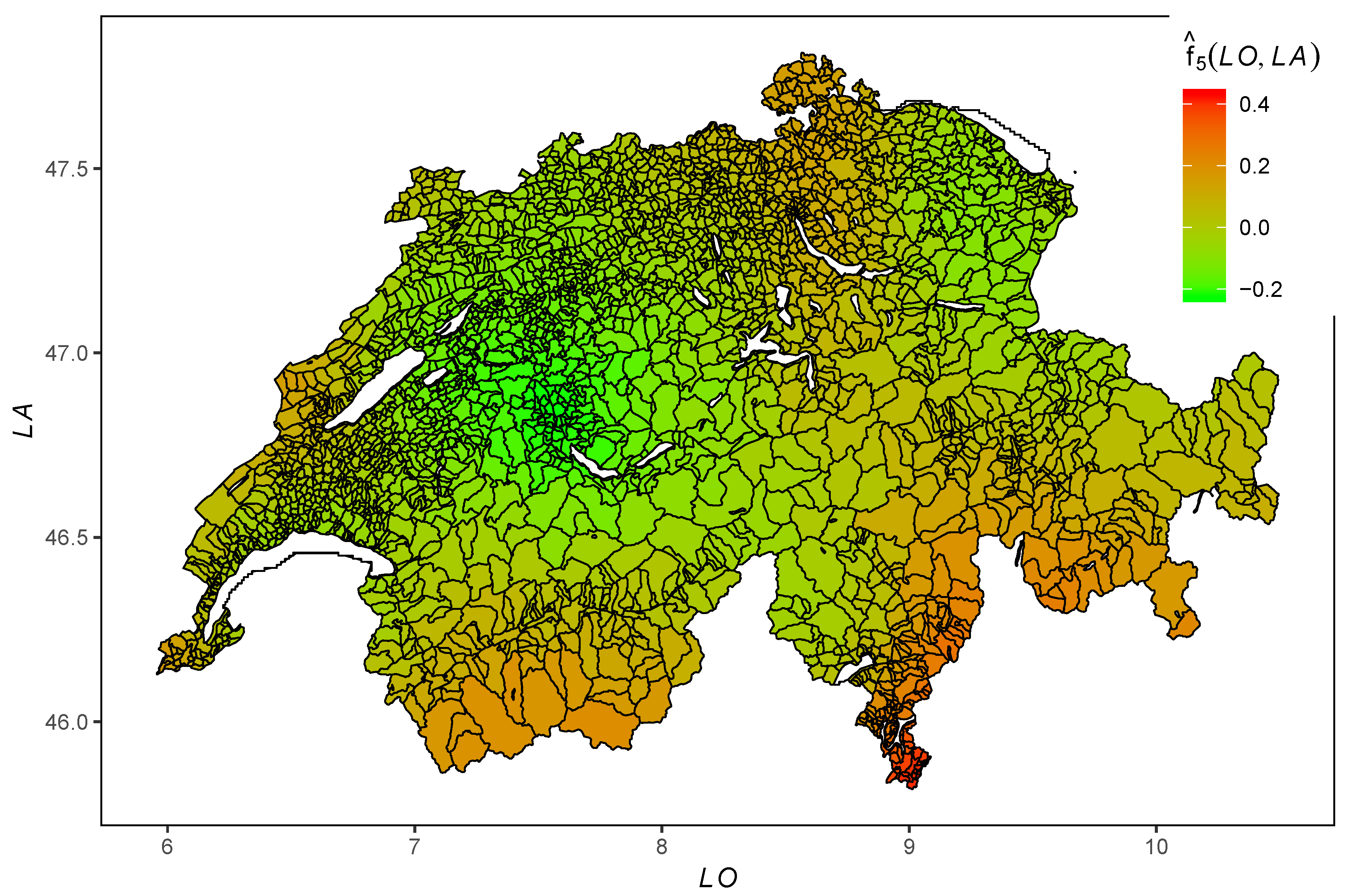
In Figure 2, we illustrate the effects of the continuous variables through the fitted smoothing functions f ^ 1 ( A G ) , f ^ 2 ( H P ) , f ^ 3 ( A C ) , and f ^ 4 ( W C ) . The dashed lines indicate the 95% confidence interval. We observe larger intervals, for example, at higher policyholder ages, where the number of observations is lower. In graph (a), f ^ 1 indicates a higher effect for young customers, which relates to higher claim severity in that customer segment. This effect is decreasing through the age from 18 to 35 years, and they behave non-monotonically in the range between 35 and 75 years. From 75 years on, the effect on the claim severity increases again. Conversely, the smoothing function of the horsepower f ^ 2 that is illustrated in the graph (b) is decreasing for values from 50 to 250 and then increasing. The age of the car effect f ^ 3 ( A C ) in graph (c) is rather constant from zero to three, increasing from three to seven, and finally becoming non-monotonic. As mentioned earlier, the effect of the weight of the car W C is rather linear (graph d). Further, we illustrate the spatial effect f ^ 5 ( L O , L A ) in Figure 3. Customers living in the Italian-speaking region have the highest effect with f ^ 5 ( L O , L A ) = 0.4 , which corresponds to, on average, approximatively 40% more severe accidents than in regions with the baseline (zero) effect. Customers living in the region of the cities of Bern and St. Gallen have values of f ^ 5 ( L O , L A ) = 0.2 . We observe that the effect is increasing from 0.2 to 0.0 when moving from both cities to more rural and remote regions (e.g., Bernese Oberland and Appenzellerland). This indicates that the sole canton information commonly used today can be significantly enriched by integrating more detailed spatial information.
We cannot apply a linear model on these variables, as we observe nonlinear effects for the continuous variables A G , H P , and A C , as well as for the spatial information ( L O , L A ) . From the continuous factors, only the effect of W C is suitable for linear modeling. To build an optimal GLM model, we use a data-driven method to classify the continuous variables A G , H P , and A C into categories. In fact, evolutionary trees can help to bin consecutive values and such a method is, e.g., available in the package evtree in R . We optimize the evolutionary trees through a tuning parameter α in the following penalty function,
n · log ( M S E ) + 4 · α · ( l + 1 ) · log ( n ) ,
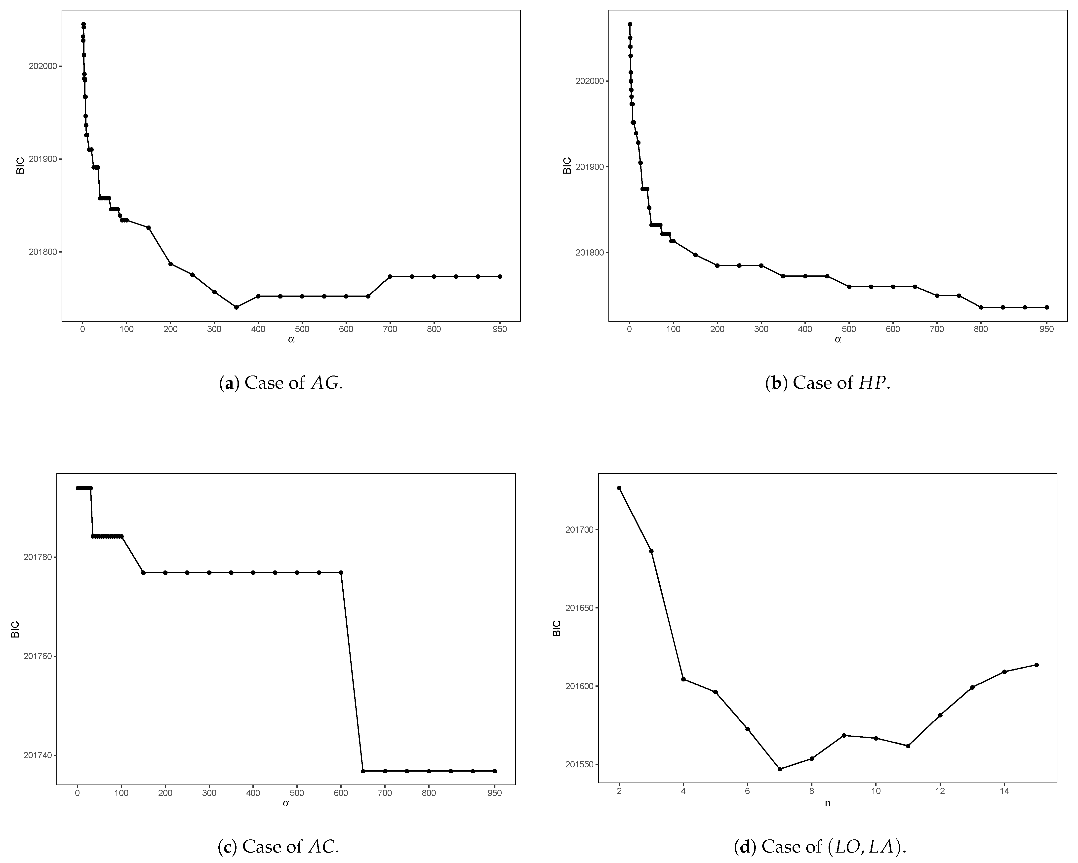
where n relates to the size of the dataset and l is the number of classes. The number of classes l is decreasing with increasing α (Grubinger et al. 2014). This performance function is used to compare the models between each other. The model with the lowest value is considered the best one. However, the penalty (2) decreases with increasing α and it relates to simpler trees. The penalty measure will always choose the simplest model, which, following actuarial experience, is not necessarily the best model (Henckaerts et al. 2018). Thus, we cannot determine the optimal number of classes while exclusively using the penalty function (2) and we propose considering another way to determine the number of classes. At each step, for a given α , we replace one smoothing function f i in Equation (1) by the obtained classes and hold the other variables fixed while determining the performance of the model using the BIC. This allows for us to assess the tradeoff between accuracy and complexity along the classes used. We choose the tuning parameter α out of the set { 1 , 1.5 , 2 , , 9.5 , 10 , 15 , 20 , , 95 , 100 , 150 , 200 , , 950 } . Figure 4 presents the values of the BIC for each α . From graph (a), we read that, for A G , the BIC decreases until α takes the value of 350 and is increasing for higher values of α . Thus, we use α = 350 for deriving the classes for A G . In the case of H P and A C , the BIC decreases with α (see graphs b and c). In both cases, we remain with α = 950 , leading to the simplest model.2 The classes that were obtained for A G , H P , and A C are illustrated in the graphs (a) to (c) in Figure 2 with vertical lines indicating the boundaries of the bins. The dashed-pointed horizontal lines in the graphs indicate the predicted mean effects for each class. Following the above optimization of the penalization parameter, we find that the age of the policyholder is binned into seven classes AG c , the horsepower of the car into two classes HP c , and the age of the car into six classes AC c .
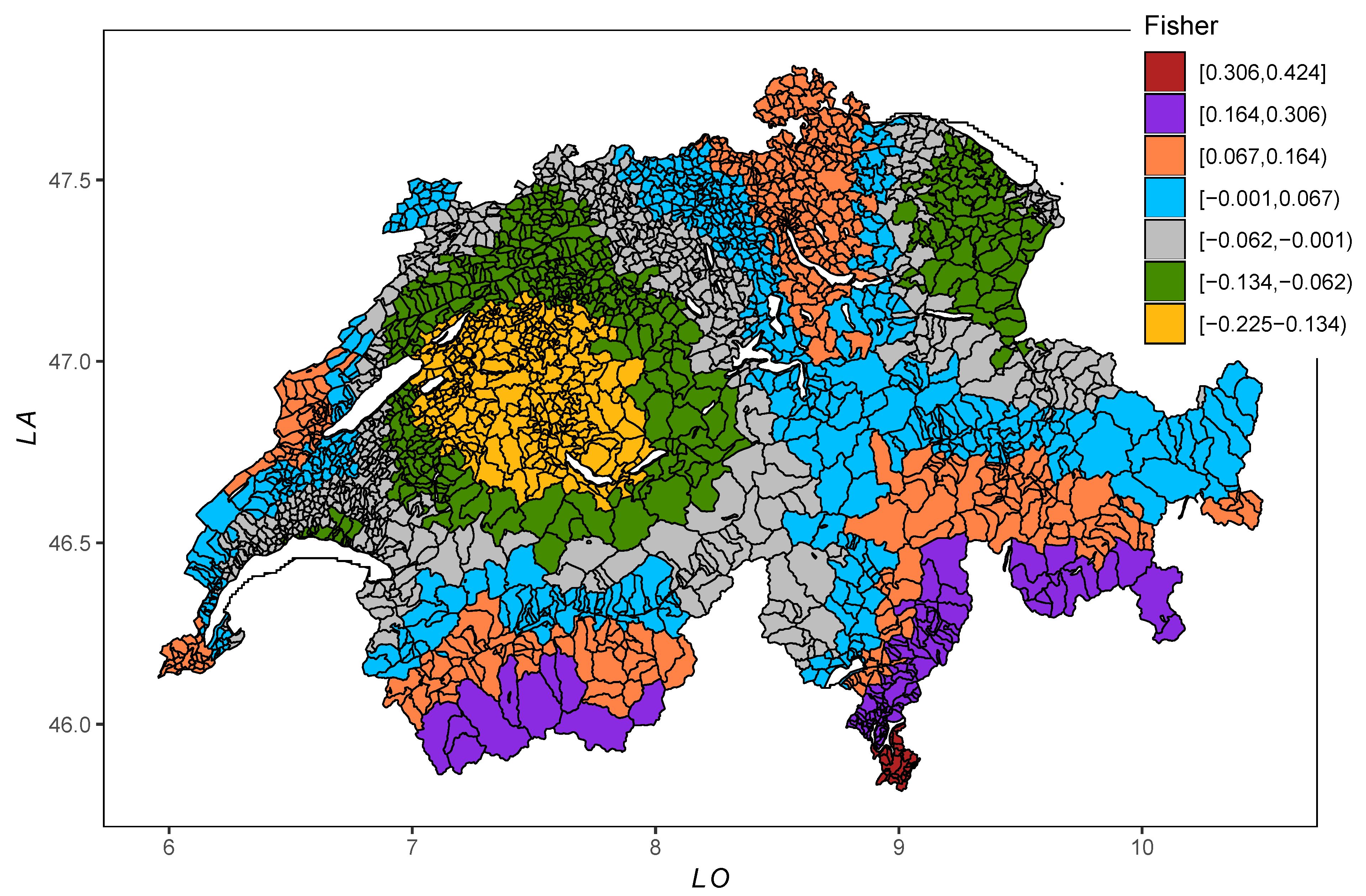
From Figure 3, we observe that there are regions with similar effects on the claim severity. We do not only bin consecutive municipalities but aim to group regions with similar effects’ levels. The evolutionary tree method cannot be applied in this setup and we follow Henckaerts et al. (2018) who propose Fisher’s natural breaks algorithm. This algorithm maximizes the homogeneity within bins by classifying the variables that are close to their calculated average (Slocum et al. 2005). The method is readily available, e.g., in the classInt package in R . The measures evaluating the performance of the created bins suffer from the same problem as the complexity measure shown in Equation (2). Thus, the best number of bins n is chosen by consistently measuring the final BIC performance. We let the parameter n take values between 2 and 15. The best classification (lowest BIC) is obtained while using seven spatial groups ( LO , LA ) c , as can be seen from Figure 4d. Figure 5 presents the regional categories obtained.
While applying the above categories for the continuous variables, we derive the following GLM:
E ( log ( S ) ) = β 0 + β 1 · B S + β 2 · CS + β 3 · CB g + β 4 · ID + β 5 · AG c + β 6 · HP c + β 7 · AC c + β 8 · W C + β 9 · ( LO , LA ) c
The second column in Table A1 reports the regression results.

3.2. Random Forests Models

In the following, we optimally calibrate a RF model on the training sample. Traditionally, the R M S E optimization function is used (Hastie et al. 2009; Kuhn and Johnson 2013). However, this optimization function relies on the assumption that the claim severity S is normally distributed (Chai and Draxler 2014; Willmott et al. 2009). Because, from the GOF statistics in Table 2, we have concluded that S is best described through a log-normal distribution. Considering the log-transform of S, then log S is normally distributed and the R M S E can be applied. In this section, we propose tuning two RF models, one taking log S (denoted by RF log S ) and one taking S as the dependent variable (denoted RF S ). In the numerical implementation, we use the available packages ranger and caret in R .
A RF model is an aggregation of B regression trees, where each tree is built on a bootstrapped sample. While, for each feature/split, a sub-sample of m risk factors is chosen (Hastie et al. 2009; James et al. 2013). Each tree in the optimization is influenced by the node size. To balance the model between accuracy and complexity, we test five different minimum node sizes. Hence, three tuning parameters B, m, and the minimum node size need to be determined.
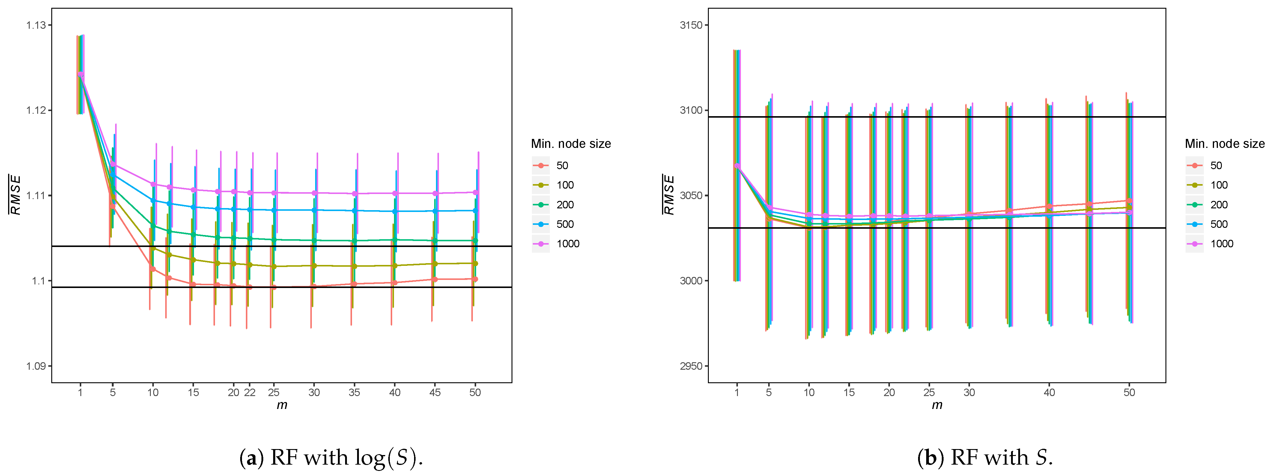
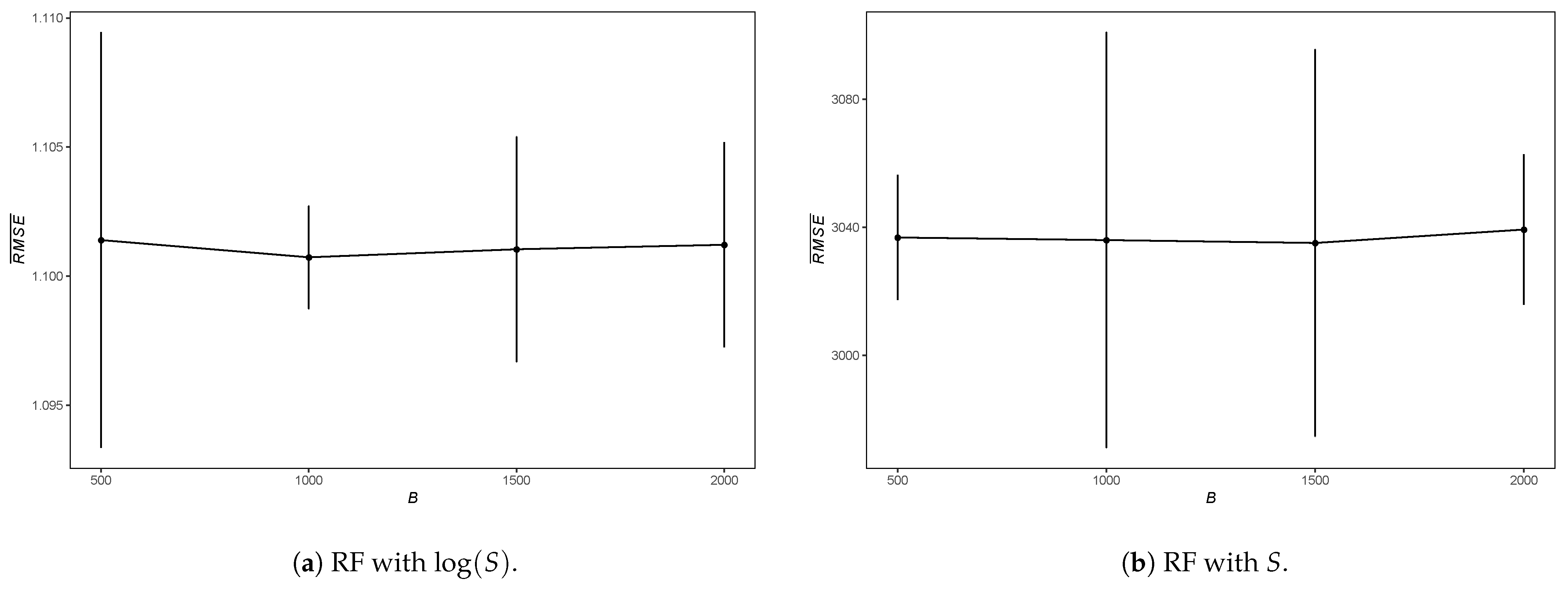
In a first step, we fix B = 1000 and proceed with the choice of the optimal values for m and the minimum node size. We choose m within the set {1, 5, 10, 12, 15, 18, 20, 22, 25, 30, 35, 40, 45, 50} and the minimum node size is fixed to either 50, 100, 200, 500, or 1000 data points in each end node. We use a fivefold cross-validation to determine the best tuning parameters. This can be automatized with the train function in the caret package in R (Kuhn 2008). In a fivefold cross-validation, the training sample is divided into five equally sized random sub-samples (without replacement). Four sub-samples of the five are used for training the model and the last one is used for validating the model (the validation sample, James et al. 2013; Kuhn and Johnson 2013). The performance of the model on the validation sample is measured with the help of the R M S E . The results that are illustrated in Figure 6 report the average value of the fivefold cross-validation samples’ R M S E , denoted by R M S E ¯ , with the related standard errors s e for different values of m. The 95%-confidence intervals are calculated as R M S E ¯ ± 1.96 · s e (Nicholls 2014). In order to choose the best model, we remain with the simplest model having the lowest R M S E ¯ within the 95%-confidence interval of the best model. In the case of RF log S , the best results are obtained using m = 25 and a minimum node size of 50. We retain the parameter value of m = 10 and a minimum node size of 50, yielding a simpler model within the 95% confidence interval of the best model (solid horizontal lines in Figure 6). Figure 6b illustrates the results for RF S . We observe a minimum error for m = 10 when the minimum node size equals 50, and we retain the values of m = 5 and a minimum node size of 50 for further modeling. We note that a model with m = 1 (one risk factor per regression) is still within the confidence interval of the RF S model, but we exclude such a simple model. We are aware of the limitations of the tuning grid and the related results. We limited the tuning grid due to the available computational resources of the authors at the time of writing.
In a second step, we adjust for the optimal number of trees B with the above values for m and minimum node size. Using again fivefold cross-validation, we test the values of B = 500 , 1000, 1500, and 2000. While no important influence can be observed in both RF models (see Figure 7), we remain with B = 1000 . Thus, the RF log S model is parameterized with B = 1000 , m = 10 and a minimum node size of 50 and RF S uses the parameters B = 1000 , m = 5 and minimum node size of 50.

4. Comparison and Discussion of the Models

In this section, we compare the performance of the GAM (Equation (1)), GLM (Equation (3)), and both RF models. Because three of the models are based on log S , we consider the back-transformation to S ^ for the prediction of S. First, we make an overall comparison of the models while using different statistical measures. Second, for selected individual profiles, we focus on the smoothness of the predictions through contiguous values of the continuous risk factors.

4.1. Overall Model Comparison

For comparing the models, we take different perspectives and consider measures from the GOF (Willmott et al. 2009) and GOL (Denuit et al. 2019) statistics on the training and test samples. From the GOF statistics, we use the root mean squared error (RMSE), the mean absolute error (MAE), and the total relative error (RE). The total relative error evaluates the deviance of the prediction from the total claims amount, as follows:
R E = i ( S i S ^ i ) i S i .
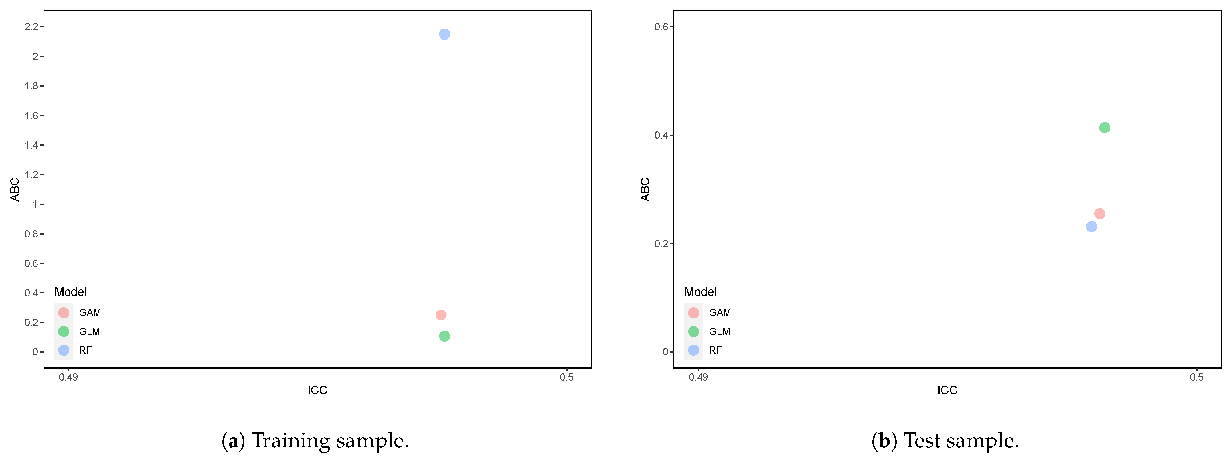
Two GOL statistics are applied, namely the area between the concentration and Lorentz curve (ABC) and the integrated concentration curve (ICC). The concentration curve measures the share of true premiums that should have been collected for the portfolio, whereas the Lorentz curve measures the share of premiums that were collected for the portfolio. The smaller the area between both curves, the better the model in terms of premium income needs. The same interpretation holds for the ICC. Denuit et al. (2019) choose the optimal model by considering the combination of the lowest ABC and ICC. Further, we consider violin plots and the effective model predictions to waluate the models.
As we have log-transformed the claim severity S in the GAM, GLM, and RF log S model, we transform the predictions from the log ( log S ^ ) to the claim severity level ( S ^ ). By exponentiating the predictions exp ( log S ^ ) , we lose some properties of the data (Longford 2009). Indeed, the sampling variance σ needs to be included. Because traditional back-transformation methods can result in poor predictions, we use the non-parametric method described in the paper of Duan (1983),
S i ^ = exp log S i ^ · 1 n j = 1 n exp ϵ ^ j ,
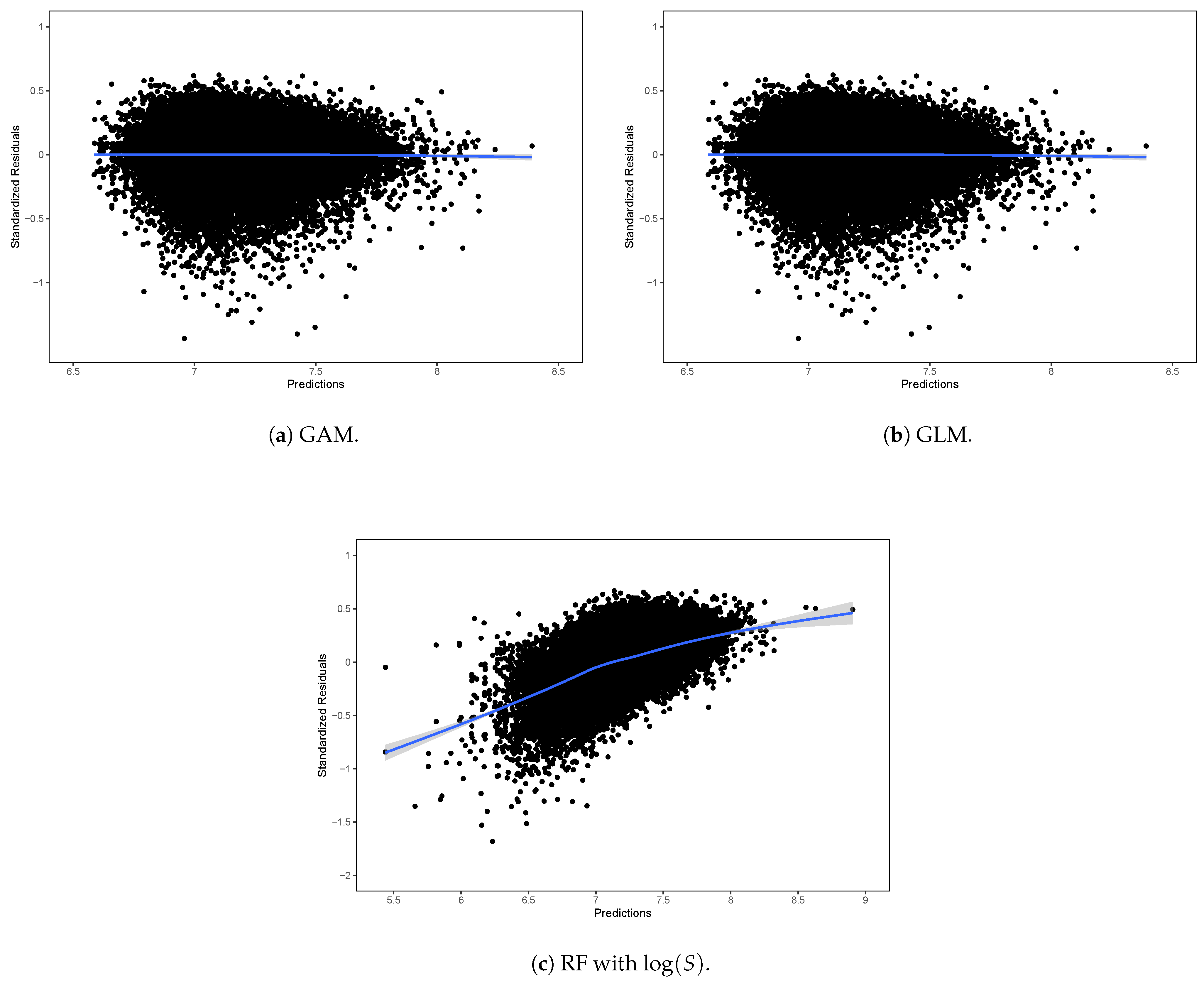
where n denotes the size of the dataset and ϵ ^ j the residuals linked to the observation j. Duan’s smearing estimator demands that the error is homoscedastic (Ai and Norton 2000; Manning 1998; Manning and Mullahy 2001). The homogeneity in variance is traditionally controlled by representing the standardized residuals against the predictions. The homoscedasticity is given when the predictions are independent from the residuals, which means whether the points are randomly distributed along the standardized residuals and the predictions. We add a cubic spline estimator to the error visualizations of GAM, GLM, and RF log S (see Figure 8) to test whether the distribution of the errors is homoscedastic. GAM and GLM residuals are homoscedastic, as the cubic spline is a line, which indicates that the homogeneity of the variance is given. However, R F log S standardized residuals against the predictions show a positive trend that we relate to heteroscedastic errors. Here, the smearing estimator from Duan (1983) is biased. Following Ai and Norton (2000), we replace the residuals by the standardized residuals in Equation (5), i.e.,
S i ^ = exp log S i ^ · 1 n j = 1 n exp r j 1 n 1 j = 1 n ( r j r ¯ ) · r ¯ ,
where r i is the residual of the ith observation and r ¯ is the residual average. In conclusion, we use Equation (5) to transform the predictions from the GAM and GLM, while Equation (6) is used in the case of RF log S .
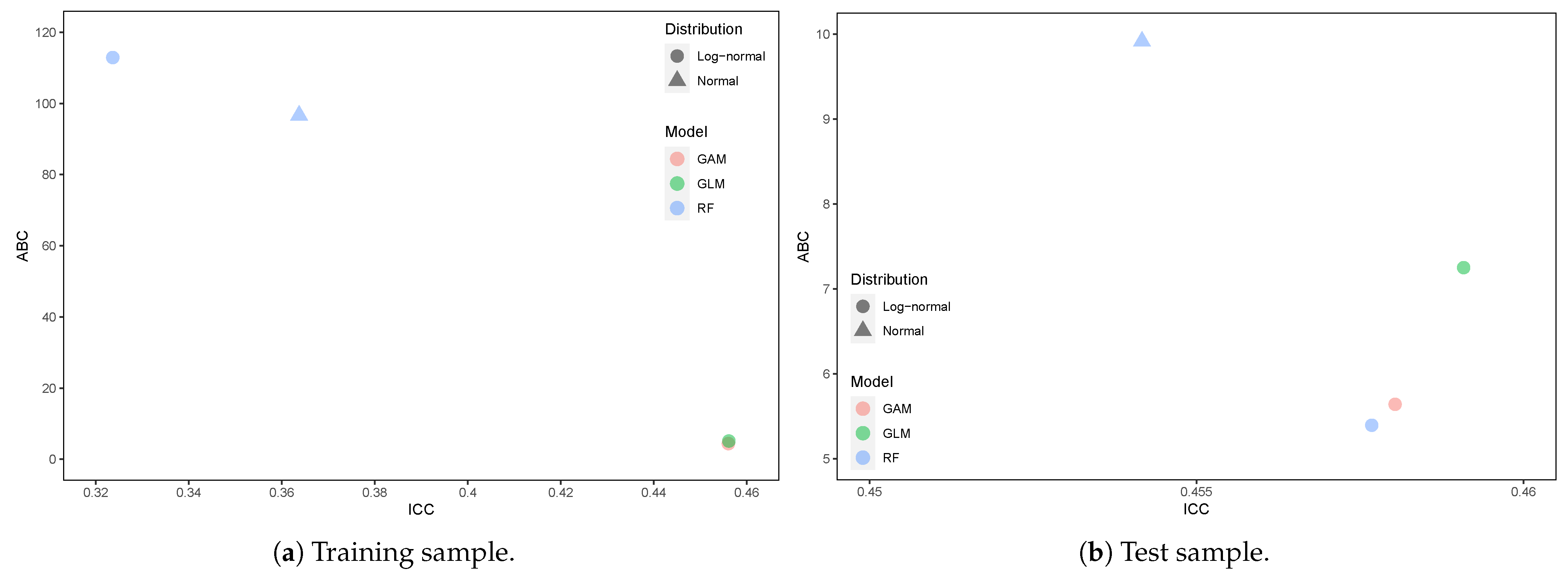
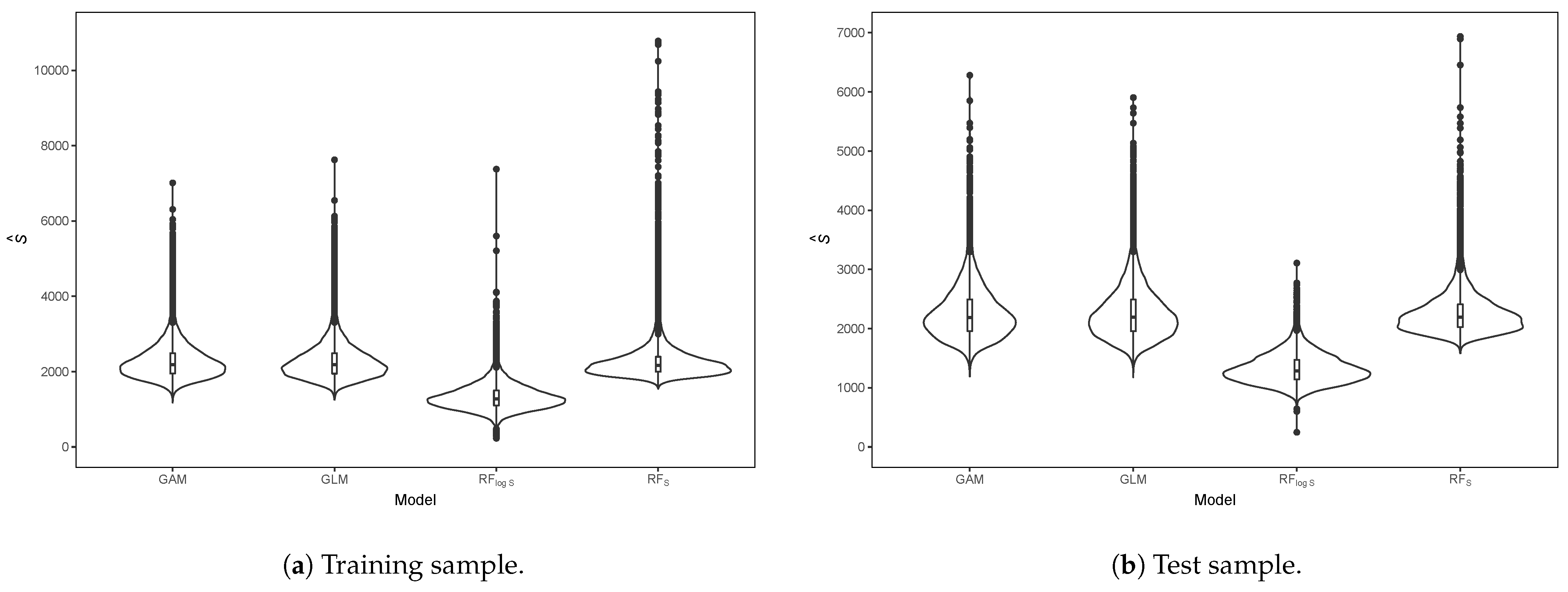
We report the GOL and GOF results for the training sample in Table 3, and for the test sample shown in Table 4. We observe that no model outperforms all others throughout the different. We observe that the RF S has the smallest RE and RMSE value on the training sample. The RF S model leading to the lowest RMSE was expected, as the model is optimized along this specific optimization function. For the other models, no important differences are found in the RMSE. Further, RF log S has the lowest MAE, but, at the same time, the largest deviation from the total sum of claims (RE of 41.4%). Both of the RF models have high ABC values. A large ABC means that the RF models do not cover the individual claims. At the same time, these models have the smallest ICC, which means that the models cover the expected share of true premiums in the portfolio. By taking the combination of ABC and ICC, as described by Denuit et al. (2019), see Figure 9a, GAM is the best model. The violin plots in Figure 10a represent similar density plots for GAM and GLM. The violin plot of RF S has a wider body and a similar median value than GAM and GLM. However, the one for RF S has much more extreme predictions, better matching the larger claims. The RF log S has a similar density plot than RF S , but with much lower values and not as high predictions as the other models. This explains why RF log S has such a high RE, which indicates that this model is not well overlapping the total exposure of the portfolio. This is in accordance with the ABC, which tells us that the predictions do not cover the claim severity of the portfolio. The low MAE and ICC confirm that RF log S is especially well performing on the lower part of the claims, which is due to the right-skewed data. The RF S model has a much better coverage for the total exposure. Overall, the GAM performs well throughout all measures, with no extremely bad outcomes, and one can consider GAM to be the preferred model on the training sample.
Because such models are used in practice to evaluate the premiums for the following year, we focus now our study to see how the four models perform on unseen data. On the test sample, see Table 4, GLM covers the total sum of claims best. The deviation of the RF log S model in terms of total claims is very high. The RF S model remains with the lowest RMSE, closely followed by the GAM and GLM. The RF log S model conforms best with the lowest MAE, i.e., it has on average the best cover of the claims. By considering the combination of ABC and ICC, see Figure 9b, GAM and RF log S are similarly positioned. This means that GAM and RF log S are best covering the portfolio expenses and the expected true premium. The violin plots, Figure 10b shows that RF log S has much lower predictions when compared to the alternatives. The MAE and ABC measures confirm that the RF log S model is well covering the right-skewed data, but it comes with issues in the higher claims. For the other models, we observe similar behaviors when considering the median. We note that the RF S model yields higher predictions. When considering ABC, RF S is less well covering the portfolio needs. Considering the test sample GAM and RF log S seems to be the best alternatives. By combining the discussion from both training and test samples, an actuary would probably remain with the GAM model.
We analyze, in Table 5, if these differences remain on the log scale, as we observe high discrepancies for large claims in the RF log S model. Therefore, we report the RMSE, MAE, ABC, and ICC measures. We observe no relevant differences in the RMSE, MAE, and ICC for the training sample. The only difference is observed in ABC, where the GLM is performing better and RF the worst. By considering the combination of ABC and ICC, see Figure 11a, the GLM is the best model in the training setup. When considering the results of the test sample, we do not measure the differences in the RMSE, MAE, and ICC. In the case of the ABC, GLM is worse than the alternatives. When considering Figure 11b GAM and RF log S have similar results for ABC and ICC. This hints that the RF model and GAM can better generalize predictions when compared to the GLM.

4.2. Comparison on Individual Profiles

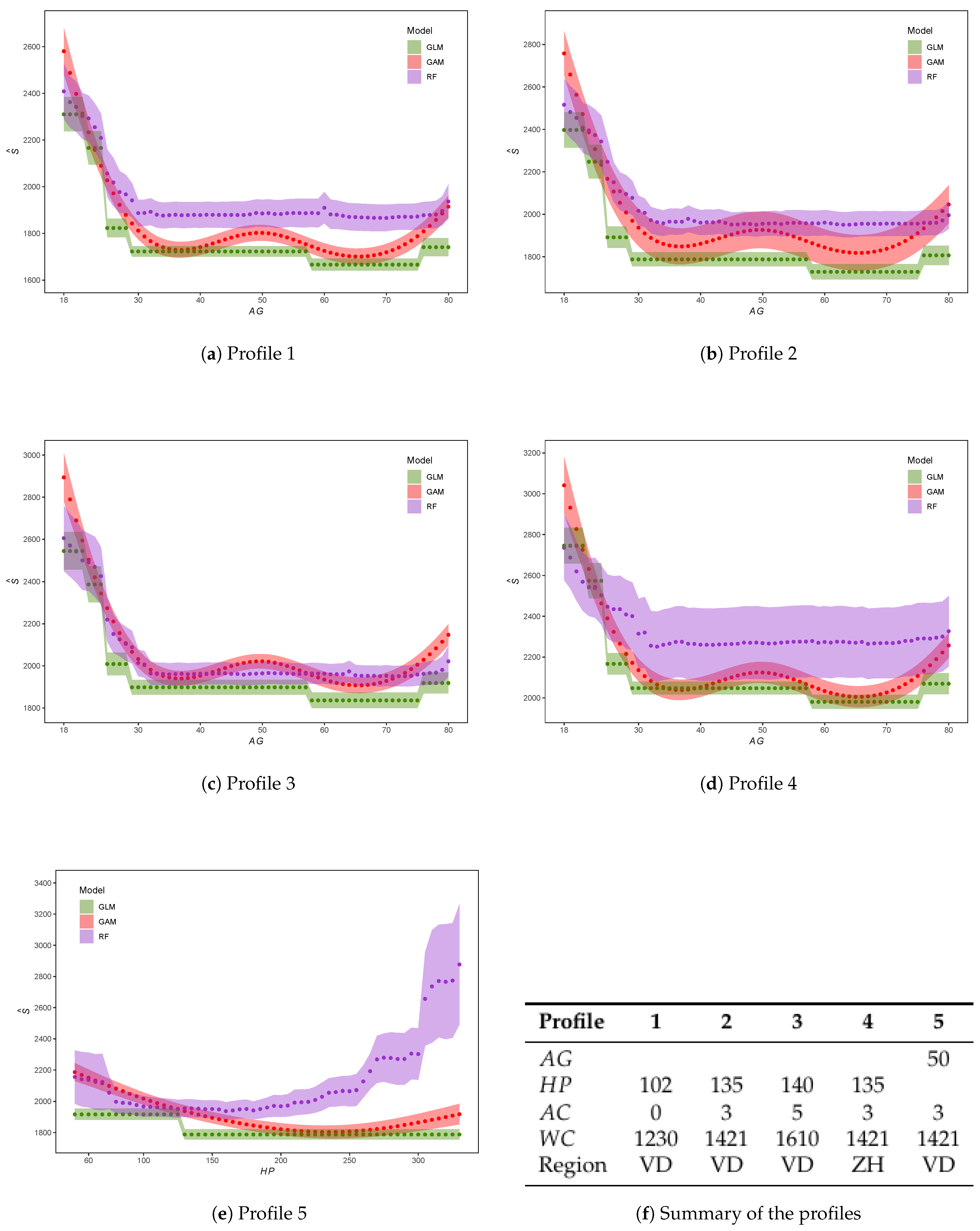
In the following, we compare the prediction performance of the models on the continuous variables age of the policyholder A G and horsepower of the car H P by fixing the other explanatory variables. Given the above performance statistics and because predictions are for log S , we do not consider the RF log S model in the sequel. Nevertheless, one of our objectives is to understand why the RF S model shows a lower performance on our data. In the following, we simplify the notation and write R F for RF S . For this analysis, we perform predictions for four profiles along the age A G (see Figure 12a–d) and for one profile along the horsepower H P (see Figure 12e). For the profiles, we consider a baseline contract of a male policyholder having Swiss nationality, a bonus-malus level protection with a bonus-malus level of 30%, and using the car privately with regular commuter routes. We consider a customer driving a three-year-old limousine with a value of CHF 33 900, no accessories and a policy deductible of CHF 300. The other variables age of the policyholder A G , horsepower H P , age A C , and weight W C of the car and the residence regions are varied along the values outlined in exhibit (f) of Figure 12. For profiles 1 to 4, the variations along ages are illustrated in graphs (a) to (d), while, for profile 5, the effect of horsepower is given in the graph (e). For all predictions, we provide 95%-confidence intervals: since these are point predictions, the confidence intervals are created with the help of the bootstrap ensemble technique, i.e., the variance of the predictions is obtained by creating 100 random training samples with replacements (Carney et al. 2003; Veaux et al. 2014).
Expectedly, we observe that the results from GAM exhibit smooth variations stemming from the smoothing splines used. The optimized bins that are created by the evolutionary trees and used in GLM are well visible along the age and horsepower variables (cf. Figure 2a,b). The predictions of the GAM and GLM conform with each other. RF presents partially significantly different predictions. For example, for ages below 30 years, the predicted claim severity S ^ from RF is decreasing with the age of the policyholder (see Figure 12a–d) comparably to GAM and GLM, but stays almost constant for ages from 30 to 80 years. The confidence intervals of the RF model often overlap the ones of the GAM and GLM, especially for younger ages from 18 to 30 years. While an overall agreement through the models exists along the age, we only find, in profile 1, that the RF confidence intervals do not overlap at higher ages. The predictions along the horsepower that are reported in Figure 11e are in agreement from 50 to 150. However, afterwards, RF results in higher predictions and the confidence intervals of the different models are distinct. The results of RF present many places where contiguous values of the risk factor lead to very different predictions. These findings may explain part of why the RF model yields high ABC and ICC values. In particular, we have observed that the results from the RF model do not vary along the ages from 30 to 80, which is leading to the RF model not covering the claims and the expected true premium of the portfolio.
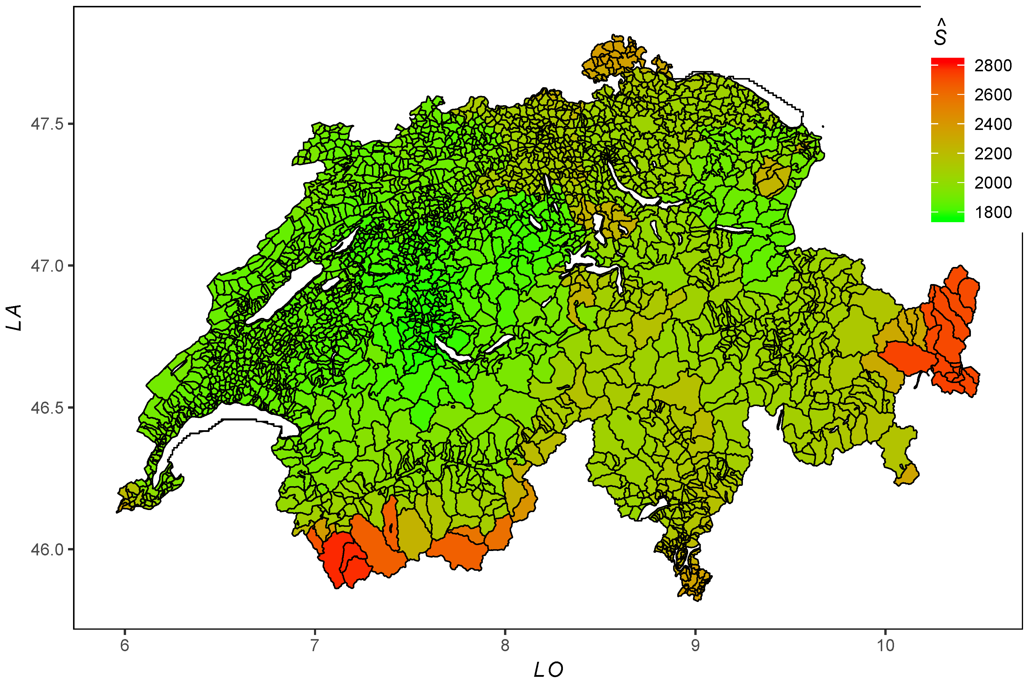
For the same baseline profile underlying Figure 12, we illustrate the spatial claim severity predictions for GAM, respectively RF S in Figure 13 and Figure 14. Thereby, we fix the age of the policyholder to 50 years, the horsepower of the car to 135, and the age and weight of the car to 3 years and 1 421 kg, respectively. We observe that the predictions that are illustrated in Figure 13 agree with the effects shown in Figure 3. As observed earlier while fitting the model, GAM predicts the highest claim severity for the Italian-speaking region and the lowest one for policyholders from the areas of Bern and St. Gallen. When considering Figure 14, we find that RF is not completely in line with the GAM results. In fact, certain policyholders from the Valais and Graubünden have a very high claim severity; higher variations are observed in the RF results. RF models seem to “react” much more importantly when there are differences between regions. Overall, we observe that the GAM is differentiating better along the longitude and latitude when compared to the RF model. This is in accordance with the results that were obtained in the figures above.

5. Conclusions

This paper compares the claim severity modeling and the predictions of GAM, GLM, and RF models when applied on the same car collision dataset from a Swiss insurer. In our application, based on a training sample, we build a forward and backward stepwise optimal GAM under the BIC for the severity S and derive from this model an optimized GLM with the help of evolutionary trees following the work of Henckaerts et al. (2018). The traditional regression models rely on a log-normal distribution implying an exponential back-transformation of the predictions. We also build two RF models using S and log ( S ) with the root mean squared error (RMSE) as an optimization function. We compare the performance of GAM, GLM, and RF models on a test sample by taking several perspectives considering individual and total errors, violin plots, and comparing the model predictions along selected profiles.
We observe that the log-normal assumption for the claim severity implies a non-trivial back-transformation of the predictions when aiming to measure the model performance (Ai and Norton 2000; Duan 1983). We use the GOF and GOL measures to evaluate the performance of the models (Denuit et al. 2019). The GOF and GOL are not simultaneously improved in a given model, so that they provide valuable insights together with the violin plots and the selected profile representations. No model is outperforming the other ones throughout all the criteria, in accordance with the results of Denuit et al. (2019) and Henckaerts et al. (2020). Nevertheless, the GAM seems to be the one with the best overall performance (and no extremely bad results in any dimension) on both training and test samples. The GLM built along Henckaerts et al. (2018) is also a valid model. However, this model leads to bad predictions on unseen data. GAM and RF have a much better performance on the test sample. The RF log S model does not cover the overall expenses, but it has a good coverage for the right-skewed part of the data. The weakness of the RF log S model are the large claims. Instead, the RF S model is well covering the overall expenses, but it iis not covering the premium needs for the claims and the true premium along the portfolio. For the application on profiles, we observe that the RF S model leads to the results with the lowest variations, whereas the GAM and GLM show much more variations along the age, the horse power, and the location. The final choice of the model will depend on the particular preferences and requirements on the model, e.g., for usage in claims predictions or ratemaking.
Further, based on our data covering the whole Switzerland, to the best of our knowledge, we are the first to provide evidence for the importance of detailed spatial information along longitude and latitude in Switzerland. The traditional cantonal segmentation can be largely improved by integrating local aspects that are related to urbanicity (urban and rural regions) and specific characteristics of the terrain (cities, mountains). Indeed, Figure 4 highlights relevant differences in the claim severity that are not linked to the boundaries of the Swiss cantons. For practitioners and actuaries, this finding can serve to have a better understanding to define relevant risk factors and categories and to choose a model. A more fine-grained classification of customers for their expected severity levels along regions helps to make models more precise and, e.g., to offer more adequate premiums, thus making a company’s ratemaking more competitive, as shown in the papers of Denuit and Lang (2004) and Klein et al. (2014).
Finally, when considering the observations that were made in the present case study, several open research questions remain. While, in this paper, we focus on the log-normal distribution assumption for our data and analyze the available back-transformation, additional insights could be generated by choosing other distributions for the claims, like, for example, a Gamma or inverse Gaussian distribution (see e.g., Henckaerts et al. 2020; Staudt et al. 2001), and to compare these results with the prediction performance obtained here. The back-transformation is leading to high discrepancies on the severity, which are not observed on the log scale. These differences could be analyzed with more details (see also Henckaerts 2020). The deviance measure could be applied to evaluate the model and be compared to the ones that were used here. A thorough analysis of the impact of the tuning parameters on the prediction performance and on the size of the confidence intervals should be performed. Partitioning-out analysis (Belloni et al. 2014; Chernozhukov et al. 2015) could be used to analyze the impact of the different variables in combination with the representations of the selected profiles. While our research compares two families of model, further research could investigate other models, as, for example, penalized regressions and evolutionary trees.

Author Contributions

Conceptualization, Y.S. and J.W.; methodology, Y.S. and J.W.; formal analysis, Y.S.; writing–original draft preparation, Y.S.; writing–review and editing, Y.S. and J.W.; supervision, J.W.; funding acquisition, J.W. Both authors have read and agreed to the published version of the manuscript.

Funding

Part of this research was carried out while Y.S. was employed by the University of Lausanne. This research received no additional external funding.

Data Availability Statement

Restrictions apply to the availability of these data. Data was obtained from a third party for the purpose of this study and the authors are not allowed to share the data.

Acknowledgments

Both authors thank the insurance company for providing the data for this research.

Conflicts of Interest

The authors declare no conflict of interest.

Appendix A

The following figures and tables provide additional information on the data and the regressions.
Figure A1. Illustration of the relative frequencies of the claim severity S along risk factors in the training sample.
Risks 09 00053 g0a1aRisks 09 00053 g0a1bRisks 09 00053 g0a1c
Table A1. Regression results of the GAM (Equation (1)) and GLM (Equation (3)) calibrated on the training sample.
GAM (1)GLM (3)
Intercept 7.161 *** 6.761 ***
B S (baseline: Yes)
    No 0.072 *** 0.072 ***
CS (baseline: CL)
    CH 0.024 * 0.024 *
    CC 0.121 *** 0.126 ***
    CO 0.195 *** 0.198 ***
CB g (baseline: VW)
    BMW 0.105 *** 0.116 ***
    Daimler 0.106 *** 0.099 ***
    Fiat 0.062 ** 0.067 **
    Ford 0.007 0.007
    GM 0.096 * 0.113 *
    Greely 0.007 0.004
    Honda 0.024 0.019
    Hyundai 0.035 0.026
    Independent 0.082 0.086
    Mazda 0.051 * 0.054 *
    PSA 0.132 *** 0.134 ***
    Renault 0.149 *** 0.155 ***
    Subaru 0.038 0.037
    Suzuki 0.207 *** 0.212 ***
    Tata 0.088 . 0.102 *
    Toyota 0.019 0.028
ID (baseline: 300)
    500 0.053 *** 0.052 ***
    1000 0.218 *** 0.221 ***
    ≥2000 0.487 *** 0.525 ***
f ^ 1 ( AG ) 7.009 *** AG c (baseline: 29–57)
    18 21 0.293 ***
    22 24 0.229 ***
    25 28 0.057 **
    58 75 0.033 **
    76 81 0.011
    > 81 0.196 ***
f ^ 2 ( HP ) 3.927 *** HP c (baseline: >126)
    41 125 0.070 ***
f ^ 3 ( AC ) 5.230 *** AC c (baseline: 0–3)
    4 0.069 ***
    5 0.097 ***
    6 0.158 ***
    7 0.178 ***
    > 8 0.269 ***
f ^ 4 ( WC ) 1.002 *** WC 0.0002 ***
f ^ 5 ( LO , LA ) 24.740 *** ( LO , LA ) c (baseline: 3)
    1 0.132 ***
    2 0.080 ***
    4 0.068 ***
    5 0.128 ***
    6 0.254 ***
    7 0.477 ***
BIC201,748 201,516
N65,950 65,950
Significance levels for p-values: *** p ≤ 0.001, ** p ≤ 0.01, * p ≤ 0.05, p ≤ 0.1.

References

  1. Ai, Chunrong, and Edward C. Norton. 2000. Standard errors for the retransformation problem with heteroscedasticity. Journal of Health Economics 19: 697–718. [Google Scholar] [CrossRef]
  2. Albrecher, Hansjoerg, Jan Beirlant, and Jef L. Teugels. 2017. Reinsurance: Actuarial and Statistical Aspects. Wiley Series in Probability and Statistics; Chichester: Wiley. [Google Scholar]
  3. Antonio, Katrien, and Emiliano A Valdez. 2012. Statistical Concepts of a Priori and a Posteriori Risk Classification in Insurance. Asta-Advances in Statistical Analysis 96: 187–224. [Google Scholar] [CrossRef] [Green Version]
  4. Bellina, Rémi. 2014. Méthodes D’apprentissage Appliquées à la Tarification Non-Vie. Lyon: Université Claude Bernard. [Google Scholar]
  5. Belloni, Alexandre, Victor Chernozhukov, and Lie Wang. 2014. Pivotal Estimation via Square-Root Lasso in Nonparametric Regression. Annals of Statistics 42: 757–88. [Google Scholar] [CrossRef]
  6. Bieck, Christian, Boderas Mareike, Peter Maas, and Tobias Schlager. 2010. Powerful Interaction Points: Saying Goodbye to the Channel. Somers: IBM Institute for Business Value and University of St. Gallen. [Google Scholar]
  7. Brisard, Evelien. 2014. Pricing of Car Insurance with Generalized Linear Models. Master’s thesis, Univeristé Libre de Bruxelles, Brussels, Belgium. [Google Scholar]
  8. Carney, John G., Padraig Cunningham, and Umesh Bhagwan. 2003. Confidence and prediction intervals for neural network ensembles. Paper presented at IJCNN’99, International Joint Conference on Neural Networks, Washington, DC, USA, July 10–16; Volume 2, pp. 1215–1218. [Google Scholar] [CrossRef]
  9. Chai, Tianfeng, and Roland R. Draxler. 2014. Root mean square error (RMSE) or mean absolute error (MAE)? -Arguments against avoiding RMSE in the literature. Geoscientific Model Development 7: 1247–50. [Google Scholar] [CrossRef] [Green Version]
  10. Charpentier, Arthur. 2014. Computational Actuarial Science with R. Boca Raton: CRC Press. [Google Scholar]
  11. Chernozhukov, Victor, Christian Hansen, and Martin Spindler. 2015. Valid Post-Selection and Post-Regularization Inference: An Elementary, General Approach. Annual Review of Economics 7: 649–88. [Google Scholar] [CrossRef] [Green Version]
  12. Cort, J. Willmott, and Matsuura Kenji. 2005. Advantages of the mean absolute error (MAE) over the root mean square error (RMSE) in assessing average model performance. Climate Research 30: 79–82. [Google Scholar] [CrossRef]
  13. Csorgo, Sandor, and Julian J. Faraway. 1996. The Exact and Asymptotic Distributions of Cramer-von Mises Statistics. Journal of the Royal Statistical Society Series B (Methodological) 58: 221–34. [Google Scholar] [CrossRef]
  14. Dalkilic, Turkan Erbay, Fatih Tank, and Kamile Sanli Kula. 2009. Neural networks approach for determining total claim amounts in insurance. Insurance: Mathematics and Economics 45: 236–41. [Google Scholar] [CrossRef]
  15. Denuit, Michel, Donatien Hainaut, and Julien Trufin. 2019a. Effective Statistical Learning Methods for Actuaries I: GLM and Extensions. Springer Actuarial. Cham: Springer International Publishing. [Google Scholar] [CrossRef]
  16. Denuit, Michel, Donatien Hainaut, and Julien Trufin. 2019b. Effective Statistical Learning Methods for Actuaries III. Springer Actuarial. Cham: Springer International Publishing. [Google Scholar] [CrossRef]
  17. Denuit, Michel, Donatien Hainaut, and Julien Trufin. 2020. Effective Statistical Learning Methods for Actuaries II. Springer Actuarial. Cham: Springer International Publishing. [Google Scholar] [CrossRef]
  18. Denuit, Michel, and Stefan Lang. 2004. Non-life Rate-making with Bayesian GAMs. Insurance: Mathematics and Economics 35: 627–47. [Google Scholar] [CrossRef]
  19. Denuit, Michel, Xavier Marechal, Sandra Pitrebois, and Jean-Francois Walhin. 2007. Actuarial Modelling of Claim Counts: Risk Classification, Credibility and Bonus-Malus Systems. Hoboken: John Wiley & Sons, Inc. [Google Scholar]
  20. Denuit, Michel, Dominik Sznajder, and Julien Trufin. 2019. Model selection based on Lorenz and concentration curves, Gini indices and convex order. Insurance: Mathematics and Economics 89: 128–39. [Google Scholar] [CrossRef] [Green Version]
  21. Dewi, Kartika Chandra, Hendri Murfi, and Sarini Abdullah. 2019. Analysis Accuracy of Random Forest Model for Big Data—A Case Study of Claim Severity Prediction in Car Insurance. Paper presented at 2019 5th International Conference on Science in Information Technology: Embracing Industry 4.0: Towards Innovation in Cyber Physical System, ICSITech 2019, Jogja, Indonesia, October 23–24; pp. 60–65. [Google Scholar] [CrossRef]
  22. Dougherty, James, Ron Kohavi, and Mehran Sahami. 1995. Supervised and Unsupervised Discretization of Continuous Features. Machine Learning: Proceedings of the Twelfth International Conference 12: 194–202. [Google Scholar] [CrossRef] [Green Version]
  23. Duan, Naihua. 1983. Smearing Estimate: A Nonparametric Retransformation Method. Journal of the American Statistical Association 78: 605. [Google Scholar] [CrossRef]
  24. Durbin, James. 1973. Distribution Theory for Tests Based on the Sample Distribution Function. Philadelphia: Society for Industrial and Applied Mathematics. [Google Scholar]
  25. Eling, Martin. 2014. Fitting Asset Returns to Skewed Distributions: Are the Skew-Normal and Skew-Student Good Models? Insurance: Mathematics and Economics 59: 45–56. [Google Scholar] [CrossRef]
  26. Ferrario, Andrea, Alexander Noll, and Mario V. Wüthrich. 2018. Insights from Inside Neural Networks. SSRN Electronic Journal. [Google Scholar] [CrossRef]
  27. Frees, Edward W., Gee Lee, and Lu Yang. 2016. Multivariate Frequency-Severity Regression Models in Insurance. Risks 4: 4. [Google Scholar] [CrossRef] [Green Version]
  28. Frees, Edward W. 2015. Analytics of Insurance Markets. Annual Review of Financial Economics 7: 253–77. [Google Scholar] [CrossRef] [Green Version]
  29. Frees, Edward W., Richard A. Derrig, and Glenn Meyers. 2016. Predictive Modeling Applications in Actuarial Science Volume 1: Predictive Modeling Techniques. Cambridge: Cambridge University Press. [Google Scholar] [CrossRef]
  30. Grubinger, Thomas, Achim Zeileis, and Karl-Peter Pfeiffer. 2014. Evtree: Evolutionary Learning of Globally Optimal Classification and Regression Trees in R. Journal of Statistical Software 61: 1. [Google Scholar] [CrossRef] [Green Version]
  31. Guelman, Leo. 2012. Gradient boosting trees for auto insurance loss cost modeling and prediction. Expert Systems with Applications 39: 3659–67. [Google Scholar] [CrossRef]
  32. Guelman, Leo, Montserrat Guillén, and Ana M. Pérez-Marín. 2012. Random Forests for Uplift Modeling: An Insurance Customer Retention Case BT—Modeling and Simulation in Engineering, Economics and Management. Berlin/Heidelberg: Springer, pp. 123–33. [Google Scholar]
  33. Hastie, Trevor, Robert Tibshirani, and Jerome Friedman. 2009. The Elements of Statistical Learning: Data Mining, Inference, and Prediction, 2nd ed. New York: Springer. [Google Scholar]
  34. Hastie, Trevor J., and Robert J. Tibshirani. 1990. Generalized Additive Models. Boca Raton: CRC Press. [Google Scholar]
  35. Henckaerts, Roel. 2020. DistRforest: Distribution-Based Random Forest. github. Available online: https://github.com/henckr/distRforest (accessed on 20 February 2021).
  36. Henckaerts, Roel, Katrien Antonio, Maxime Clijsters, and Roel Verbelen. 2018. A Data Driven Binning Strategy for the Construction of Insurance Tariff Classes. Scandinavian Actuarial Journal 1238: 1–25. [Google Scholar] [CrossRef] [Green Version]
  37. Henckaerts, Roel, Marie Pier Côté, Katrien Antonio, and Roel Verbelen. 2020. Boosting Insights in Insurance Tariff Plans with Tree-Based Machine Learning Methods. North American Actuarial Journal, 1–31. [Google Scholar] [CrossRef]
  38. Hu, Sen, Adrian O’Hagan, James Sweeney, and Mohammadhossein Ghahramani. 2020. A spatial machine learning model for analysing customers’ lapse behaviour in life insurance. Annals of Actuarial Science 2020: 1–27. [Google Scholar] [CrossRef]
  39. Huang, Yifan, and Shengwang Meng. 2019. Automobile insurance classification ratemaking based on telematics driving data. Decision Support Systems 127: 113156. [Google Scholar] [CrossRef]
  40. James, Gareth, Daniela Witten, Trevor Hastie, and Robert Tibshirani. 2013. An Introduction to Statistical Learning with Applications in R. New York: Springer. [Google Scholar] [CrossRef]
  41. Kamakura, Wagner A., Michel Wedel, Fernando de Rosa, and Jose Afonso Mazzon. 2003. Cross-Selling through Database Marketing: A mixed Data Factor Analyzer for Data Augmentation and Prediction. International Journal of Research in Marketing 20: 45–65. [Google Scholar] [CrossRef] [Green Version]
  42. Abbas, Khosravi, Saeid Nahavandi, Doug Creighton, and Amir F. Atiya. 2011. Comprehensive Review of Neural Network-Based Prediction Intervals and New Advances. IEEE Transactions on Neural Networks 22: 1341–56. [Google Scholar] [CrossRef]
  43. Klein, Nadja, Michel Denuit, Stefan Lang, and Thomas Kneib. 2014. Nonlife Ratemaking and Risk Management with Bayesian Generalized Additive Models for Location, Scale, and Shape. Insurance: Mathematics and Economics 55: 225–49. [Google Scholar] [CrossRef]
  44. Kuhn, Max. 2008. Building Predictive Models in R Using the caret Package. Journal of Statistical Software 28: 5. [Google Scholar] [CrossRef] [Green Version]
  45. Kuhn, Max, and Kjell Johnson. 2013. Applied Predictive Modeling. New York: Springer. [Google Scholar] [CrossRef]
  46. Laas, Daniela, Hato Schmeiser, and Joël Wagner. 2016. Empirical Findings on Motor Insurance Pricing in Germany, Austria and Switzerland. The Geneva Papers on Risk and Insurance-Issues and Practice 41: 398–431. [Google Scholar] [CrossRef]
  47. Li, Yaqi, Chun Yan, Wei Liu, and Maozhen Li. 2018. A principle component analysis-based random forest with the potential nearest neighbor method for automobile insurance fraud identification. Applied Soft Computing Journal 70: 1000–9. [Google Scholar] [CrossRef]
  48. Longford, Nicholas T. 2009. Inference with the lognormal distribution. Journal of Statistical Planning and Inference 139: 2329–40. [Google Scholar] [CrossRef] [Green Version]
  49. Lowe, Julian, and Louise Pryor. 1996. Neural Networks v. GLMs in pricing general insurance. Working Paper presented at Insurance Convention. [Google Scholar]
  50. Lüdi, Georges, and Iwar Werlen. 2005. Sprachenlandschaft in der Schweiz. Neuchâtel: Swiss Federal Statistical Office. [Google Scholar]
  51. Maas, Peter, Albert Graf, and Christian Bieck. 2008. Trust, Transparency and Technology. Somers: IBM Institute for Business Value and University of St. Gallen. [Google Scholar]
  52. Manning, Willard G. 1998. The logged dependent variable, heteroscedasticity, and the retransformation problem. Journal of Health Economics 17: 283–95. [Google Scholar] [CrossRef]
  53. Manning, Willard G., and John Mullahy. 2001. Estimating log models: To transform or not to transform? Journal of Health Economics 20: 461–94. [Google Scholar] [CrossRef] [Green Version]
  54. Nelder, John Ashworth, and Robert WM Wedderburn. 1972. Generalized Linear Models. Journal of the Royal Statistical Society. Series A (General) 135: 370–84. [Google Scholar] [CrossRef]
  55. Nicholls, Anthony. 2014. Confidence limits, error bars and method comparison in molecular modeling. Part 1: The calculation of confidence intervals. Journal of Computer-Aided Molecular Design 28: 887–918. [Google Scholar] [CrossRef] [PubMed] [Green Version]
  56. Noll, Alexander, Robert Salzmann, and Mario V. Wüthrich. 2018. Case Study: French Motor Third-Party Liability Claims. SSRN Electronic Journal. [Google Scholar] [CrossRef]
  57. Ohlsson, Esbjörn, and Björn Johansson. 2010. Non-Life Insurance Pricing with Generalized Linear Models. EAA SERIES. Berlin/Heidelberg: Springer. [Google Scholar] [CrossRef]
  58. Pelessoni, Renato, and Liviana Picech. 1998. Some applications of unsupervised neural networks in rate making procedure. Paper presented at Insurance Convention and ASTIN Colloquium, Glasgow, Scotland, October 7–10. [Google Scholar]
  59. Perla, Francesca, Ronald Richman, Salvatore Scognamiglio, and Mario V. Wuthrich. 2020. Time-Series Forecasting of Mortality Rates using Deep Learning. SSRN Electronic Journal. [Google Scholar] [CrossRef]
  60. Quan, Zhiyu, and Emiliano A. Valdez. 2018. Predictive analytics of insurance claims using multivariate decision trees. Dependence Modeling 6: 377–407. [Google Scholar] [CrossRef]
  61. Richman, Ronald. 2018. AI in Actuarial Science. SSRN Electronic Journal. [Google Scholar] [CrossRef]
  62. Schelldorfer, Jürg, and Mario V. Wüthrich. 2019. Nesting Classical Actuarial Models into Neural Networks. SSRN Electronic Journal. [Google Scholar] [CrossRef]
  63. Schwarz, Gideon. 1978. Estimating the Dimension of a Model. The Annals of Statistics 6: 461–64. [Google Scholar] [CrossRef]
  64. Slocum, Terry A., Robert B. McMaster, Fritz C. Kessler, and Hugh H. Howard. 2005. Thematic Cartography and Geographic Visualization. Upper Saddle River: Pearson Prentice Hall. [Google Scholar]
  65. Staudt, Yves, Julien Trufin, and Joël Wagner. 2001. Goodness of Lift in Collision Insurance. Working Paper. Lausanne: University of Lausanne. [Google Scholar]
  66. Staudt, Yves, and Joël Wagner. 2018. What Policyholder and Contract Features Determine the Evolution of Non-life Insurance Customer Relationships?: A Case Study Analysis. International Journal of Bank Marketing 36: 1098–124. [Google Scholar] [CrossRef] [Green Version]
  67. Staudt, Yves, and Joël Wagner. 2019. Comparison of Machine Learning and Traditional Severity-Frequency Regression Models for Car Insurance Pricing. Working Paper. Lausanne: University of Lausanne. [Google Scholar]
  68. Staudt, Yves, and Joël Wagner. 2020. Duration to Cross-selling in Non-life Insurance: New Empirical Evidence from Switzerland. Working Paper. Lausanne: University of Lausanne. [Google Scholar]
  69. De Vleaux, Richard D., Jennifer Schumi, Jason Schweinsberg, and Lyle H. Ungar. 2014. Intervals Prediction for Neural Networks via Nonlinear Regression. Technometrics 40: 273–82. [Google Scholar] [CrossRef]
  70. Velthoen, Jasper, Clément Dombry, Juan-Juan Cai, and Sebastian Engelke. 2021. Gradient Boosting for Extreme Quantile Regression. Working Paper. Delft: Delft University of Technology. [Google Scholar]
  71. Verbelen, Roel, and Katrien Antonio. 2016. Unraveling the Predictive Power of Telematics Data in Car Insurance Pricing. SSRN Electronic Journal. [Google Scholar] [CrossRef] [Green Version]
  72. Wang, Yibo, and Wei Xu. 2018. Leveraging deep learning with LDA-based text analytics to detect automobile insurance fraud. Decision Support Systems 105: 87–95. [Google Scholar] [CrossRef]
  73. Willmott, Cort J., Kenji Matsuura, and Scott M. Robeson. 2009. Ambiguities inherent in sums-of-squares-based error statistics. Atmospheric Environment 43: 749–52. [Google Scholar] [CrossRef]
  74. Wüthrich, Mario V., and Christoph Buser. 2018. Data Analytics For Non-Life Insurance Pricing. SSRN Electronic Journal. [Google Scholar] [CrossRef]
1.
In fact, a very small share of claims is not closed and our data report mostly identical reserves for each open claim making such records hard to interpret. By omitting open claims, which may relate to more difficult cases and higher amounts, we keep in mind that the overall claim distribution might differ and that our findings underestimate the total claim amount. Nevertheless, the basis for the study is the same for all of the considered models, allowing for us to compare them.
2.
These results reach the boundary of our tuning grid and an ad hoc analysis beyond this point was conducted. The analysis does not bring new insights that would differ from the one obtained at the boundary. Thus, we keep the graphics with the same α -axis, which allows for simple comparisons among the cases.
Figure 1. Illustration of the distribution of the claim severity S in the training dataset.
Risks 09 00053 g001
Figure 2. Illustration of the generalized additive models (GAM) effects ( f ^ 1 , f ^ 2 , f ^ 3 and f ^ 4 ) in Equation (1) and the bins obtained from evolutionary trees for the age of the policyholder A G , the horsepower H P , the age A C and the weight W C of the car.
Risks 09 00053 g002
Figure 3. Illustration of the spatial GAM effect f 5 ^ ( L O , L A ) along longitude and latitude.
Risks 09 00053 g003
Figure 4. Illustration of the BIC as a function of the penalization parameter α for the evolutionary trees in the case of A G , H P and A C and as a function of the number of bins n for Fisher’s natural breaks in the case of ( L O , L A ) .
Risks 09 00053 g004
Figure 5. Illustration of the optimal classification of the spatial information along Fisher’s natural breaks.
Risks 09 00053 g005
Figure 6. Illustration of the R M S E ¯ model error and 95%-confidence intervals for different values of the number of risk factors m and the minimum node size for both RF log S and RF S models.
Risks 09 00053 g006
Figure 7. Illustration of the R M S E ¯ model error and 95%-confidence intervals along the number of trees B for both RF log S and RF S models.
Risks 09 00053 g007
Figure 8. Illustration of the residuals and the predictions for the models using log S .
Risks 09 00053 g008
Figure 9. Illustration of the A B C and I C C GOL statistics in the training and test samples.
Risks 09 00053 g009
Figure 10. Comparison of the violin plots across the GAM, GLM and RF models in the training and test samples.
Risks 09 00053 g010
Figure 11. Illustration of the A B C and I C C GOL statistics for log S in the training and test samples.
Risks 09 00053 g011
Figure 12. Comparison of the predicted claim severity S ^ with 95%-confidence intervals along different ages (in graphs a to d for profiles 1 to 4) and horsepower values (in graph e for profile 5) across the GAM, GLM, and RF models.
Risks 09 00053 g012
Figure 13. Illustration of the spatial claim severity predictions for the GAM in Equation (1).
Risks 09 00053 g013
Figure 14. Illustration of the spatial claim severity predictions for the RF S model.
Risks 09 00053 g014
Table 1. Summary of the variables that are available in the data.
VariableDescription
Continuous variables
    A G Age of the policyholder (in years)
    B M Bonus-malus level (in %)
    H P Horsepower of the vehicle (in hp)
    V C Value of the car without accessories (in CHF)
    A P Value of the accessories of the car as a percentage of the car value
    A C Age of the car (in years)
    W C Weight of the car (in kg)
    L O Longitude of the policyholder’s main residence ( 6.0 10.5 E)
    L A Latitude of the policyholder’s main residence ( 45.8 47.8 N)
Categorical variables
    CA 26 cantons of Switzerland and Principality of Liechtenstein
    LR Language regions along three classes: German, French, Italian
    NA Nationality along the following classes: Switzerland (CH), France (FR), Germany and Austria (DE-AT), Spain (ES), Portugal (PT), Italy (IT), Eastern Europe and Turkey (EE-TR), other (OT)
    UT Utilization along three classes: private use with/without irregular commuter route (PE), private use with regular commuter route (PR), professional use (PL)
    CS Car body style along four classes: hatchback and sedan (CH), limousine (CL), convertible (CC), other (CO)
    CB Car brand
    CB g Car brand group
    CB c Car brand country
    NS Number of seats along three classes: 4 , 5 and 6 + seats
    ID Deductible along four classes: CHF 300, 500, 1000 and 2000 +
Binary variables
    G E Gender of the policyholder (male/female)
    I T Online contract underwriting (yes/no)
    B S Bonus-malus level protection (yes/no)
    P M Zero-alcohol engagement (yes/no)
    D W Driving license withdrawal (yes/no)
    D D Driving less than 10 , 000  km per year (yes/no)
Table 2. GOF statistics for the distribution of the claim severity S in the training dataset.
DistributionWeibullGammaLog-Normal
KS0.0570.0680.043
CvM96.328110.97334.269
BIC1,150,2001,150,4691,147,293
Table 3. Comparison of the total predicted severity i S ^ i , goodness-of-fit statistics (GOF) and goodness-of-lift statistics (GOL) across the generalized additive models (GAM), generalized linear models (GLM), and random forests (RF) models in the training sample.
DataGAMGLM RF log S RF S
Training sample (data from 2011–2014)
    i S ^ i (in CHF)149.3 mio149.5 mio148.4 mio87.2 mio149.0 mio
    RE 0.29 % 0.37 % 41.4 % 0.04%
    RMSE 3047304930532860
    MAE 1730173214161650
    ABC ( · 10 3 ) 4.45.1112.996.7
    ICC 0.4560.4560.3240.364
Table 4. Comparison of the total predicted claim severity i S ^ i , GOF and GOL across the GAM, GLM, and RF models in the test sample.
DataGAMGLM RF log S RF S
Test sample (data from 2015)
    i S ^ i (in CHF)34.9 mio34.8 mio34.9 mio20.3 mio34.8 mio
    RE 0.24%0.08%41.9%0.16%
    RMSE 2964296531142957
    MAE 1689169215211701
    ABC ( · 10 3 ) 5.6437.2525.3969.915
    ICC 0.4580.4590.4580.454
Table 5. Comparison of the total predicted claim severity GOF and GOL across the GAM, GLM, and RF models in the training and samples for log S .
GAMGLM RF log S
Training sample (data from 2011–2014)
    RMSE1.1111.1111.113
    MAE0.8370.8370.839
    ABC ( · 10 3 )0.2500.1072.150
    ICC0.4970.4980.498
Test sample (data from 2015)
    RMSE1.0631.0641.062
    MAE0.8050.8050.803
    ABC ( · 10 3 )0.2550.4140.2314
    ICC0.4980.4980.498
Publisher’s Note: MDPI stays neutral with regard to jurisdictional claims in published maps and institutional affiliations.