Quantifying the Role of Occurrence Losses in Catastrophe Excess of Loss Reinsurance Pricing

Abstract

The aim of this paper is to merge order statistics with natural catastrophe reinsurance pricing to develop new theoretical and practical insights relevant to market practice and model development. We present a novel framework to quantify the role that occurrence losses (order statistics) play in pricing of catastrophe excess of loss (catXL) contracts. Our framework enables one to analytically quantify the contribution of a given occurrence loss to the mean and covariance structure, before and after the application of a catXL contract. We demonstrate the utility of our framework with an application to idealized catastrophe models for a multi-peril and a hurricane-only case. For the multi-peril case, we show precisely how contributions to so-called lower layers are dominated by high frequency perils, whereas higher layers are dominated by low-frequency high severity perils. Our framework enables market practitioners and model developers to assess and understand the impact of altered model assumptions on the role of occurrence losses in catXL pricing.

1. Introduction

Reinsurance companies sell products that allow primary insurers to improve their portfolio return profiles through risk transfer. Suppose a primary insurer exclusively underwrites homeowner policies in the state of California. Due to a lack of ability to diversify geographically (say across the United States), over the course of any particular annual insurance cycle, the primary insurer may build up a portfolio with poor risk adjusted returns, and could lack access to cost efficient capital to cover all potential liabilities. A variety of reinsurance products can be purchased by primary insurers to improve risk/return profiles and protect against extreme losses. One of the most important products is the so-called catastrophe excess of loss (catXL) contract (Cummins et al. 1999; Hurlimann 2005; Mata 2000). CatXL contracts allow insurers to protect against extreme losses arising from perils such as hurricane, windstorms, convective storms, earthquakes, flooding, wildfires and storm surge. CatXL contracts are also used in transferring other types of risk such as life risk (Ekheden and Hossjer 2014). Reinsurers sell a variety of catXL contracts with the aim of building a diversified portfolio with attractive returns on capital over the long run. Risk transfer through catXL contract underwriting plays a fundamental and important role in the global reinsurance marketplace (Cummins et al. 1999).

Reinsurers use various metrics to decide whether or not any particular catXL contract should be underwritten. The metrics include loss results obtained from catastrophe simulation models used in technical pricing (defined in the main body), market dynamics that determine the supply and demand for reinsurance, brokerage fees, metrics which quantify the diversification benefit of any incremental addition of risk to a portfolio, risk appetite and capital availability. Underwriting decisions and portfolio construction are functions of these factors. This paper focuses on catastrophe simulation model output in relation to technical pricing.

In the vast majority of cases, catastrophe models are built using complex physical simulations of natural hazard phenomena (Michel 2018; Mitchell-Wallace et al. 2017). Physically based simulations of hazard are fed into so-called vulnerability models which assess the damage arising from any particular event occurrence to a portfolio of physical risks (Michel 2018; Mitchell-Wallace et al. 2017). The next step is for the physical damage to be converted into financial loss reported at various levels of aggregation (e.g., location and portfolio level). In this paper, we conceptualize catastrophe model output by working with a so-called timeline simulation of event losses, obtained by running the model against a portfolio of physical risks. We assume that for a given portfolio of risks, the timeline simulation can be obtained by simulating from a frequency distribution and a portfolio specific severity distribution (analogous to actuarial applications (Klugman et al. 2008)). We assume that both frequency and severity are independent (commonly assumed in actuarial applications (Klugman et al. 2008), although recent studies explore the relaxation of this assumption (Peng et al. 2015)). In some instances, the frequency and severity distributions may have exact analytical forms, but this need not be the case. Most catXL contracts apply to a one-year period (Cummins et al. 1999; Hurlimann 2005; Mata 2000) which is the focus of this paper. Each year of simulation contains what are commonly referred to as occurrence losses in the catastrophe modeling community (Michel 2018; Mitchell-Wallace et al. 2017), consisting of the first, second, third and so on annual maximum losses. In statistics, the occurrence losses are commonly referred to as the order statistics (David and Nagaraja 2003). We use occurrence losses and order statistics synonymously in this paper. This paper addresses the role of occurrence losses in pricing catXL contracts.

The case of interest in this paper is the theory of order statistics with random sample sizes (drawn from specific frequency distributions), for which the theoretical underpinnings were established in a series of papers dating back to the 1970s (Barakat and El-Shandidy 2015; Buhrman 1973; Consul 1984; Gupta and Gupta 1984; Raghunandanan and Patil 1976; Young 1970). Analytical methods for pricing catXL contracts have been extensively studied in the literature (Cummins et al. 1999; Hurlimann 2005; Mata 2000). The aim of this paper is to merge order statistics and catXL reinsurance pricing to address a number of practical and theoretical questions related to the role of occurrence losses in catXL pricing. The types of questions motivating this work are as follows:

• What is the contribution of the second largest annual hurricane loss to a given catXL technical price, and how does the contribution depend on catastrophe model assumptions?
• How do the contributions from various occurrence losses vary as a function of the catXL contract specification? Furthermore, how does this inform which perils are most important for different risk takers in the market?
• How well converged are the occurrence loss contributions (in a finite simulation) before and after the application of a catXL contract?
• What is the correlation structure of occurrence losses, before and after applying a catXL contract, and what role does the correlation play in quantifying pricing metrics?

In this paper, we develop a novel mathematical framework that enables one to analytically decompose various technical catXL pricing metrics into contributions from the occurrence losses. We are not aware of any similar studies in the literature. We demonstrate the utility of our framework numerically using two idealized catastrophe models for US nationwide multi-peril losses and hurricane-only losses. In particular for the multi-peril case: We demonstrate, in a precise way, how so-called lower layers (oftentimes retained by primary insurers) are dominated by high-frequency perils, whereas higher layers (typically covered by reinsurers) are dominated by low-frequency high severity perils. Such insights are useful for both market practitioners and catastrophe model developers alike.

This paper is organized as follows. In Section 2, we present analytical results for occurrence losses and catXL pricing. We show the general expression for the distribution of occurrence losses (for discrete frequency and continuous severity), and show the application of this to the Poisson and Negative Binomial frequency cases (both of which are frequently used in applications). We demonstrate how mean losses, both before (pre) and after (post) the application of a catXL contract, can be decomposed into the sum of integrals on the individual occurrence loss distributions. We also provide expressions which can be used to quantify the covariance structure of the occurrence losses for the pre and post catXL perspectives. Finally, we show how to quantify convergence errors (arising from finite simulation sets used in practical settings) associated with various occurrence loss metrics (mean, standard deviation, correlation) pre and post catXL. In Section 3, we apply our mathematical framework to a representative US nationwide portfolio comprised of hurricane, wildfire, severe convective storm, winter storm and earthquake risks, enabling us to address the questions raised in this paper. In Section 4, we provide a sensitivity study for a US hurricane-only model to address questions related to model adequacy that arise in practice. Section 5 provides a summary, draws conclusions, and discusses new avenues of suggested research.

2. A Mathematical Framework for Occurrence Losses in Reinsurance Pricing

We begin this section with a mathematical formulation of a catastrophe model characterized by a frequency and severity distribution. The catastrophe model is used to generate what we refer to as a ‘timeline simulation’, which is the typical starting point for pricing reinsurance contracts. We assume the timeline simulation has periods of one-year in length. We provide the mathematical definition of occurrence loss random variables (corresponding to the ordered maxima in each one-year period). Two cases are of interest: Before (pre) and after (post) the application of a catXL reinsurance contract. We define $Z_{pre}$ as a random variable corresponding to the annual sum of occurrence losses before the application of a catXL. $Z_{post}$ is defined as the annual sum of occurrence losses after the application of a catXL. Market practitioners use functions of the mean and variance of $Z_{post}$ as inputs to a catXL pricing formula. Motivated by market practice, and to address the types of questions which are central to this paper, we demonstrate how to $decompose$ the mean and variance of $Z_{post}$ into $contributions$ from the various occurrence losses. We also do the same for the mean and variance of $Z_{pre}$ to gain additional insights. The required mathematical results are provided in what follows. We end this section by addressing how to quantify convergence errors that arise in practical applications.

2.1. Preliminaries

We first provide all the necessary mathematical definitions and notation that are used throughout this work.

2.1.1. Frequency

Let N be a discrete random variable representing the annual number of events for a catastrophe model. N is drawn from $P_N(N=k)$ where $k\in [0,1,2,3,\dots ]$, and ${\sum }_{k=0}^{\infty }{P}_N(N=k)=1$. We make use of two particular frequency distributions due to their common application in catastrophe modeling (Michel 2018; Mitchell-Wallace et al. 2017).

The first is the Negative Binomial distribution given by,

$$P_{nb,N}(N=k)=\frac{\Gamma (k+r)}{k!\Gamma \left(r\right)}{p}^r{(1-p)}^k$$

(1)

where $r=\frac{{\mu }^2}{{\sigma }^2-\mu }>0$, $\Gamma \left(r\right)$ is the gamma function $\Gamma \left(r\right)={\int }_0^{\infty }{s}^{r-1}{e}^{-s}ds$ (for $r>0$) (Bahnemann 2015), $p=\frac{\mu }{{\sigma }^2}$, with mean $E_N\left[N\right]=\mu$ and variance $Va{r}_N\left[N\right]={\sigma }^2$ (Klugman et al. 2008). Subscript $nb$ is used to indicate Negative Binomial. The Negative Binomial distribution is ‘over-dispersive’ with $\frac{{\sigma }^2}{\mu }>1$.

A special case of the Negative Binomial is given by the limit as $r\to \infty$, yielding the Poisson distribution,

$$P_{pois,N}(N=k)=\frac{e^{-\lambda }{\lambda }^k}{k!}$$

(2)

with expectation $E_N\left[N\right]=\lambda$ and variance $Va{r}_N\left[N\right]=\lambda$ (Klugman et al. 2008). Subscript $pois$ makes clear the Poisson case. The over-dispersion, defined as the ratio of the variance to the mean, is 1.

2.1.2. Severity

In this paper, we discuss losses to a portfolio of physical asset risks insured by a primary insurer. Given an event occurrence, the primary insurer portfolio level financial loss (in $) due to the event is assumed to be drawn from a continuous severity distribution with density $f_X\left(x\right)$ and cumulative probability $F_X\left(x\right)$.

2.1.3. Independence Assumptions for Single and Multi-Peril Models

We assume that samples from the frequency $P_N(N=k)$ and severity $f_X\left(x\right)$ are generated independently. Typically, in practical applications, $P_N(N=k)$ and $f_X\left(x\right)$ is used to represent one particular peril (e.g., US hurricane) against one specific primary insurer portfolio.

We can also represent multiple perils (causing losses on the same portfolio) as follows. Let P represent the number of perils. For each of the $p=1,2,\dots ,P$ perils, the severity distribution is given by $f_{X_p}\left(x\right)$. We assume that the severity distribution for all perils combined is given by the mixture $f_X\left(x\right)={\sum }_{p=1}^P{w}_p{f}_{X_p}\left(x\right)$, where ${\sum }_{p=1}^P{w}_p=1$. Each of the perils has its own frequency distribution $P_{N_p}(N_p=k_p)$, and we assume the multi-peril frequency random variable is given by $N={\sum }_{p=1}^P{N}_p$. Frequency and severity are also assumed to be independent in the multiple-peril case.

2.1.4. Notation

In this paper, we adopt classical compound claims notation with a slight deviation from convention to meet the needs of this paper. Given the frequency N, the event losses drawn from the (single or multi-peril) severity $f_X\left(x\right)$ are denoted by: $X_1,X_2,\dots ,X_N$. Here we use the convention that $X_1\ge X_2\ge \dots \ge X_N$. Therefore $X_1$ represents the annual maximum, $X_2$ represents the second annual maximum, and so on. These ordered random variables are called the occurrence losses.

For our purposes, it is convenient to extend this classical notation in the following sense. First, suppose that the random frequency $N=k$. In this case, the particular event losses are denoted by: $(X_1=x_1)\ge (X_2=x_2)\ge \dots \ge (X_k=x_k)\ge (X_{k+1}=0)\dots \ge (X_{\infty }=0)$. We use the convention that all event losses with index greater than k are assigned a value of zero (this is of course true as they do not occur). This notation convention is useful as we are interested in the statistics of all occurrence losses.

Given the above discussion, we hereafter denote the occurrence loss random variables as $X_M$ where $M\in [1,2,3,\dots ]$ (where $X_1\ge X_2$ and so on). Next we discuss how the statistics of the occurrence loss random variables can be used to understand reinsurance pricing.

2.1.5. Pre-catXL Loss Perspective and Decomposition

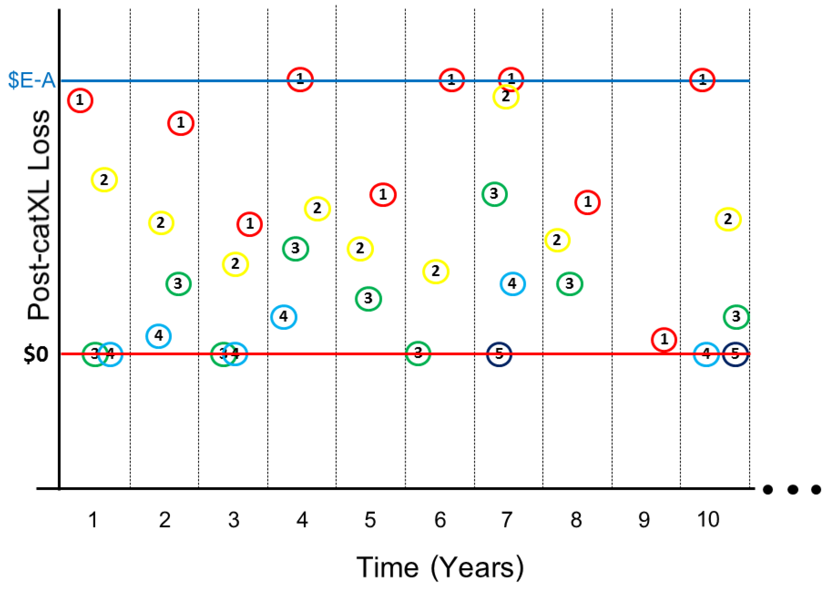
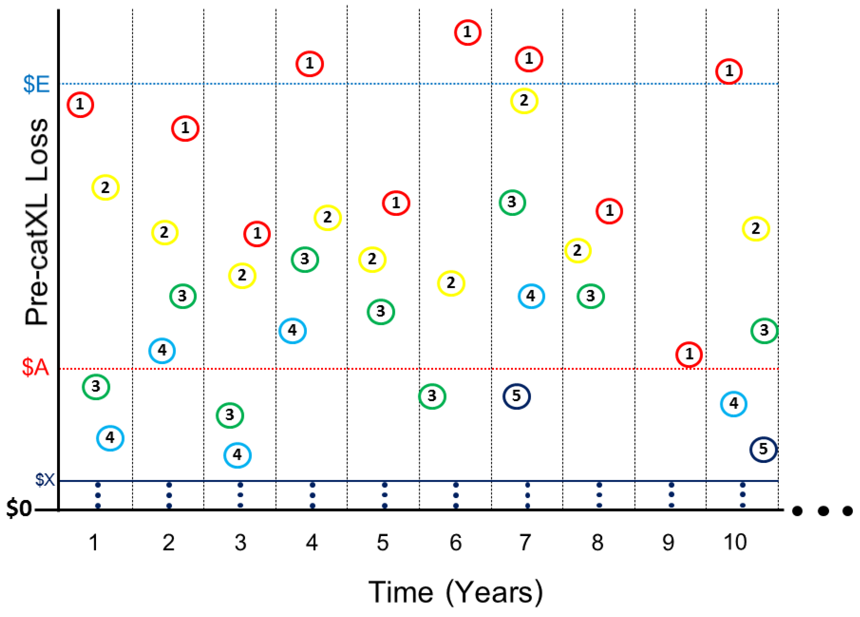
We now discuss what we call the pre-catXL perspective, which considers losses to a primary insurer portfolio $before$ the application of any reinsurance. For any given model described by frequency $P_N(N=k)$ and severity $f_X\left(x\right)$, we can generate what we call a ‘timeline simulation’ by using the following procedure: 1. For each year $i=1,\dots ,S$ of simulation, generate a random draw from $P_N(N=k)$ denoted by $k_i$. 2. Then take $k_i$ independent samples from the severity $f_X\left(x\right)$. A visualization of a timeline simulation is provided in Figure 1. For example, in year $i=1$ we have 4 losses above the loss threshold $\$X$. The dots below the loss threshold $\$X$ represent the 5th largest loss and so on. Suppose for year $i=7$ the realization of N is $k_7=5$, then the 6th smallest loss and beyond is assigned 0.

In each year of simulation, there is a 1st maximum, a 2nd maximum, and so on, as labeled in Figure 1. These ordered maxima are what we call the occurrence losses. Figure 1 shows that events happen at different times of year (as in reality). To simplify, we ignore this ‘seasonality’. Using the above stated notation, the random variable $X_M$, where $M\in [1,2,3,\dots ]$, is called the Mth annual maximum loss. We also define the annual aggregate loss $Z_{pre}={\sum }_{M=1}^{\infty }{X}_M$ (subscript $pre$ emphasizes pre-catXL perspective).

Our aim is to quantify the contribution of the various occurrence losses to the mean and variance of $Z_{pre}$. This is motivated by the fact that the mean and variance are inputs to technical pricing metrics used in making reinsurance underwriting decisions (discussed in what follows). It is therefore of interest to understand the mean and variance before the application of reinsurance, to enable better understanding of what are the effects of applying reinsurance structures. We emphasize the fact that the variance depends on the correlation structure and is therefore of interest.

Mathematically, we require the mean ${\mu }_{X_M}$ and variance ${\sigma }_{X_M}^2$ for all M. We also require an expression for the Pearson correlation between any arbitrary pair of occurrence loss random variables indexed by $I,J\in [1,2,3,\dots ]$, where $I>J$, written as ${\rho }_{X_I,X_J}$. Analytical expressions for all these quantities provided in Section 2.3, Section 2.4 and Section 2.5 (with derivations in Appendices Appendix A, Appendix B and Appendix C).

We now define the decomposition of the mean and variance of $Z_{pre}$, which is our main tool for analysis in this paper. The mean of $Z_{pre}$ is given by,

$$E_X\left[Z_{pre}\right]\equiv AA{L}_{pre}=\sum _{M=1}^{\infty }{\mu }_{X_M}$$

where $AA{L}_{pre}$ denotes the pre-catXL average annual aggregate loss. The contribution $C_{AA{L}_{pre},X_M}$ of any particular occurrence loss $X_M$ to the $AA{L}_{pre}$ is defined as,

$$C_{AA{L}_{pre},X_M}=\frac{{\mu }_{X_M}}{AA{L}_{pre}}$$

(3)

where ${\sum }_{M=1}^{\infty }{C}_{AA{L}_{pre},M}=1$ ($AA{L}_{pre}$ is assumed finite).

For the annual aggregate loss variance, $Va{r}_{pre}$, we take the variance over all occurrence loss random variables $X_M$. Using the expression for the variance of the sum of correlated random variables, we obtain,

$$Va{r}_{pre}=\sum _{M=1}^{\infty }{\sigma }_{X_M}^2+\sum _{1\le J<I<\infty }2{\rho }_{X_I,X_J}{\sigma }_{X_I}{\sigma }_{X_J}$$

and we define the marginal contribution $C_{Va{r}_{pre},X_M}$ of any particular occurrence loss $X_M$ to $Va{r}_{pre}$ as,

$$C_{Va{r}_{pre},X_M}=\frac{{\sigma }_{X_M}^2}{Va{r}_{pre}}$$

(4)

and we define the interaction contribution $C_{Va{r}_{pre},X_I,X_J}$ of any pair of occurrence losses $X_I$ and $X_J$ to be $Va{r}_{pre}$ as,

$$C_{Va{r}_{pre},X_I,X_J}=\frac{2{\rho }_{X_I,X_J}{\sigma }_{X_I}{\sigma }_{X_J}}{Va{r}_{pre}}$$

(5)

where ${\sum }_{M=1}^{\infty }{C}_{Va{r}_{pre},X_M}+{\sum }_{1\le J<I<\infty }{C}_{Va{r}_{pre},X_I,X_J}=1$ ($Va{r}_{pre}$ is assumed finite).

2.1.6. Post-catXL Loss Perspective and Decomposition

We now apply the reinsurance layer depicted in Figure 1 by the so-called attachment point $\$A$ and exhaustion point $\$E$. Figure 2 gives a visual representation of the effect of applying the layer parameterized by $\$A$ and $\$E$. Mathematically, this is represented by the following random variable,

$$Y_{AE,M}=\left\{\begin{array}{c}\begin{array}{cc}0& X_M<A\\ X_M-A& A\le X_M<E\\ E-A& X_M\ge E\end{array}\end{array}\right.$$

where $M\in [1,2,3,\dots ]$ (and $Y_{AE,1}\ge Y_{AE,2}$ and so on). This can be written in a compact form as $Y_{AE,M}=Min[Max[0,X_M-A],E-A]$ (Cummins et al. 1999; Hurlimann 2005; Mata 2000). In this paper, we develop analytical expressions for the mean ${\mu }_{Y_{AE,M}}=E_X\left[Y_{AE,M}\right]$, the variance ${\sigma }_{Y_{AE,M}}^2=Va{r}_X\left[Y_{AE,M}\right]$, and the correlation coefficient ${\rho }_{Y_{AE,I},Y_{AE,J}}$ between any pair of random variables $Y_{AE,I}$ and $Y_{AE,J}$ with $I,J\in [1,2,3,\dots ]$ and $I>J$. Analytical expressions for all these quantities are shown in Section 2.3, Section 2.4 and Section 2.5 (with derivations in Appendices Appendix A, Appendix B and Appendix C). Subscript $AE$ specifies a particular $\$A$ and $\$E$.

The reinsurer is responsible for all the losses depicted in Figure 2 up to a certain limit called the (annual) aggregate limit $\$AL=(1+re)(\$E-\$A)$, where $re\in [0,1,2,\dots ]$ specifies the number of ‘reinstatements’ (as in Cummins et al. 1999; Hurlimann 2005; Mata 2000). Typical market practice is to set the number of reinstatements $re$ to 2 or 3. For simplicity, we make the assumption that $re\to \infty$. Previous studies have found that pricing metrics based on 2 or 3 reinstatements are well approximated by results using the limit $re\to \infty$ (Khare et al. 2015). Assuming $re\to \infty$, the annual aggregate loss random variable is given by the sum over all occurrence losses so that $Z_{post,AE}={\sum }_{M=1}^{\infty }{Y}_{AE,M}$ (where subscript post denotes after application of the catXL layer). A given combination of $\$A$ and $\$E$ is called a ‘layer’.

Common market practice makes use of the mean and variance of $Z_{post,AE}$ to compute what we call technical prices which are used to make underwriting decisions. For example, a technical pricing metric could be computed as,

$$\frac{E_X\left[Z_{post,AE}\right]+v\sqrt{Va{r}_X\left[Z_{post,AE}\right]}}{premium}$$

where $premium$ denotes net income, and v is a volatility loading factor greater than 0. Decomposing the mean $E_X\left[Z_{post,AE}\right]$ and variance $Va{r}_X\left[Z_{post,AE}\right]$ into the contributions from the various underlying occurrence losses will enable us to understand the role that they play in the technical pricing. We emphasize again that the total variance $Va{r}_X\left[Z_{post,AE}\right]$ depends on the correlation ${\rho }_{Y_{AE,I},Y_{AE,J}}$, motivating our analysis of the correlation structure to follow.

We now define the decomposition of the mean and variance of $Z_{post,AE}$, which is our main tool for analysis in this paper. In the uncapped aggregate limit where $re\to \infty$, the post-catXL mean annual aggregate loss is simply obtained by summing the post-catXL mean annual losses for each random variable $Y_{AE,M}$ given by,

$$E_X\left[Z_{post,AE}\right]\equiv AA{L}_{post,AE}=\sum _{M=1}^{\infty }{\mu }_{Y_{AE,M}}.$$

The contribution $C_{AA{L}_{post},Y_{AE,M}}$ of any particular occurrence loss $Y_{AE,M}$ to the $AA{L}_{post,AE}$ is defined by,

$$C_{AA{L}_{post},Y_{AE,M}}=\frac{{\mu }_{Y_{AE,M}}}{AA{L}_{post,AE}}$$

(6)

where ${\sum }_{M=1}^{\infty }{C}_{AA{L}_{post},Y_{AE,M}}=1$ ($AA{L}_{post,AE}$ is assumed finite).

The annual aggregate loss variance, $Va{r}_{post,AE}$, is obtained using the formula for the variance of the sum of correlated random variables given by,

$$Va{r}_{post,AE}=\sum _{M=1}^{\infty }{\sigma }_{Y_{AE,M}}^2+\sum _{1\le J<I<\infty }2{\rho }_{Y_{AE,I},Y_{AE,J}}{\sigma }_{Y_{AE,I}}{\sigma }_{Y_{AE,J}}$$

and we define the marginal contribution $C_{Va{r}_{post},Y_{AE,M}}$ of any particular occurrence loss $Y_{AE,M}$ to be $Va{r}_{post,AE}$ as,

$$C_{Va{r}_{post},Y_{AE,M}}=\frac{{\sigma }_{Y_{AE,M}}^2}{Va{r}_{post,AE}}$$

(7)

and we define the interaction contribution $C_{Va{r}_{pre},Y_{AE,I},Y_{AE,J}}$ of any pair of occurrence losses $Y_{AE,I}$ and $Y_{AE,J}$ to be $Va{r}_{post,AE}$ as,

$$C_{Va{r}_{post},Y_{AE,I},Y_{AE,J}}=\frac{2{\rho }_{Y_{AE,I},Y_{AE,J}}{\sigma }_{Y_{AE,I}}{\sigma }_{Y_{AE,J}}}{Va{r}_{post,AE}}$$

(8)

where ${\sum }_{M=1}^{\infty }{C}_{Va{r}_{post},Y_{AE,M}}+{\sum }_{1\le J<I<\infty }{C}_{Va{r}_{post},Y_{AE,I},Y_{AE,J}}=1$ ($Va{r}_{post,AE}$ is assumed finite).

2.2. Occurrence Loss Marginal Distributions

Here we start with the general expression for the cumulative probability of any occurrence loss random variable $X_M$, written as an infinite sum. We then show expressions for the Negative Binomial (Equation (1)) and the limiting Poisson case (Equation (2)). Derivations are provided in the Appendix A.

2.2.1. General Expression

For convenience, we define the cumulative probability of the severity at loss threshold l as $f\equiv F_X\left(l\right)={\int }_0^l{f}_X\left(x\right)dx$. The cumulative probability $f\in [0,1]$ is not to be confused with the density $f_X\left(x\right)$. For any occurrence loss random variable $X_M$, the cumulative probability at l is given by,

$$F_{X_M}\left(l\right)=\sum _{k=0}^{M-1}{P}_N(N=k)+\sum _{k=M}^{\infty }{P}_N(N=k)\sum _{i=0}^{M-1}\left(\genfrac{}{}{0pt}{}{k}{k-i}\right)f^{k-i}{(1-f)}^i.$$

(9)

2.2.2. Negative Binomial Frequency Assumption

For any occurrence loss random variable $X_M$, and under the assumption that the frequency distribution is Negative Binomial (Equation (1)), the cumulative probability at loss threshold l is given by,

$$\begin{array}{c}\hfill F_{nb,X_M}\left(l\right)=\sum _{k=0}^{M-1}\frac{\Gamma (k+r)}{k!\Gamma \left(r\right)}{p}^r{(1-p)}^k-\sum _{i=0}^{M-1}\sum _{k=i}^{M-1}\frac{\Gamma (k+r)}{k!\Gamma \left(r\right)}{p}^r{(1-p)}^k\left(\genfrac{}{}{0pt}{}{k}{k-i}\right)f^{k-i}{(1-f)}^i\\ \hfill +\frac{p^r}{\Gamma \left(r\right)}\sum _{i=0}^{M-1}\frac{\Gamma (i+r){(1-f)}^i{(1-p)}^i{(1-f(1-p))}^{-(i+r)}}{i!}.\end{array}$$

(10)

2.2.3. Poisson Frequency Assumption

In the limit that $r\to \infty$ we obtain the Poisson frequency with corresponding marginal distribution,

$$F_{pois,X_M}\left(l\right)=\sum _{k=0}^{M-1}\frac{e^{\lambda }{\lambda }^k}{k!}-\sum _{i=0}^{M-1}\sum _{k=i}^{M-1}\frac{e^{\lambda }{\lambda }^k}{k!}\left(\genfrac{}{}{0pt}{}{k}{k-i}\right)f^{k-i}{(1-f)}^i+e^{-\lambda (1-f)}\sum _{i=0}^{M-1}\frac{{(1-f)}^i{\lambda }^i}{i!}.$$

(11)

2.3. Occurrence Mean Loss

We now build up the tools required to compute the decompositions for the pre and post-catXL annual aggregate loss means given by Equations (3) and (6). We start with the pre-catXL mean loss for any random variable $X_M$, given by,

$${\mu }_{X_M}={\int }_0^{\infty }(1-F_{freq,X_M}\left(x\right))dx$$

(12)

and for the post-catXL case, the mean loss associated with random variable $Y_{AE,M}$ is given by,

$${\mu }_{Y_{AE,M}}={\int }_A^E(1-F_{freq,X_M}\left(x\right))dx.$$

(13)

For completeness, derivations of Equations (12) and (13) are provided in the Appendix B.

2.4. Occurrence Loss Variance

To compute the marginal contributions to the total variance for $Z_{pre}$ and $Z_{post}$ (Equations (4) and (7)), we require the pre-catXL centered variance given by,

$${\sigma }_{X_M}^2={\int }_0^{\infty }2x(1-F_{freq,X_M}\left(x\right))dx-{\mu }_{X_M}^2$$

(14)

and for the post-catXL variance given by,

$${\sigma }_{Y_{AE,M}}^2={\int }_A^{E}2(x-A)(1-F_{freq,X_M}\left(x\right))dx-{\mu }_{Y_{AE,M}}^2.$$

(15)

Derivations of Equations (14) and (15) are provided in Appendix B.

2.5. Occurrence Loss Correlation Structure

To compute the interaction contributions to the total variance for $Z_{pre}$ and $Z_{post}$ (Equations (5) and (8)), we require expressions for the correlation coefficients between occurrence loss random variables. For convenience, we first define the operator $t_{AE}\left(\right)$ to be such that $t_{AE}\left(X_M\right)=Y_{AE,M}$. For any pair of random variables $Y_{AE,I}$ and $Y_{AE,J}$ ($I>J$ with $(I,J)\in [1,2,3,\dots ]$), the correlation coefficient, for a Negative Binomial frequency assumption, is given by the following double integral,

$$\begin{array}{c}\hfill {\rho }_{nb,Y_{AE,I},Y_{AE,J}}=\frac{1}{{\sigma }_{Y_{AE,I}}{\sigma }_{Y_{AE,J}}}({\mu }_{Y_{AE,I}}{\mu }_{Y_{AE,I}}\sum _{k=0}^{J-1}\frac{\Gamma (k+r)}{k!\Gamma \left(r\right)}{p}^r{(1-p)}^k\\ \hfill -{\mu }_{Y_{AE,I}}{\int }_0^{\infty }\left[(t_{AE}\left(y\right)-{\mu }_{Y_{AE,J}})\sum _{k=J}^{I-1}\frac{\Gamma (k+r)p^r{(1-p)}^k}{\Gamma \left(r\right)(k-J)!(J-1)!}{\left[F_X\left(y\right)\right]}^{k-J}{[1-F_X\left(y\right)]}^{J-1}{f}_X\left(y\right)\right]dy\\ \hfill +{\int }_{y=x}^{\infty }{\int }_0^{\infty }\left[(t_{AE}\left(x\right)-{\mu }_{Y_{AE,I}})(t_{AE}\left(y\right)-{\mu }_{Y_{AE,J}})A{3}_{nb}(x,y)\right]dxdy)\end{array}$$

(16)

where ${\sigma }_{Y_{AE,I}},{\sigma }_{Y_{AE,J}},{\mu }_{Y_{AE,I}},{\mu }_{Y_{AE,J}}$ are computed for Negative Binomial assumption. The pre-catXL case is covered by taking the limit as $A=0$ and $E\to \infty$ (so $t_{AE}\left(X_M\right)=X_M$). Equation (16) is derived in the Appendix C (where we also define $A{3}_{nb}(x,y)$). Equations (5), (8), (14)–(16) can be used to compute the pre and post-catXL interaction contributions (Negative Binomial case).

The Poisson case is obtained by taking the limit as $r\to \infty$ of Equation (16) and is given by,

$$\begin{array}{c}\hfill {\rho }_{pois,Y_{AE,I},Y_{AE,J}}=\frac{1}{{\sigma }_{Y_{AE,I}}{\sigma }_{Y_{AE,J}}}({\mu }_{Y_{AE,I}}{\mu }_{Y_{AE,J}}\sum _{k=0}^{J-1}\frac{e^{-\lambda }{\lambda }^k}{k!}\\ \hfill -{\mu }_{Y_{AE,I}}{\int }_0^{\infty }\left[(t_{AE}\left(y\right)-{\mu }_{Y_{AE,J}})\sum _{k=J}^{I-1}\frac{e^{-\lambda }{\lambda }^k}{(k-J)!(J-1)!}{\left[F_X\left(y\right)\right]}^{k-J}{[1-F_X\left(y\right)]}^{J-1}{f}_X\left(y\right)\right]dy\\ \hfill +{\int }_{y=x}^{\infty }{\int }_0^{\infty }\left[(t_{AE}\left(x\right)-{\mu }_{Y_{AE,I}})(t_{AE}\left(y\right)-{\mu }_{Y_{AE,J}})A{3}_{pois}(x,y)\right]dxdy)\end{array}$$

(17)

where ${\sigma }_{Y_{AE,I}},{\sigma }_{Y_{AE,J}},{\mu }_{Y_{AE,I}},{\mu }_{Y_{AE,J}}$ are computed for the Poisson assumption. Again, the pre-catXL result is obtained when $A=0$ and $E\to \infty$. Equation (17) is derived in the Appendix C (where we also define $A{3}_{pois}(x,y)$). Equations (5), (8), (14), (15) and (17) can be used to compute the pre and post-catXL interaction contributions (Poisson case).

2.6. Convergence Error Quantification

Typical market practice uses a limited number S years of simulation for technical reinsurance pricing. We are therefore interested in quantifying convergence errors associated with the various contributions to the mean and variance of $Z_{post}$ and $Z_{pre}$ arising from the occurrence losses of order M. Making use of the mathematical results provided above, we now discuss how this can be done using standard errors (Wasserman 2004). As there are a number of cases to cover, we first define some simplifying notation. Let $\mu$ and $\sigma$ be the mean and standard deviation for a given occurrence loss order M, frequency assumption, $\$A$ and $\$E$ ($\mu$ and $\sigma$ are not to be confused with the parameters discussed in Section 2.1.1). We also require the 4th central moment ${\mu }_4$ (the required integral is provided in the Appendix B). Let $\rho$ be the correlation coefficient between any pair of occurrence losses $Y_{AE,I}$ and $Y_{AE,J}$ (or $X_I$ and $X_J$ in the pre-catXL case). All values for $\mu$, $\sigma$, $\rho$ and ${\mu }_4$ are computed via numerical integration (to a high degree of accuracy for the numerical results discussed in Section 3 and Section 4).

2.6.1. Mean Loss

The standard error of the mean loss ($S{E}_{\mu }$) is given by,

$$S{E}_{\mu }=\frac{\sigma }{\sqrt{S}}$$

(18)

EECS (2021). Equation (18) quantifies the standard deviation of the mean loss over many independent simulation sets (Wasserman 2004). We define the percentage error to be $100\frac{\sigma }{\sqrt{S}\mu }$ where $\mu$ is the associated mean loss.

2.6.2. Variance

The standard error of the variance is given by,

$$S{E}_{{\sigma }^2}={\sigma }^2\sqrt{\frac{2}{S-1}}$$

(19)

EECS (2021). The percentage error is $100\sqrt{\frac{2}{S-1}}$ (which does not depend on a numerical estimate of ${\sigma }^2$).

2.6.3. Standard Deviation

The standard error of the standard deviation is approximately given by,

$$S{E}_{\sigma }\approx \frac{1}{2\sigma }\sqrt{\frac{1}{S}({\mu }_4-\frac{S-1}{S-3}{\sigma }^4)}$$

(20)

Rao (1973), and the percentage error is approximately $\frac{50}{{\sigma }^2}\sqrt{\frac{1}{S}({\mu }_4-\frac{S-1}{S-3}{\sigma }^4)}$.

2.6.4. Pearson Correlation

Here we consider a pair of occurrence loss random variable $Y_{AE,I}$ and $Y_{AE,J}$ where $I>J$ (the pair is $X_I$ and $X_J$ in the pre-catXL case). Suppose we generate many simulations of length S (starting with different random seeds) and for each simulation we use the sample statistics to estimate the correlation between $Y_{AE,I}$ and $Y_{AE,J}$. For each independent simulation of length S, let the random sample correlation coefficient be ${\rho }^{\ast }\left(S\right)$. If $Y_{AE,I}$ and $Y_{AE,J}$ are normally distributed, we know that the random variable $Z=\frac{1}{2}ln\left(\frac{1+{\rho }^{\ast }\left(S\right)}{1-{\rho }^{\ast }\left(S\right)}\right)$ is approximately normally distributed with mean equal to $E\left[Z\right]=\frac{1}{2}ln\left(\frac{1+\rho }{1-\rho }\right)$ (where $\rho$ is the true correlation), and variance $Var\left[Z\right]=\frac{1}{S-3}$ (Fisher 1915, 1921). It is clear that $Y_{AE,I}$ and $Y_{AE,J}$ are not generally bi-variate normal (Equations (9)–(11)). Despite this, we simply choose to apply the results for the bi-variate normal to derive an approximate confidence interval for $\rho$ as a function of S. We can form a confidence interval for Z as, $[E\left[Z\right]-\sqrt{\frac{1}{S-3}},E\left[Z\right]+\sqrt{\frac{1}{S-3}}]$. Given that ${\rho }^{\ast }\left(S\right)=\frac{e^{2Z}-1}{e^{2Z}+1}$, we can invert this expression to derive an approximate confidence interval for $\rho$,

$$\left[\frac{e^{2(E\left[Z\right]-\sqrt{\frac{1}{S-3}})}-1}{e^{2(E\left[Z\right]-\sqrt{\frac{1}{S-3}})}+1},\frac{e^{2(E\left[Z\right]+\sqrt{\frac{1}{S-3}})}-1}{e^{2(E\left[Z\right]+\sqrt{\frac{1}{S-3}})}+1}\right]$$

(21)

Let L be the length of the above confidence interval. We define the percentage error as $100\frac{L}{2\rho }$ (the factor of 2 divides the asymmetric interval length in half).

3. Multi-Peril Model Results for a US Nationwide Portfolio

We now apply our mathematical framework to an idealized representation of a multi-peril catastrophe model for a US nationwide industry portfolio. We begin by prescribing an appropriate frequency and severity, followed by an analysis of the resulting risk profile to set the context. We then analyze the decompositions of the AAL and total variance of the pre and post-catXL perspectives, which demonstrates the practical insights that are gained by application of our framework.

3.1. Multi-Peril Model Setup and Risk Profile

Our objective is to define a multi-peril frequency and severity model that will serve as a reasonable testbed for our mathematical framework from which we can derive practical insight. First we define the perils, their respective AALs and average annual frequencies, followed by our formulation of the severity distribution.

We use publicly available data from (AON 2021; Insurance Information Institute 2021) to formulate model parameters such that the model is representative of results from a catastrophe model run against a US nationwide insured portfolio. We assume that losses on a hypothetical US industry portfolio arise from hurricanes (HU), winter storms (WS), wildfires (WF), earthquakes (EQ) and severe convective storms (SCS). Using the US inflation-adjusted losses from 1980–2018 provided in (Insurance Information Institute 2021) as a guide, we assume a portfolio AAL of $29.5 Billion (hereafter denoted by B). We then use Exhibit 19 of (Insurance Information Institute 2021) as a guide to assign the following AALs to each peril: $12.5 B to HU, $2.5 B to WS, $2.5 B to WF, $2.0 B to EQ and $10.0 B to SCS. Historical frequency data of US loss events provided in (Insurance Information Institute 2021) (1980–2018) suggests that order 100 meteorological events occur on average where the vast majority of events are severe convective storms. We therefore assign an average annual frequency of 100 to SCS, and we assign to 2 to HU and 6 to WS (we use the ratio of HU to WS loss events provided in (Insurance Information Institute 2021)). Insurance Information Institute (2021) also provides frequency data for geological events, and we assign a frequency of 5 to EQ. Finally, we assign a frequency of 70 to WF. This deviates from the data provided in (Insurance Information Institute 2021), but our choice reflects the fact that many small WF events occur that may not be accounted in (Insurance Information Institute 2021) due to censoring, and also noting that the annual frequency of WF events is order 50,000 (CRS 2021). The perils, assigned AALs and average annual frequencies are provided in the first 3 Columns of

Table 1. This table contains the assumed parameters for the individual peril frequency and severity distributions that are used to form the multi-peril catastrophe model studied in this paper. Column 1 provides the peril names. Column 2 provides the average annual loss (AAL) for each peril against a hypothetical industry portfolio. Column 3 provides the average annual frequency of loss causing events per peril. Column 4 provides the coefficient of variation for each perils’ respective severity distribution. Columns 5 and 6 give the $\alpha$ and $\beta$ parameters of the gamma distribution used to model the severity distribution for each peril. The multi-peril model is formed using a mixture of the various peril frequency and severity distributions as described in the main text.

Peril	AAL ($ Billion)	Frequency	CV	$\mathit{\alpha }$	$\mathit{\beta }$
Hurricane (HU)	12.5	2	5	0.04	1.56 $\times {10}^{11}$
Winter Storm (WS)	2.5	6	3	0.11	3.75 $\times {10}^9$
Wildfire (WF)	2.5	70	8	0.016	2.19 $\times {10}^9$
Earthquake (EQ)	2.0	5	10	0.01	4.0 $\times {10}^{10}$
Convective Storm (SCS)	10.0	100	4	0.063	1.6 $\times {10}^9$

.

The severity distribution for each individual peril is assumed to be a gamma distribution. The gamma density is given by $f_X\left(x\right)=\frac{1}{\Gamma \left(\alpha \right){\beta }^{\alpha }}{x}^{\alpha -1}{e}^{-\frac{x}{\beta }}$ for $x>0$, and $f_X\left(x\right)=0$ for $x\in (-\infty ,0]$, where $\alpha >0$ is the shape parameter, $\beta >0$ is the scale parameter, and the gamma function $\Gamma \left(\alpha \right)$ (Section 2.1.1). The mean event loss is $\alpha \beta$ with variance $\alpha {\beta }^2$. We note that the gamma distribution is used in actuarial based reinsurance applications (Bahnemann 2015), and was therefore deemed sufficient for demonstration purposes only. Alternative severity distributions may result in different conclusions, but we leave exploration of this issue to future work. To determine the shape and scale parameters for each distribution, we note that the mean event loss $\alpha \beta$ is given by the AAL divided by the average annual frequency. We now impose an assumption on the coefficient of variation (CV) given by the event loss standard deviation divided by the event loss mean. For HU we simply $assume$ this to be equal to 5. Given a mean event loss of $6.25 B, this implies that a 1 standard deviation event gives a loss of order $30 B, and a 2 standard deviation event gives a loss of order $60 B, which is reasonable given historical losses (Insurance Information Institute 2021). Using the HU value of CV as a baseline, we then assign CV values for other perils using sensible relativities. We assume EQ has a CV exactly twice that of HU. We assume both WS and SCS are less volatile than HU with assigned values of 3 and 4 respectively, whereas WF is more volatile so we have assigned a CV value of 8. With these (reasonable) assumptions in hand, we can readily solve for the shape and scale parameters $\alpha ,\beta$, whose numerical values are provided in Columns 4 and 5 of Table 1.

Having chosen the individual peril parameters in Table 1, we can now formulate the multi-peril frequency and severity given certain assumptions. We assume that each peril has independent frequency and severity. We also assume independence across perils. We assume each individual peril has a Poisson frequency, which under our stated assumptions implies that the multi-peril frequency is also a Poisson distribution with average annual frequency $\lambda =183$ (Klugman et al. 2008). The multi-peril severity is taken to be a weighted mixture of the underlying gamma distributions for the different perils (with weights proportional to a given perils Frequency in Table 1 divided by the total multi-peril $\lambda =183$). The multi-peril frequency and severity are assumed independent (as stated in Section 2.1.3).

To set the context, we now analyze the implied risk profile of our multi-peril frequency and severity model. In Figure 3, we display results from a $S=$ 500,000 year timeline simulation (details of the simulation method are provided in Appendix D). The colored dots in the first 5 panels represent individual annual aggregate losses for WS, WF, SCS, HU and EQ. The horizontal axis (for each peril) is the log (base 10) of the annual aggregate loss in USD. The bars overlaid on top of the colored dots represent the minimum, maximum, median and interquartile ranges. The corresponding histograms are displayed on top of the individual colored dots. The final row labeled ALL displays results aggregated across all perils. Figure 3 demonstrates a number of qualitative features of our modeling setup. First, it is clear that both HU and EQ are the most volatile of the 5 perils with potential loss years greater than $100 Billion USD. Figure 3 makes clear that tail risk is dominated by HU followed by EQ. Both SCS and WF have a tighter range of annual aggregate losses which is consistent with the high frequency nature of both perils. The results for ALL perils combined demonstrates a large variation in aggregate annual losses from the tens of Billions USD to over one Trillion USD in the most of extreme years.

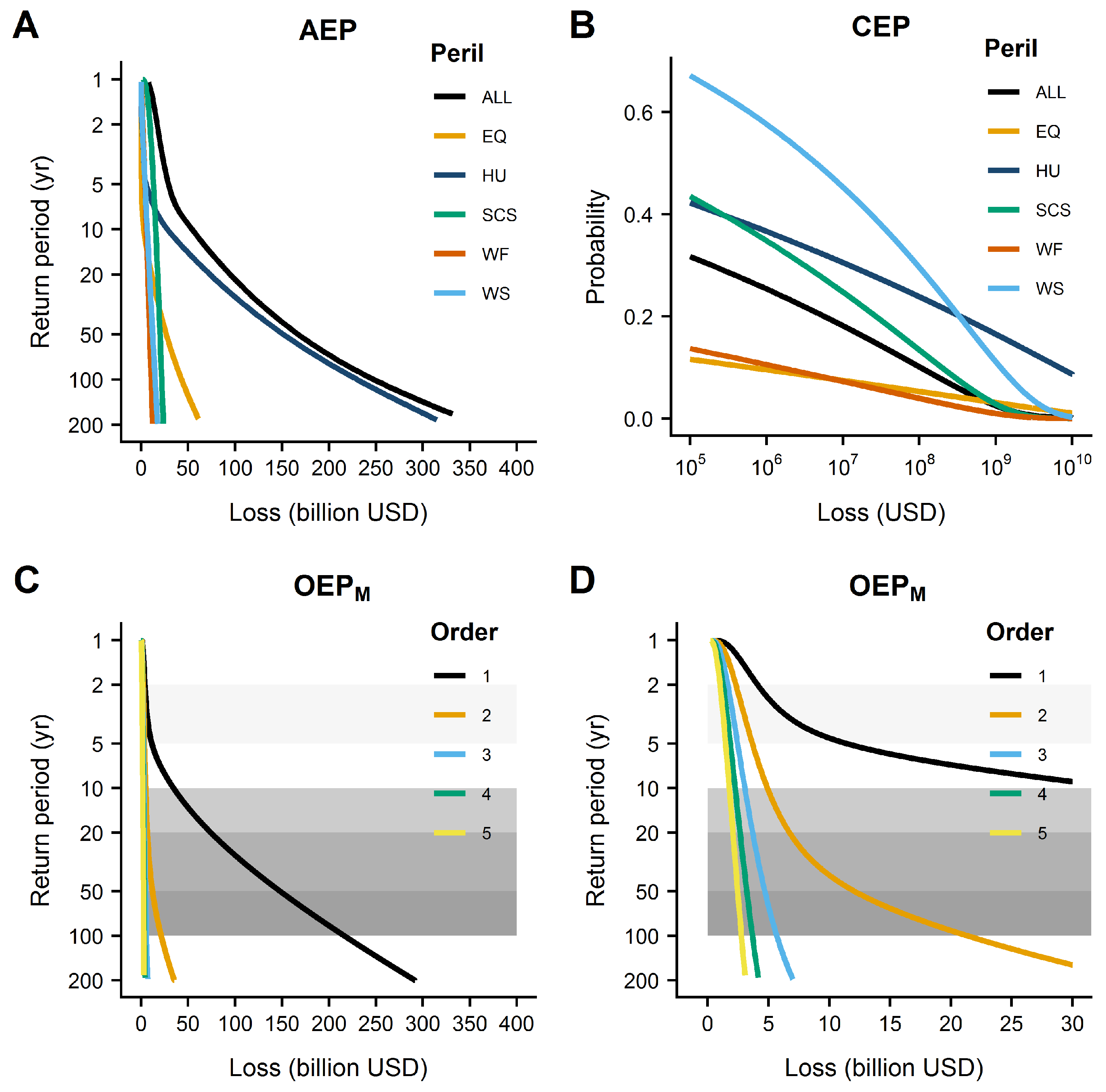
Figure 4 provides another viewpoint on the risk profile. Panel A of Figure 4 displays the annual aggregate loss exceedance probability (1 minus the cumulative probability, labeled as AEP) where the y-axis is displayed in terms of return period (1 over the exceedance probability) using a standard convention. Panel A makes clear the dominance of HU for tail risk in our multi-peril model. Panel A also demonstrates how SCS dominates short return periods (due to the relatively high AAL with high frequency), followed by WF and WS (the next two highest frequency perils). Panel A also shows that EQ is the second most important component of tail risk albeit a distant second compared to HU in our model. Panel B of Figure 4 displays the exceedance probabilities associated with the individual peril model severities (EQ, HU, SCS, WF and WS) as well as the mixture model for the multi-peril severity (ALL). Panel B re-iterates the idea that HU has the highest loss potential in our model. Panels C and D display the multi-peril exceedance probability curves for the occurrence losses $X_M$ for orders $M=1,2,3,4,5$ (obtained by integration using Equation (11), and labelled by OEPM). Panel D is a zoomed version of Panel C, and displays an intriguing set of relationships between the occurrence losses.

3.2. Pre-catXL Loss Decomposition for the Multi-Peril Case

Here we discuss in detail the decompositions of the AAL (Equation (3)), the annual aggregate loss variance (Equations (4) and (5)), and the correlation structure across occurrence losses (Equation (17)) for the pre-catXL perspective, setting the stage for our analysis of the post-catXL case to follow.

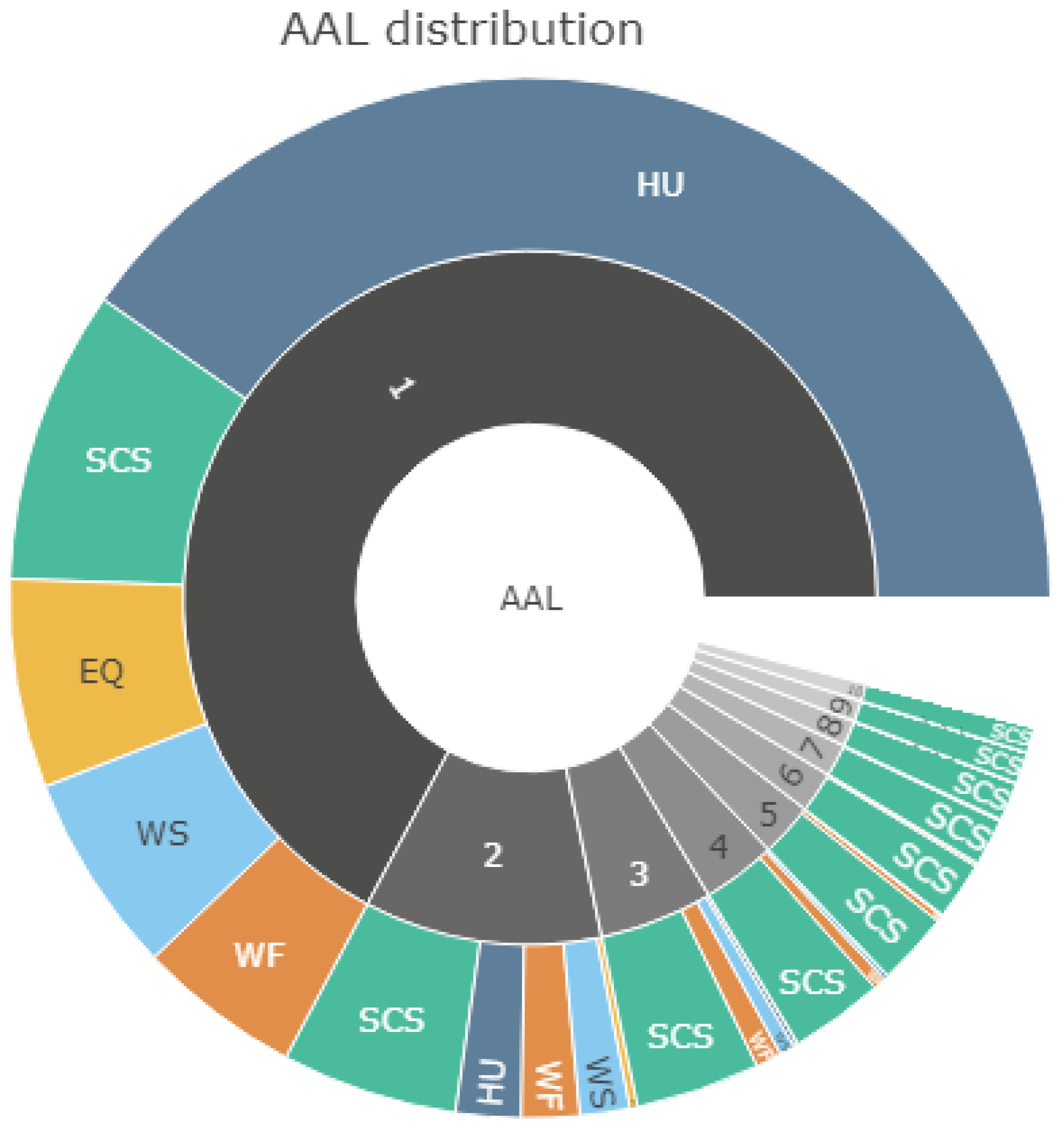
We begin with the decomposition of the pre-catXL AAL displayed in Figure 5. In Figure 5, the inner (gray shaded) circle represents, proportional to the arc length, the contribution from the different occurrence losses. The results are obtained by numerical integration using our analytical formulation in Equation (12) (where the normalizing factor $AA{L}_{pre}$ in Equation (3) is obtained using a $S=$ 500,000 year simulation procedure discussed in Appendix D). Note that in what follows we will address the accuracy of our numerical integration schemes versus brute force numerical simulation, but we leave that aside for the moment. Figure 5 is interesting for the following reasons. Firstly, we see that the order $M=1$ occurrence loss dominates the pre-catXL AAL with a roughly 60 percent contribution. Secondly, non-trivial contributions are made by orders $M=2,\dots ,10$, but very little contribution is made from occurrence losses $M=11$ and above. We have also used our $S=$ 500,000 simulation to further decompose the orders into the contributions from the individual perils (Appendix D makes clear how the peril contributions are quantified). This second level of decomposition sheds even further light on the nature of the results. Figure 5 makes clear that HU dominates the $M=1$ order, but there are non-trivial contributions from SCS, EQ, WS and WF. Order $M=2$ shows the diminishing importance of HU, and in fact SCS dominates with non-trivial contributions from HU, WF followed by WS. For orders $M=3$ and above, it is clear that SCS, due to its high frequency nature and large AAL (Table 1) dominates.

Table 2. Convergence errors in the mean annual losses for the pre-catXL perspective (in Figure 5) for various occurrence loss orders $M=1,\dots ,10$ using Equation (18). The first column has the occurrence loss order. The second column provides the number of simulation years ($S=1000=1K$ and $S={10}^6=1M$ years of simulation).

Order	S = 1K	S = 10K	S = 100K	S = 1M
1	8.5	2.69	0.85	0.27
2	5.7	1.8	0.57	0.18
3	2.35	0.74	0.24	0.07
4	1.62	0.51	0.16	0.05
5	1.51	0.48	0.15	0.05
6	1.49	0.47	0.15	0.05
7	1.5	0.47	0.15	0.05
8	1.52	0.48	0.15	0.05
9	1.55	0.49	0.15	0.05
10	1.58	0.50	0.16	0.05

displays estimates of convergence errors (in percentage terms) for the mean losses associated with all the orders $M=1,\dots ,10$ displayed in Figure 5. The errors in Table 2 are computed using Equation (18) (where the standard deviation is computed via numerical integration using the square root of Equation (14)). The implications of Table 2 are perhaps self-evident, but, our results indicate that catastrophe modeling systems based on $S=10K$ years of simulation can generate unacceptably large errors (few percent) in fundamentally important metrics like the mean annual loss associated with order $M=1$. Our results suggest that around $S=100K$ should be used to reduce errors in the various orders to below 1 percent. Our framework enables one to systematically investigate convergence errors (although not done here to limit scope). Finally, we note that percentage errors for higher order losses are lower than lower orders. This is not surprising as higher order losses have an enhanced likelihood of being assigned zero value (and therefore vary less than the annual maximum for example).

The mean loss results presented in Figure 5 (the inner grayscale circle segments) are obtained using Equations (3) and (12). For completeness, we have recorded the accuracy estimates associated with our numerical integration. We have used standard functions in Mathematica to perform the numerical integrals, with no explicit attempt to optimize the accuracy. Mathematica provides error estimates. Results for orders $M=1,2,3$ are presented in

Table 3. Numerical integration errors associated with the mean annual pre-catXL loss estimates for different orders (presented in Figure 5). Column 1 displays the occurrence loss order, and Column 2 gives the numerical integration errors for each pre-catXL mean loss estimate.

Order	Percentage Error
1	0.12
2	0.11
3	0.09

(in percentage terms). Table 3 shows that the percentage errors are well below 1 percent. Given the convergence errors presented in Table 2, we can loosely infer that our numerical integrals are as accurate as results from simulations of order $S=1M$ years. We are therefore confident that our numerical integrations are highly accurate.

Figure 6 displays the decomposition of the pre-catXL annual aggregate loss variance using Equations (4), (5), (12), (14) and (17). We again use the $S=$ 500,000 year simulation to estimate the total variance. The leading term is the marginal contribution from the order $M=1$ occurrence loss, followed by progressively smaller contributions from the 2/1 interaction term between $M=1$ and $M=2$, the marginal $M=2$ term, and the 3/1 interaction term. In contrast to Figure 5 for the AAL decomposition, the total variance structure is more strongly dominated by the order $M=1$ occurrence loss (well over 75% of total variance). Figure 6 also demonstrates the dominance of the order 1 occurrence loss through the appearance of the 2/1 and 3/1 interaction terms (as the second and fourth most important terms). The appearance of the interaction terms also points to the importance of the correlation structure across occurrence losses.

Analogous to Table 2, we have estimated the standard errors of the marginal and interaction terms contributing to the total variance, displayed in

Table 4. Convergence errors (in percentage terms) associated with the marginal and interaction terms for the pre-catXL total variance. Column 1 indicates the term (which is 1 for the $M=1$ marginal contribution, and Int 2/1 for the interaction term between $M=1$ and $M=2$). Similar to Table 2, results for $S=1K$ to $S=1M$ years of simulation are shown.

Order	S = 1K	S = 10K	S = 100K	S = 1M
1	4.47	1.41	0.45	0.14
Int 2/1	17.13	5.45	1.73	0.55
2	4.47	1.41	0.45	0.14
Int 3/1	30.42	9.65	3.05	0.97

. For example, for the marginal $M=1$ term in row 1 of Table 4, the percentage error for a $S=10K$ year simulation is approximately 1.41 percent. The standard errors for the marginal contributions are computed using Equation (19). For the interaction terms, we use Equations (20) and (21) to estimate the errors in the standard deviations and Pearson correlations. For both the marginal and interaction contributions, we have added up errors from individual terms in the required integrals using a standard method (University of Toronto 2021), under the assumption that errors are independent (which they are generally not). Furthermore, we note that our error estimate for the Pearson correlation is itself approximate (due to non-normality). Our interest is to get a feel for the errors and hence these approximations were deemed acceptable. For example, Table 4 indicates that well over $S=100K$ simulations are required to obtain percentage errors below 1 percent (for the leading terms that contribute to the total variance). Comparing Table 3 and Table 4 indicates the resolving the variance structure requires larger numbers of simulations than for the AAL.

Table 5. Numerical integration error estimates (in percentage terms) for various marginal and interaction terms involved in decomposing the pre-catXL total annual aggregate variance. Column 1 indicates the particular marginal or interaction term, and Column 2 indicates the percentage error.

Term	Percentage Error
1	0.11
2	0.17
3	0.48
Int 2/1	0.29
Int 3/1	0.70
Int 3/2	0.72

displays our estimates of numerical integration errors associated with the various marginal and interaction terms. Similar to Table 3, we have used output from Mathematica to estimate numerical integration errors of various terms involved in the computations, and used a standard method for adding up errors (University of Toronto 2021), again using the assumption of independence of errors. Table 5 again gives us a feel for the order of magnitude of errors arising from numerical integration. For example, Table 5 shows the percentage error associated with the $M=1$ marginal term is around 0.1 percent, and 0.29 percent for the 2/1 interaction term. Comparison of Table 5 with Table 4 shows that the numerical integration process has similar accuracy to running a $S=1M$ year simulation.

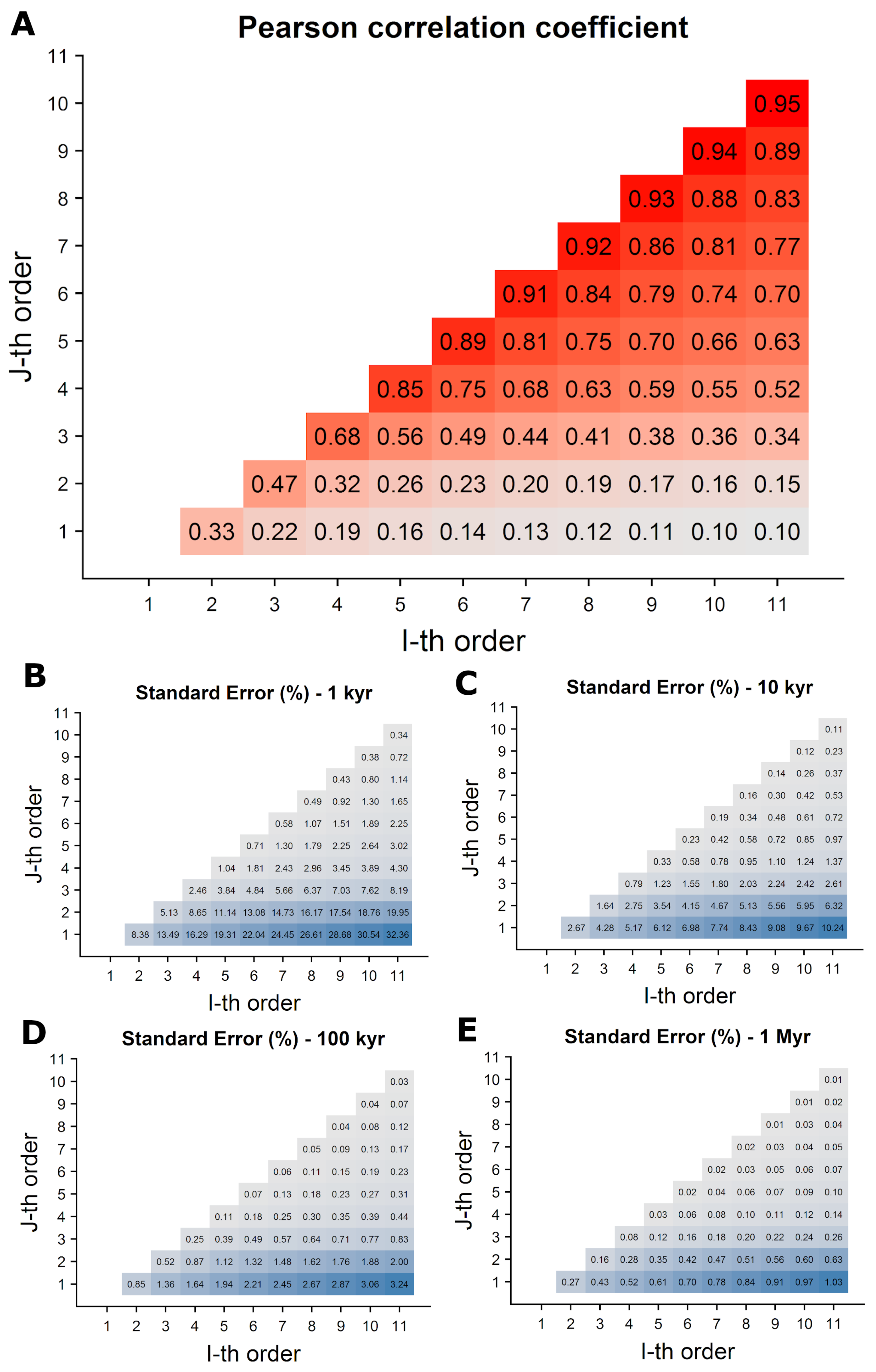
Figure 7 Panel A displays the correlation structure in the pre-catXL occurrence losses. The results in Figure 7 have been computed using Equation (17) via numerical integration. Figure 7 Panel A reveals a very interesting correlation structure. First, we note that higher order occurrence loss interactions have much higher correlation than lower order correlations. For example, the correlation between $M=1$ and $M=2$ is 0.33 (as seen in Panel A), and the correlation between $M=10$ and $M=11$ is approximately 0.95. Our explanation is that the higher order losses are more likely to be simultaneously small driving up correlation. Lower order losses can take on a large range of values, and this added variation leads to lower correlation. The bottom 4 panels of Figure 7 display convergence error estimates, in percentage terms, derived using our approximate standard error Equation (21). Our results indicate that order $S=1M$ years of simulation are required to achieve accuracy of better than 1 percent.

The following is a list of key results and conclusions derived from our analysis of the pre-catXL occurrence loss decompositions presented above:

• The order $M=1$ occurrence loss makes up roughly 60 percent of total AAL, with non-trivial contributions from occurrence losses $M=2,\dots ,10$. Using a $S=$ 500,000 year simulation, we have further decomposed each occurrence loss contribution into the individual peril contributions. At lower orders, HU is dominant, but, all other perils (SCS, EQ, WS and WF) make significant contributions. AAL contributions from higher order occurrence losses are dominated by SCS (with high frequency and significant AAL). Our calculations demonstrate that order $S=100K$ simulations are required to achieve less than 1 percent errors in the contributions from various occurrence loss orders, and we find that our numerical integration process is highly accurate, corresponding to roughly $S=1M$ years of simulations.
• The total variance structure is dominated by the marginal contribution from the order $M=1$ occurrence loss, followed by significant contributions from the marginal $M=2$ contribution, the 2/1 interaction term, and the $M=3$ marginal contribution. Relative to the AAL decomposition, the order $M=1$ occurrence loss is even more dominant, with an over 75 percent contribution to the total variance. Our calculations reveal that order $S=1M$ simulations are required to achieve accuracy of 1 percent or better, and our integration process was found to be highly accurate.
• Our analysis of the pre-catXL correlation structure across occurrence losses reveals an interesting structure, with lower order occurrence loss pairs being less correlated than higher order interaction terms. We find that order $S=1M$ years of simulation are required to achieve errors of less than 1 percent in the correlation structure.

We have now set the stage for our analysis of the post-catXL perspective where we will investigate how the characteristics of the decomposition change as the terms of the reinsurance contract changes. Our analysis will provide an understanding what aspects of our multi-peril model are important for various types of catXL layers covered by insurers and reinsurers.

3.3. Post-catXL Loss Decomposition for the Multi-Peril Case

Figure 8 displays post-catXL AAL results for 4 layers. In each case, we specify the attachment $\$A$ and exhaustion point $\$E$ using loss thresholds obtained from the $M=1$ occurrence loss distribution in Figure 4 Panel C (a common approach in practice). For example, in Figure 8 Panel A, the attachment point is the loss threshold associated with return period 1, and the exhaustion point is associated with return period 2. Typically, reinsurers will provide coverage for layers corresponding to higher return periods (Panels C and D) whereas lower layers are retained by insurers (Panels A and B).

Panel A in Figure 8 clearly demonstrates that the AAL is comprised of non-trivial contributions from occurrence losses up to order $M=10$. The inner grayscale decomposition in Panel A is obtained using numerical integration, but we have also used our $S=$ 500,000 year simulation (see Appendix D) to further decompose the results into the peril contributions (analogous to the pre-catXL case). Panel A demonstrates that the $M=1$ occurrence loss explains roughly 40 percent of the AAL (lower than in the pre-catXL case with 60 percent) while the most significant contributor is from SCS, followed by WS, WF, HU and EQ. For higher order contributions, SCS plays a progressively larger role in explaining the AAL. The contrast between Figure 8 Panel A and Figure 5 (pre-catXL AAL) is stark. The introduction of the catXL operator $t_{AE}\left(\right)$ in Panel A leads to more of an emphasis on the 3 highest frequency perils (SCS, WF and WS). HU and EQ play a smaller role in Panel A since losses happen infrequently, and when they do occur, the catXL operator $t_{AE}\left(\right)$ caps the severity of the loss. We note again that the lowest layers are typically the responsibility of primary insurers. Our results clearly demonstrate the importance of accurately modeling high frequency perils from the perspective of a primary insurer.

Panel B in Figure 8 shows AAL results for the 2–5 year return period layer. The $M=1$ occurrence loss now dominates the AAL with an over 90 percent contribution, the majority of which is derived from HU, followed by meaningful contributions from EQ, WS, SCS and WF. The results in Panel B are a stepping stone to the higher layers depicted in Panels C and D. Panels C and D show the dominance of the $M=1$ occurrence loss, which itself is dominated by HU, followed by EQ. The highest layers are dominated by low-frequency and high severity perils. The most extreme layer depicted in Panel D clearly demonstrates that the HU losses are almost singularly important when determining the AAL component of the catXL premium. While our results in Panel D would be well appreciated by market practitioners, our mathematical framework enables us to shed light on this result in a precise way.

Table 6. Convergence errors for various AAL results displayed in Figure 8 are provided for the $S=100K$ simulation years case. Column 1 provides the layer definition, Column 2 provides the occurrence loss order and Column 3 the percentage error. Results are analogous to the pre-catXL convergence errors displayed in Table 2.

Layer	Order	Percentage Error
1–2 year	1	0.09
1–2 year	2	0.13
1–2 year	3	0.15
1–2 year	4	0.15
1–2 year	5	0.15
10–20 year	1	1.08
10–20 year	2	5.39
10–20 year	3	30.92
10–20 year	4	199.64
10–20 year	5	1419.56

provides convergence errors for the results in Figure 8 for $S=100K$ simulation years, for a selection of layers and occurrence loss orders (computed in the same way as the pre-catXL case). Table 6 demonstrates very large standard errors for the higher order contributions to the 10–20 year return period layer. While these contributions are generally not significant, and negates to some degree their practical significance, Table 6 suggests the need for greater than $S=100K$ simulation years for accurate catXL technical pricing.

Table 7. Numerical integration errors associated with a selection of results in the post-catXL AAL decompositions provided in Figure 8. Column 1 provides the occurrence loss order (for the 1–2 return period layer) and Column 2 the percentage error.

Term (1–2 year)	Percentage Error
1	0.05
2	0.06
3	0.07

provides a selection of estimates of numerical integration errors for the order $M=1,2,3$ contributions to the 1–2 year return period layer. In comparison to Table 6, the results in Table 7 again demonstrates that our numerical integration process is highly accurate, and roughly corresponds to order $S=1M$ years of timeline simulation.

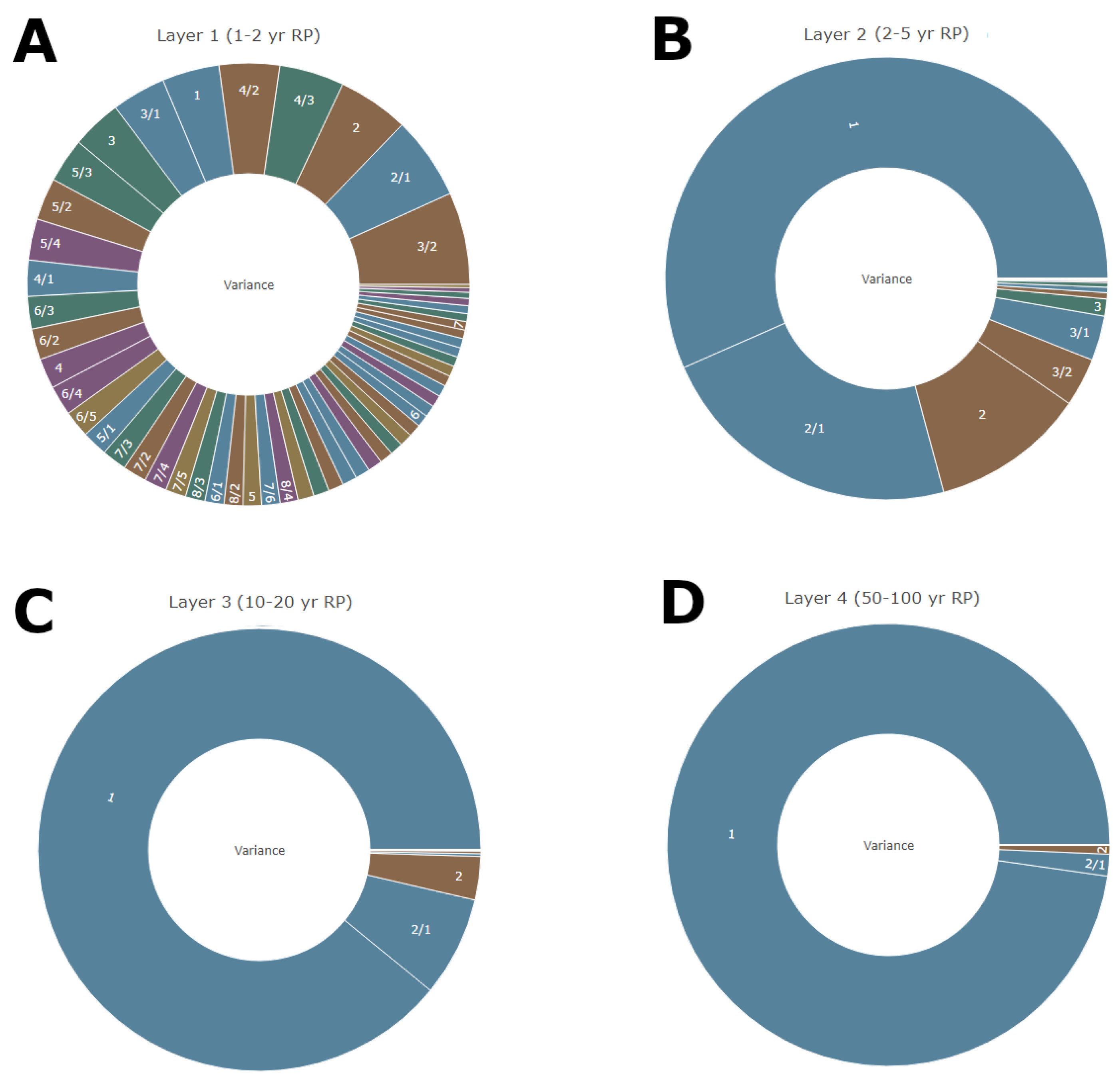
Figure 9 plots the variance decomposition for the 4 catXL layers of interest. Panel A of Figure 9, which shows results for the 1–2 year return period layer, depicts a rich structure with many interactions contributing to the total variance. The 3 largest contributors are the order 3/2 interaction, followed by the 2/1 interaction, and then the marginal contribution of the order 2 occurrence loss. The fact that the 3/2 interaction term is greater than the 2/1 interaction term could in part be explained by the higher correlation in the 3/2 term (0.78) versus the 2/1 term (0.65) (correlations are provided in Figure 10 to follow). The key takeaway from Panel A is that the variance is driven by a large set of interaction terms across the different orders, and modeling such interactions accurately is important for risk takers that provide coverage for such layers (primary insurers). Panel B of Figure 9, corresponding to the 2-5 year return period layer, shows a much less rich structure, which is dominated by the order 1 occurrence loss. As we move to progressively higher catXL layers in Panels C and D, the order 1 occurrence loss becomes nearly singularly important (explaining well over 90 percent of the total variance). Given our findings for the AAL depicted in Figure 8, this order 1 occurrence loss is largely attributable to HU. The results in Figure 9 for the total variance further bolster the notion that the HU peril dominates the pricing of high catXL layers in our particular multi-peril setup.

Table 8. A selection of post-catXL variance contribution term standard errors for $S=100K$ simulation years (corresponding to the results displayed in Figure 9). Column 1 provides the Layer, Column 2 provides the type of term, and Column 3 contains the percentage error.

Layer	Term	Percentage Error
1–2 year	Int 3/2	0.54
1–2 year	Int 2/1	1.73
1–2 year	2	0.45
1–2 year	Int 4/3	0.28
1–2 year	Int 4/2	0.69
10–20 year	1	0.45
10–20 year	Int 2/1	2.79
10–20 year	2	0.45
10–20 year	Int 3/1	16.2
10–20 year	Int 3/2	3.04

provides convergence errors, for $S=100K$, for the various (variance contribution) terms displayed in Figure 9 (using the same methodology as in the pre-catXL results provided in Table 4). Table 8 shows that most terms have standard errors below 1 percent, with the exception of interaction terms for the 10-20 year return period layer. While such terms do not explain a large part of the variance, our results nonetheless indicate that very precise quantification of all terms requires larger than $S=100K$ simulations. As noted in our discussion of the pre-catXL case, all terms in Table 8 are computed under assumptions which are not valid, but nonetheless give us a feel for the magnitude of the standard errors.

Table 9. Numerical integration errors for post-catXL annual aggregate variance decomposition. Column 1 indicates the various marginal and interaction terms for the 1–2 return period layer. Column 2 has the percentage error.

Term (1–2 year)	Percentage Error
1	1.58
2	0.93
3	0.84
Int 2/1	2.59
Int 3/1	2.53
Int 3/2	1.77

contains numerical integration errors we have computed using methods similar to those discussed for Table 5 in the pre-catXL case. Results in Table 9 are displayed for the 1–2 year return period layer. Table 9 shows that the numerical integration errors we have quantified are higher than the standard errors derived from a $S=100K$ year simulation (but not dramatically so). This was not the case in the analogous pre-catXL results, and it is not entirely clear why. Nonetheless, the results in Table 9 do demonstrate that the numerical integration process is accurate. We note once again the results in Table 9 are computed using assumptions which are not correct, but nonetheless give us a feel for the magnitude of the errors.

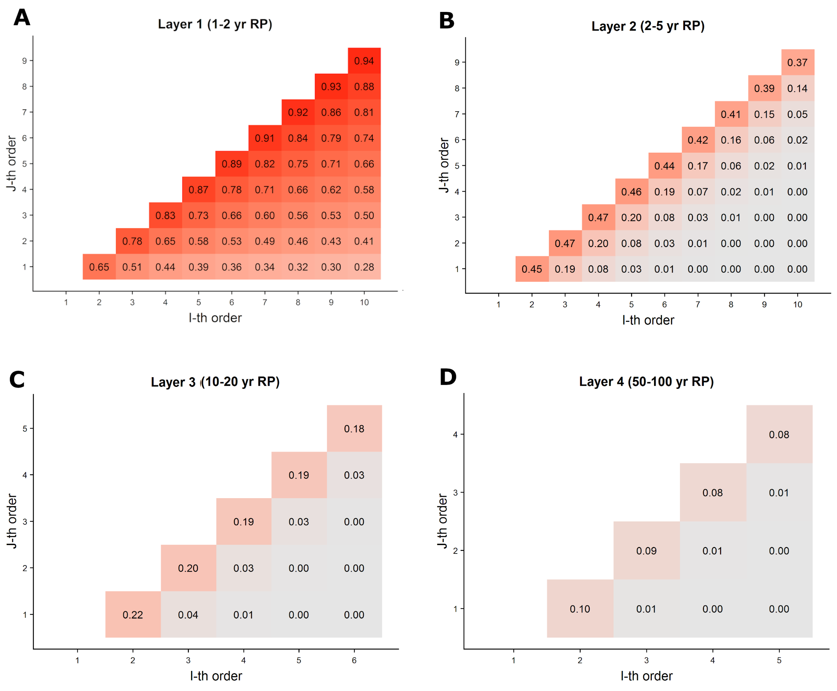
Figure 10 displays the correlation structures for the post-catXL results (computed using Equation (17) using the appropriate operator $t_{AE}\left(\right)$). Figure 10 shows that lower layers (Panels A and B) have strong correlations across the different occurrence loss orders, whereas the correlations drop to close to 0 for the highest layer in Panel D. This is a direct consequence of the effect of the catXL operator $t_{AE}\left(\right)$. For Layer 1, occurrence losses up to order 10 ‘survive’ the effect of $t_{AE}\left(\right)$, and are able to interact in a non-trivial way. For the highest Layer 4 in Panel D, higher order occurrence losses are nearly always zero due to the effect of $t_{AE}\left(\right)$, and the correlations as a consequence tend to 0. Comparing the results to the pre-catXL case is also interesting. For example, for Layer 1 in Figure 10, the correlations for the $(1/2,2/3,1/3)$ interaction terms are $(0.65,0.75,0.51)$ which is much higher that the pre-catXL equivalent set of correlations $(0.33,0.47,0.22)$. For the highest Layer 4 in Figure 10, the equivalent correlations are $(0.10,0.09,0.01)$, much lower that the pre-catXL results. We therefore infer that lower layers emphasize correlations across the occurrence losses, whereas the highest layers diminish their importance.

Our results for an idealized multi-peril catastrophe model for a US nationwide portfolio sheds light on interesting and different aspects of the occurrence losses. Our key findings are:

• For the lowest layers which are typically covered by primary insurers, we find non-trivial contributions from occurrence losses up to order 10 for the AAL. The decomposition of the variance clearly demonstrates that many interactions across occurrence losses are important, which is consistent with our results that strong correlations were found for interactions up to order 9. Due to the effect of the catXL operator $t_{AE}\left(\right)$, the AAL and total variance for the lowest layer have been shown to have the largest contributions from the highest frequency perils (SCS, WS, WF) and generally lower contributions from HU and EQ. As well, $t_{AE}\left(\right)$ increases correlation across all orders. The consequences in practical settings is that primary insurers must ensure accurate modeling of the higher frequency perils to achieve useful technical pricing for retained risk. Our mathematical framework sheds light on this in a precise way.
• The highest layers, typically covered by reinsurers, are dominated by the lowest frequency and highest severity perils (HU followed by EQ). What is perhaps surprising is the degree to which the maximum loss arising from hurricanes appears to dominate for the highest layer we have studied (50–100 year return period). The practical implications are clear that high layer catXL underwriters must pay careful attention to accurate modeling of HU. While this notion is well appreciated by market participants, our framework is able to quantify this in a precise way, and will enable practitioners to quickly assess the impact of different model assumptions on the decomposition of pricing metrics.

Within the context of our particular multi-peril catastrophe model, our results have made clear the importance of HU to the high layer reinsurance pricing problem. The following Section 4 uses a HU only model to address a question related to HU model adequacy.

4. Hurricane Model Sensitivity Results for a US Nationwide Portfolio

Section 3 makes clear the importance of HU to pricing the highest catXL layers typically covered by reinsurers. In this section, we study the sensitivity of the post-catXL loss decomposition to HU model assumptions. We are motivated by the following considerations: First, hurricane catastrophe models which are used in practice (Dong 2001; Katz 2002; Michel 2018; Mitchell-Wallace et al. 2017), oftentimes make a Poisson frequency distribution assumption (Katz 2002; Michel 2018; Mitchell-Wallace et al. 2017) as we have done in Section 3. Previous studies (Oxenyuk et al. 2017) of historical hurricane activity in the southeastern US, have shown the superiority of the Poisson frequency assumption as compared to the Negative Binomial assumption (using a variety of statistical tests). However, other studies have found that Florida landfalling hurricane activity is best modeled with frequency distributions that exhibit so-called clustered behavior (Jagger and Elsner 2012). The Negative Binomial distribution is an example of a clustered frequency model where the over-dispersion parameter $\frac{{\sigma }^2}{\mu }>1$ (using notation from Section 2.1.1). Furthermore, some reinsurance underwriters are of the opinion that current HU models under-represent potential losses from higher order occurrence losses, and that models should have more tunable parameters that influence the decomposition (Casey 2020). We also note that (Oxenyuk et al. 2017) finds that the historical data has an over-dispersion $\frac{{\sigma }^2}{\mu }\approx 1.23$. Given these motivating factors, we now examine the sensitivity of the post-catXL loss decomposition to the over-dispersion parameter.

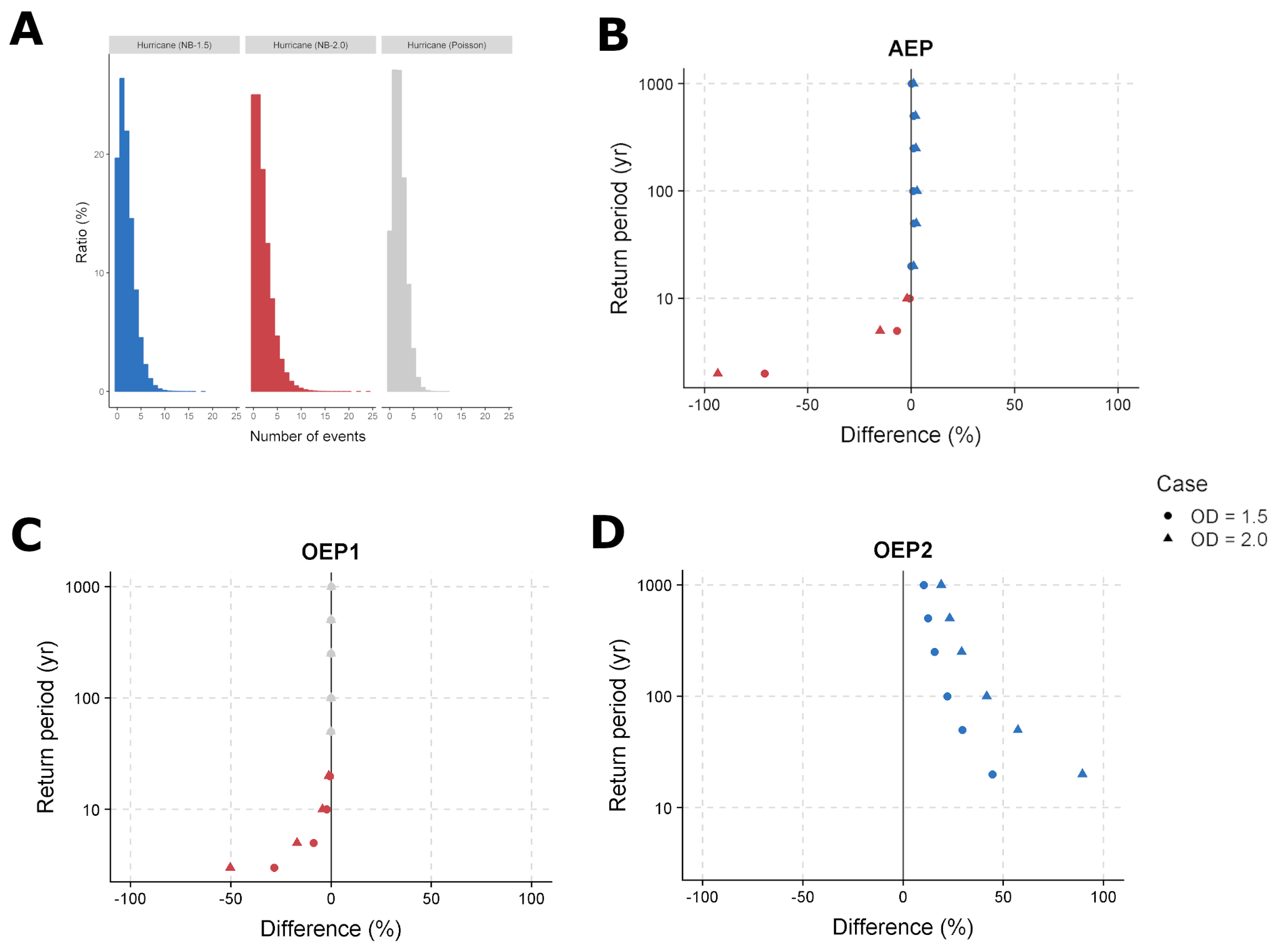
Our baseline HU model assumes a Poisson frequency with rate and severity parameters as in Table 1. We define two sensitivity models which instead use a Negative Binomial frequency distribution assumption with over-dispersion values of 1.5 and 2.0 (a reasonable upper bound sensitivity in light of the results in (Oxenyuk et al. 2017)), and with all parameters as in Table 1. The baseline and sensitivity models only differ in the frequency distribution choice. We first examine the basic risk profile displayed in Figure 11. Figure 11 Panel A depicts the discrete probability distributions for the two sensitivity models and the baseline model. The two sensitivity models exhibit higher probabilities of both small and high numbers of HU events. Figure 11 Panel B depicts the percent difference in the AEP of the two sensitivity models to the baseline model, showing large negative percentage differences at short return periods, and small positive differences at long return periods. Panels C and D depict the analogous percent difference plots for the order 1 and 2 occurrence loss distributions, respectively. Panel C shows how the over-dispersive models have negative differences at short return periods and converge to the baseline model at high return periods, whereas Panel D shows that the over-dispersive models are higher for the order 2 occurrence loss return period losses. The results in Panels C and D imply that the over-dispersive models have a lower contribution (to the AAL) from order 1, and a higher contribution from order 2, given that the AAL contribution (using Equations (6) and (13)) is proportional to the area under the exceedance probability curve.

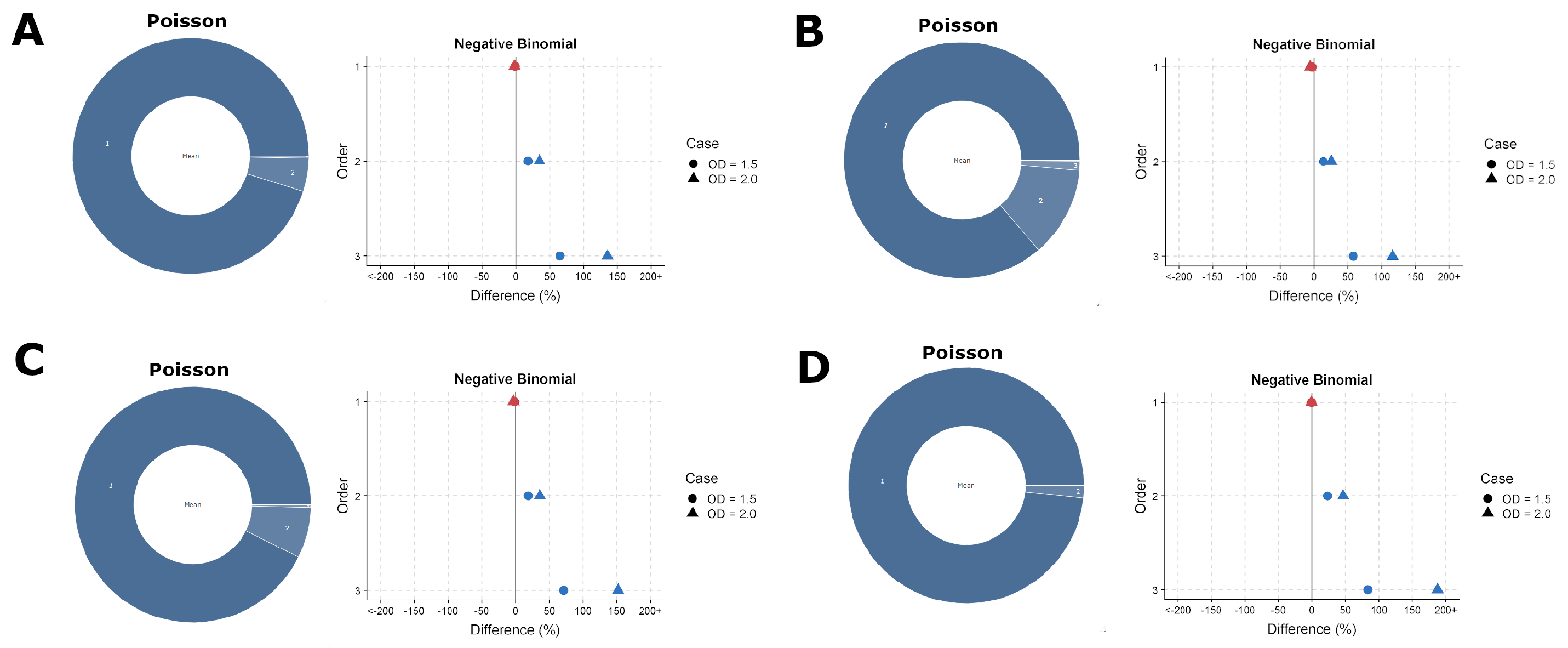
Figure 12 displays post-catXL AAL decomposition for 4 layers in Panels A, B, C and D. The attachment and exhaustion point loss thresholds are defined by the 1–2 year (Panel A), 2–5 year (Panel B), 10–20 year (Panel C) and 50–100 year (Panel D) return period loss thresholds derived from the baseline HU only Poisson order 1 occurrence loss distribution (similar approach to the multi-peril model). We once again use our $S=$ 500,000 year simulation to compute the total AAL. Figure 12 Panel A depicts results for the 1–2 year return period layer, with the base Poisson model decomposition depicted by the colored circle (analogous to the multi-peril case). The adjacent graph depicts the percent change in the contribution of the first 3 occurrence loss orders to the AAL. Contributions for the Negative Binomial case are computed using Equations (6), (10) and (13). Panel A shows that the addition of over-dispersion has a dramatic impact on the percent contribution of order 2 (25%). However, since the contribution of occurrence loss 2 itself is already small (less than 10%), the resulting decomposition is $not$ highly sensitive to this model assumption. Panels B, C and D for the higher layers tell the same story.

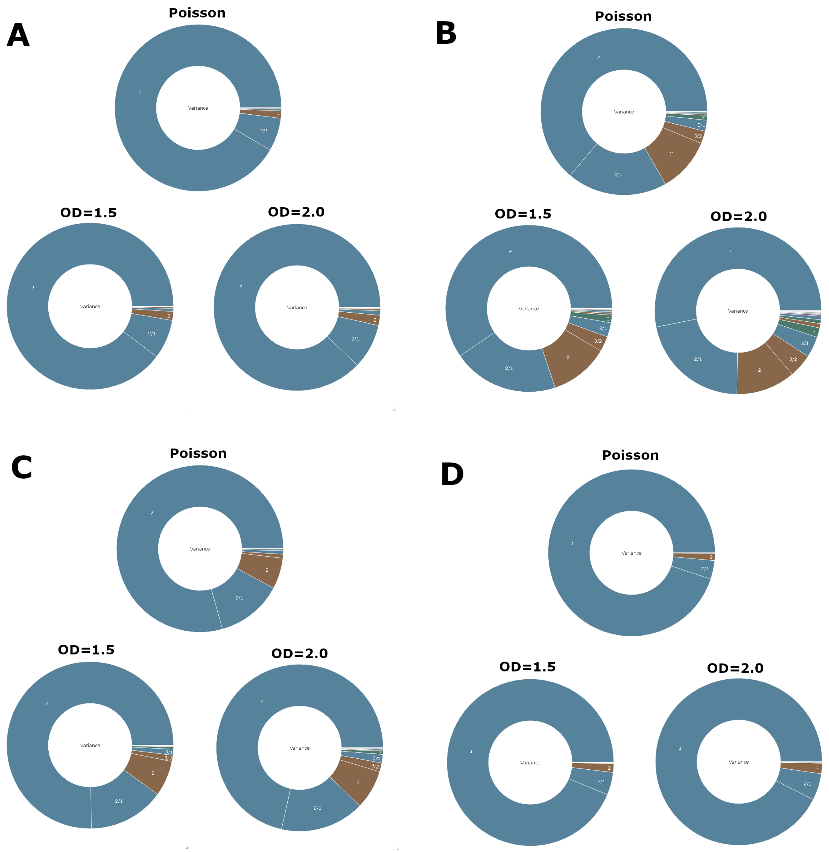
Figure 13 Panels A–D shows the decompositions of the total variance for the same layers depicted in Figure 12 (once again we use $S=$ 500,000 year simulation to compute total variance). Results for the Negative Binomial assumption (labelled by OD = 1.5 and OD = 2.0) are computed using Equations (10), (13), (15) and (16). Figure 13 (which shows the full decompositions as an alternative to Figure 12) makes clear that the inclusion of over-dispersion does not make a dramatic impact on the characteristics of the total variance decomposition.

We have computed numerical integration errors for terms depicted in Panels A of Figure 12 and Figure 13 (using the exact same methods discussed in Section 3). The results in

Table 10. Numerical integration errors for the post-catXL HU only results for various terms presented in Figure 12 and Figure 13 (analogous to Table 3, Table 5, Table 7 and Table 9). Column 1 indicates the particular mean or total variance statistic, Column 2 has the occurrence loss order (or interaction term) for the 1–2 year return period layer and Column 3 has the percentage error.

Statistic	Order/Term (1–2 year)	Percentage Error
Mean	1	1.7 $\times {10}^{-5}$
Mean	2	7.9 $\times {10}^{-6}$
Mean	3	7.0 $\times {10}^{-6}$
Variance	1	3.8 $\times {10}^{-5}$
Variance	2	2.0 $\times {10}^{-5}$
Variance	3	3.1 $\times {10}^{-5}$
Interaction	2/1	1.9 $\times {10}^{-4}$
Interaction	3/1	1.9 $\times {10}^{-4}$
Interaction	3/2	2.0 $\times {10}^{-4}$

demonstrate that the numerical integration process is highly accurate, with percentage errors less that $0.0002$. Table 10 demonstrates much higher accuracy compared to the multi-peril case (Table 3, Table 5, Table 7 and Table 9), which we attribute to the relative simplicity of the severity distribution in the HU only case.

Above we have investigated the sensitivity of the post-catXL loss decomposition to the use a frequency distribution that includes clustering (in the form of an over-dispersive Negative Binomial). Our results show that the decomposition of the post-catXL AAL and total variance is $not$ sensitive to fairly dramatic departures from the Poisson baseline assumption (having tested over-dispersion values of 1.5 and 2.0, which is $higher$ than the historical data would suggest (Oxenyuk et al. 2017)). At least within the context of our simplified HU model, we can rule out the use of an over-dispersive Negative Binomial to make a dramatic impact the characteristics of the decomposition, and would not necessarily be a useful parameter to tune in an underwriting practice if so desired. We leave open the possibility that more sophisticated approaches to modeling clustering (e.g., Khare et al. 2015), or more physically realistic approaches that take climate variability into account (e.g., Villarini et al. 2012), or changes to the severity distribution, would result in larger changes to the characteristics of the decomposition, which may be desirable so that models can be tuned for applications (Casey 2020). In any case, we have demonstrated the utility of our mathematical framework for addressing these important sensitivities.

5. Summary and Conclusions

We have developed a mathematical framework to quantify the role that occurrence losses (order statistics (Barakat and El-Shandidy 2015; Buhrman 1973; Consul 1984; David and Nagaraja 2003; Gupta and Gupta 1984; Raghunandanan and Patil 1976; Young 1970)) play in catXL reinsurance pricing metrics. Our framework is comprised of:

• A general expression for the marginal distribution of a given occurrence loss random variable (Equation (9))
• General expressions for the occurrence loss marginal distributions applied to a Poisson and Negative Binomial frequency assumption (Equations (11) and (10))
• The mean loss attributable to a given occurrence loss random variable both before and after the application of a catXL contract (Equations (12) and (13))
• The variance attributable to a given occurrence loss random variable both before and after the application of a catXL contract (Equations (14) and (15))
• The Pearson correlation structure for occurrence losses both before and after the application of a catXL contract for the Poisson and Negative Binomial cases (Equations (17) and (16))

The mathematical results, which are summarized in Section 2 and derived in detail in the Appendices, can be used to decompose the average annual loss and total annual aggregate loss variance (key statistics used in pricing catXL contracts) into contributions from different occurrence losses both before and after the application of a catXL contract. Our framework enables us to answer important questions related to the role of various occurrence losses that arise in practice.

We have applied our framework to an idealized multi-peril model in Section 3, and a hurricane-only model in Section 4 (for a US nationwide exposure). The multi-peril model was designed to simulate losses arising from hurricanes, earthquakes, winter storms, severe convective storms and wildfires. Both the multi-peril and hurricane only model are derived using actual historical loss data, and were therefore deemed as an appropriate testbed. The key learnings were:

• In the multi-peril pre-catXL case: The AAL has non-trivial contributions from occurrence losses up to order 10, and the order 1 loss is dominated by hurricane, whereas the higher order losses are dominated by the high frequency severe convective storm peril. The variance decomposition is dominated by the order 1 marginal contribution, with non-trivial contributions from order 2 and the 2/1 and 3/1 interaction terms.
• In the multi-peril post-catXL case: The lower layers have contributions from many occurrence loss orders, and the contributions themselves are dominated by the highest frequency perils (such as severe convective storms, winter storm and wildfire). Relative to the pre-catXL case, the inclusion of a low layer catXL operator drives up correlation amongst the various post-catXL occurrence losses. The highest layers are dominated by hurricane (followed by earthquake). The inclusion of high layer catXL operators drives down correlation relative to the pre-catXL case. The application of our framework to the multi-peril case reinforces the notion, in a precise way, that risk takers covering lower layers must be concerned by a multitude of perils, and in particular the highest frequency perils, whereas those covering the highest layers should be most concerned with hurricane followed by earthquake.
• The application of our framework requires numerical integration, which after applying standard and non-optimized integration packages we have found to be highly accurate, and in nearly all cases equivalent to running one million years of simulation
• In the hurricane only post-catXL case: The role that various occurrence losses play in catXL pricing metrics is not sensitive to the addition of clustering to the model (modeled using an over-dispersive Negative-Binomial frequency distribution). Our results suggest that other types of model changes would be required to make a significant impact.

We hope our framework will enable practitioners in the market to understand the role of occurrence losses in catXL pricing metrics, and quickly test the sensitivity to changes in model assumptions. This could be done by using vendor catastrophe model output to fit baseline frequency and severity distributions, and in turn perturbing around this baseline. We end by discussing several new research directions which arise from this paper:

• Our mathematical framework uses an assumption of unlimited re-instatements (for mathematical convenience). Future work could address how the characteristics of the decomposition change with the inclusion of more complex contracts used in practice (using numerical simulations).
• Climate change is expected to impact catastrophe peril severity and frequency (e.g., see Knutson et al. 2020). Our framework can be used to assess the impact of a changing climate on the role that occurrence losses play in reinsurance pricing metrics.
• In practice, full physically-based catastrophe simulation models are not always used, even for some material perils such as severe convective storm. Instead, frequency and severity distributions are fit to historical data. This raises the question of how sensitive the occurrence loss decomposition is to uncertainty in this fitting process, and whether or not this could lead to mis-pricing in the market. Our framework can be used to study this problem.
• In the multi-peril setting, we have used numerical simulations to further decompose the various occurrence loss contributions into the the various perils (see Appendix D). Performing such calculations analytically appears to be an extremely challenging mathematical problem, and is left to future work.
• We have used our mathematical framework to quantify convergence errors that may arise in practical catastrophe model applications. Further work could explore the use of more advanced simulation techniques to improve convergence errors for a fixed computational cost (e.g., using surrogate models or machine learning).
• It appears possible to extend our mathematical framework to the retrocession (retro) reinsurance pricing problem (where a further catXL operator is applied the post-catXL perspective for many layers combined). Further research into this may yield insights into various aspects of occurrence losses and retro reinsurance technical pricing.
• Our framework has been presented for the case where we have assumed independence between frequency and severity. Recent work in an insurance context has explored the implications of this dependency (Peng et al. 2015). In a catastrophe modeling context, there are a number of perils where frequency and severity are dependent (e.g., flood). Future work could explore the extension of our framework to this case.
• We have presented numerical results for a hypothetical US industry portfolio. The insights we have developed are therefore conditional on this choice. Future work could explore the extension of our framework to other portfolio and peril combinations to yield new insights.
• In Section 4 we have explored the sensitivity of US hurricane results to the frequency distribution assumption. Other types of sensitivities are of interest from a practical and theoretical point of view and can be explored in future studies.

References

1. AON Thought Leadership. 2021. Available online: http://thoughtleadership.aon.com/Documents/20200122-if-natcat2020.pdf?utm_source=ceros&utm_medium=storypage&utm_campaign=natcat20 (accessed on 20 January 2021).
2. Bahnemann, David. 2015. Distributions for Actuaries. CAS Monograph Series 2: 1–200. [Google Scholar]
3. Barakat, Haroon Mohamad, and Mouhamed A. El-Shandidy. 2004. Order statistics with random sample size. International Journal of Statistics LXII: 233–46. [Google Scholar]
4. Buhrman, J. M. 1973. On order statistics when the sample size has a binomial distribution. Statistica Neerlandica 27: 125–26. [Google Scholar] [CrossRef]
5. Casey, Alex. 2020. Hiscox Reinsurance, London, UK. Personal communication.
6. Congressional Research Service. 2021. Available online: https://fas.org/sgp/crs/misc/IF10244.pdf (accessed on 20 January 2021).
7. Consul, Prem C. 1984. On the distributions of order statistics for a random sample size. Statistica Neerlandica 38: 249–56. [Google Scholar] [CrossRef]
8. Cummins, John David, Christopher M. Lewis, and Richard Phillips. 1999. Pricing excess-of-loss reinsurance contracts against catastrophic loss. In The Financing of Catastrophe Risk. Edited by Kenneth A. Froot. Chicago: University of Chicago Press, pp. 93–148. [Google Scholar]
9. David, Herbert A., and Haikady N. Nagaraja. 2003. Order Statistics, 3rd ed. Hoboken: Wiley and Sons. [Google Scholar]
10. Dong, Weimin M. 2001. Building a More Profitable Portfolio: Modern Portfolio Theory with Application to Catastrophe Insurance. London: Reactions Publications. [Google Scholar]
11. EECS. 2021. Available online: https://web.eecs.umich.edu/~fessler/papers/files/tr/stderr.pdf (accessed on 20 January 2021).
12. Ekheden, Erland, and Ola Hossjer. 2014. Pricing catastrophe risk in life (re) insurance. Scandinavian Actuarial Journal 4: 352–67. [Google Scholar] [CrossRef]
13. Fisher, Ronald Aylmer. 1915. Frequency distribution of the values of the correlation coefficient in samples of an indefinitely large population. Biometrika 10: 507–21. [Google Scholar] [CrossRef]
14. Fisher, Ronald Aylmer. 1921. On the probable error of a coefficient of correlation deduced from a small sample. Metron 1: 3–32. [Google Scholar]
15. Gershenfeld, Neil. 1998. The Nature of Mathematical Modelling, 1st ed. Cambridge: Cambridge University Press. [Google Scholar]
16. Gupta, D., and Ramesh C. Gupta. 1984. On the distribution of order statistics for a random sample size. Stastistica Neerlandica 38: 13–19. [Google Scholar] [CrossRef]
17. Hurlimann, Werner. 2005. Excess of loss reinsurance with reinstatements revisited. ASTIN Bulletin 35: 211–38. [Google Scholar] [CrossRef] [Green Version]
18. Insurance Information Institute. 2021. Available online: https://www.iii.org/fact-statistic/facts-statistics-us-catastrophes (accessed on 20 January 2021).
19. Jagger, Thomas H., and James B. Elsner. 2012. Hurricane clusters in the vincinity of Florida. Journal of Applied Meteorology and Climatology 51: 869–77. [Google Scholar] [CrossRef]
20. Katz, Richard W. 2002. Stochastic modeling of hurricane damage. Journal of Applied Meteorology 41: 754–62. [Google Scholar] [CrossRef] [Green Version]
21. Klugman, Stuart A., Harry H. Panjer, and Gordon E. Willmot. 2008. Loss Models: From Data to Decisions, 3rd ed. Hoboken: Wiley and Sons. [Google Scholar]
22. Khare, Shree, Alessandro Bonazzi, Christos Mitas, and Steve Jewson. 2015. Modelling clustering of natural hazard phenomena and the effect on re/insurance loss perspectives. Natural Hazards Earth System Sciences 15: 1357–70. [Google Scholar] [CrossRef] [Green Version]
23. Knutson, Thomas, Suzana J. Camargo, Johnny C. L. Chan, Kerry Emanuel, Chang-Hoi Ho, James Kossin, Mrutyunjay Mohapatra, Masaki Satoh, Masato Sugi, Kevin Walsh, and et al. 2020. Tropical cyclones and climate change assessment: Part II: Projected response to anthropogenic warming. BAMS 101: 302–22. [Google Scholar] [CrossRef]
24. Mata, Ana J. 2000. Pricing excess of loss reinsurance with reinstatements. ASTIN Bulletin 20: 349–68. [Google Scholar] [CrossRef] [Green Version]
25. Michel, Gero. 2018. Risk Modelling for Hazards and Disasters, 1st ed. Amsterdam: Elsevier. [Google Scholar]
26. Mitchell-Wallace, Kristen, Matthew Jones, John Hillier, and Matthew Foote. 2017. Natural Catastrophe Risk Management and Modelling, 1st ed. Hoboken: Wiley Blackwell. [Google Scholar]
27. Oxenyuk, Victoria, Sneh Gulati, B. M. Golam Kibriar, and Shahid Hamid. 2017. Distribution fits for various parameters in the Florida public hurricane loss model. Journal of Modern and Applied Statistical Methods 16: 481–97. [Google Scholar] [CrossRef] [Green Version]
28. Peng, Shi, Xiaoping Feng, and Anastasia Ivantsova. 2015. Dependent frequency-severity modeling of insurance claims. Insurance: Mathematics and Economics 64: 417–28. [Google Scholar]
29. Raghunandanan, Kannan, and S. A. Patil. 1976. On order statistics for random sample size. Statistica Neerlandica 26: 121–26. [Google Scholar] [CrossRef]
30. Rao, Calyampudi Radhakrishna. 1973. Linear Statistical Inference and Its Applications, 2nd ed. Hoboken: Wiley and Sons. [Google Scholar]
31. University of Toronto. 2021. Available online: https://faraday.physics.utoronto.ca/PVB/Harrison/ErrorAnalysis/Propagation.html (accessed on 20 January 2021).
32. Villarini, Gabriele, Gabriel A. Vecchi, and James A. Smith. 2012. U.S. landfalling and north Atlantic hurricanes: Statistical modeling of their frequencies and ratios. Monthly Weather Review 140: 44–62. [Google Scholar] [CrossRef] [Green Version]
33. Wasserman, Larry A. 2004. All of Statistics, 1st ed. New York: Springer. [Google Scholar]
34. Young, D. H. 1970. The order statistics of the negative binomial distribution. Biometrika 57: 181–86. [Google Scholar] [CrossRef]
Figure 1. A depiction of a timeline simulation for a given combination of frequency and severity. Each simulation period is one-year in length (x-axis). The y-axis is the primary insurer portfolio loss in $, before the application of any reinsurance. The annual maximum loss events are depicted by the 1’s with red circles. Second annual maximum losses are indicated by the 2’s with yellow circles and so on. Event losses that are less than or equal to $X < $A have values in the closed interval from $0 to $X. The dashed red and blue lines indicated by the $A and $E values correspond to the attachment and exhaustion point of a catXL reinsurance contract that will be applied in what follows.
Risks 09 00052 g001
Figure 2. This picture illustrates the application of a catXL contract to the pre-catXL timeline simulation depicted in Figure 1. Occurrence losses in Figure 1 below the attachment point are given $0 value. Occurrence losses greater than or equal to the attachment point, but less than the exhaustion point, are equal to the assigned value in Figure 1, minus the attachment point. All occurrence losses above the exhaustion point in Figure 1 are assigned a value of $(E-A). In all simulation years, all higher order occurrence losses which are not depicted are assigned $0 value.
Risks 09 00052 g002
Figure 3. This figure displays results from a S = 500,000 year timeline simulation derived from the multi-peril frequency and severity model. The first 5 set of results displays annual aggregate losses for WS, WF, SCS, HU and EQ. The colored dots represent the annual aggregate losses overlaid by a bar indicating the minimum, maximum, median and interquartile ranges. A histogram is also provided for each peril. The final set of results labelled ALL displays the analogous results for all of the 5 perils aggregated together.
Risks 09 00052 g003
Figure 4. (Panel A) depicts the AEP for the individual peril models, as well as the multi-peril model denoted by ALL. (Panel B) depicts the exceedance probability of the individual severity distributions, as well as the multi-peril model. (Panels C,D) depict the exceedance probability curves for the occurrence loss marginal distributions up to order M = 5 .
Risks 09 00052 g004
Figure 5. The decomposition of the pre-catXL AAL. The inner gray shaded circle displays (in proportion to the arc length) the contributions of the various occurrence loss orders to the full AAL. The color shaded segments with associated peril name abbreviations displays the contributions, to each occurrence loss order, of the individual perils. For example, the contribution of HU to order M = 1 is over 50 percent.
Risks 09 00052 g005
Figure 6. Here the variance decomposition of the pre-catXL total annual aggregate loss variance is displayed. The largest contribution comes from the marginal contribution of the order M = 1 occurrence loss, followed by the 2/1 interaction term, the marginal order 2 term, and the 3/1 interaction term.
Risks 09 00052 g006
Figure 7. (Panel A) displays the pre-catXL correlation structure across the occurrence losses up to order M = 11 . The (Panels BE) depict the convergence error estimates for S = 1 K , S = 10 K , S = 100 K and S = 1 M years.
Risks 09 00052 g007
Figure 8. (Panel A) depicts the AAL decomposition for a catXL layer with attachment and exhaustion points defined by the loss thresholds of the M = 1 occurrence loss distribution (Figure 4 Panel C) for the 1 and 2 year return periods, respectively. The results displayed here are analogous to the pre-catXL results in Figure 5. (Panels BD) show results for layers defined by return periods 2–5, 10–20 and 50–100 years, respectively.
Risks 09 00052 g008
Figure 9. (Panels AD) depict the post-catXL variance decomposition for the multi-peril model. The contribution of any particular marginal or interaction term is proportional to the arc length.
Risks 09 00052 g009
Figure 10. (Panel A) depicts the post-catXL correlation structure for Layer 1 (1–2 year return period). (Panels BD) depicts the correlation structure for Layers 2–4.
Risks 09 00052 g010
Figure 11. (Panel A) depicts discrete frequency distributions for the Poisson and two over-dispersive sensitivity models. (Panel B) depicts percent differences in the AEP relative to the Poisson baseline, and (Panels C,D) have the analogous results for the order M = 1 and M = 2 distributions.
Risks 09 00052 g011
Figure 12. (Panels AD) depict post-catXL AAL decomposition results for the 1–2, 2–5, 10–20 and 50–100 year return period layers. The over-dispersive sensitivity models are depicted by the x-y plots which give the percent change over for contributions up to order M = 3 relative to the baseline Poisson model.
Risks 09 00052 g012
Figure 13. Analogous results to Figure 12 are shown for the variance decomposition. Here the full decompositions are displayed, and demonstrates the insensitivity to prescribed changes in the frequency distribution.
Risks 09 00052 g013