Author Contributions
Conceptualization, Y.A. and S.W.I.; methodology, S.W.I.; software, Y.A.; validation, Y.A., S.W.I., and R.S.; formal analysis, Y.A., S.W.I., and R.S.; investigation, Y.A.; resources, Y.A. and S.W.I.; data curation, Y.A.; writing—original draft preparation, Y.A.; writing—review and editing, S.W.I. and R.S.; visualization, Y.A.; supervision, S.W.I. and R.S.; project administration, S.W.I.; funding acquisition, S.W.I. and R.S. All authors have read and agreed to the published version of the manuscript.
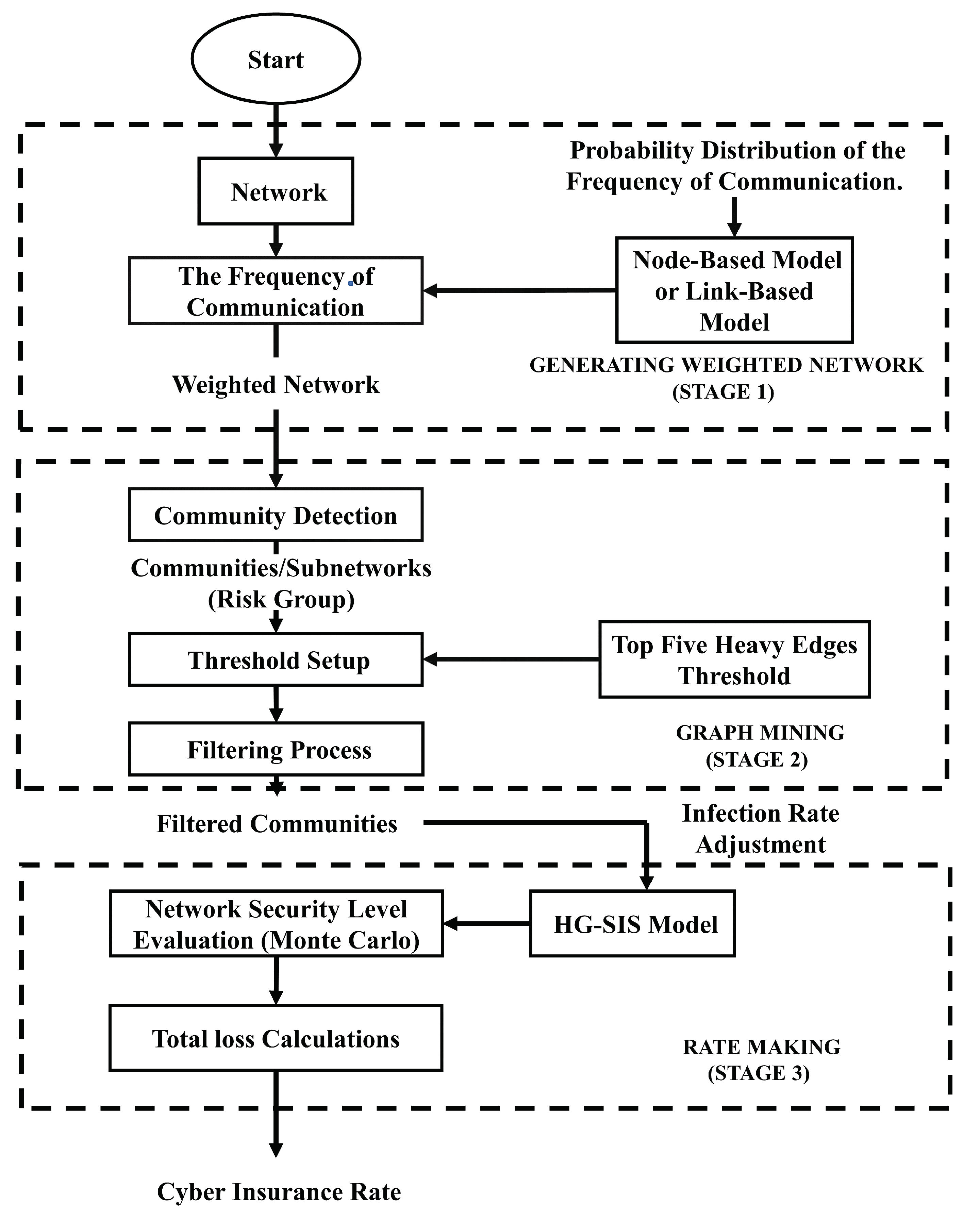
Figure 1.
Graph mining approach (GMA) used for cyber insurance ratemaking (CIRM).
Figure 1.
Graph mining approach (GMA) used for cyber insurance ratemaking (CIRM).
Figure 2.
An analogy based on a co-product purchases network used in market basket analysis to generate a communication network in the node-based model.
Figure 2.
An analogy based on a co-product purchases network used in market basket analysis to generate a communication network in the node-based model.
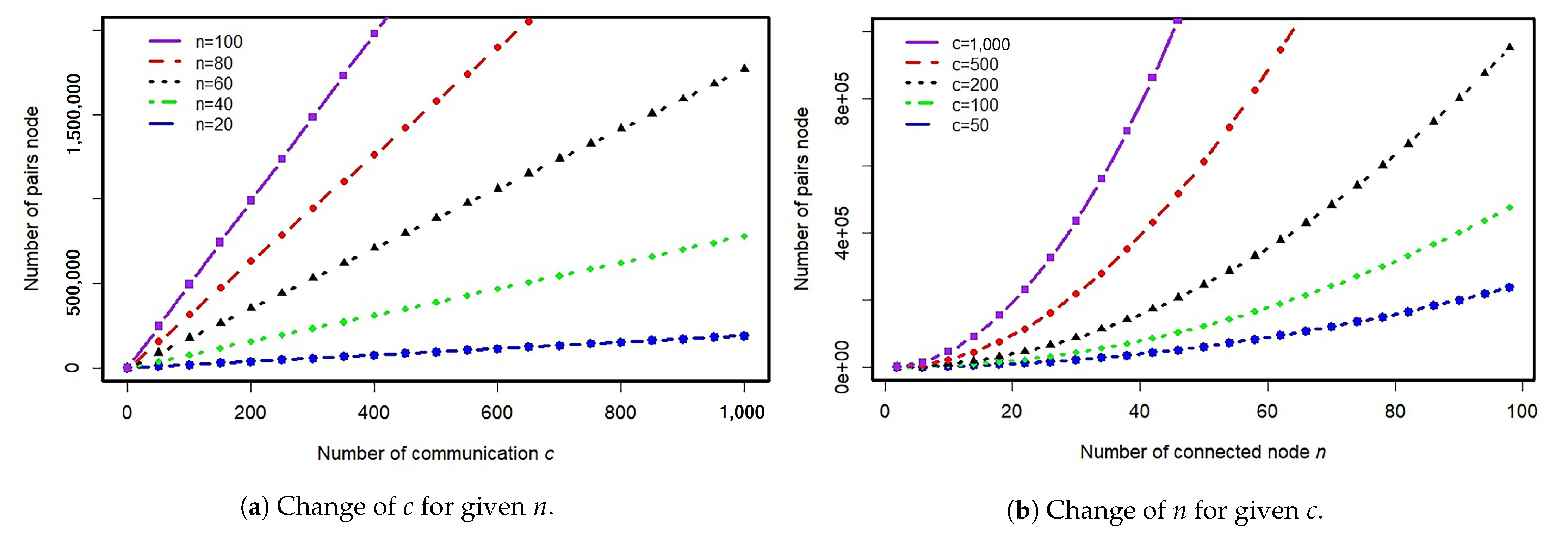
Figure 3.
Effect of c and n on the number of communications in the network during a day. (a) Change in c for a given n. (b) Change in n for a given c.
Figure 3.
Effect of c and n on the number of communications in the network during a day. (a) Change in c for a given n. (b) Change in n for a given c.
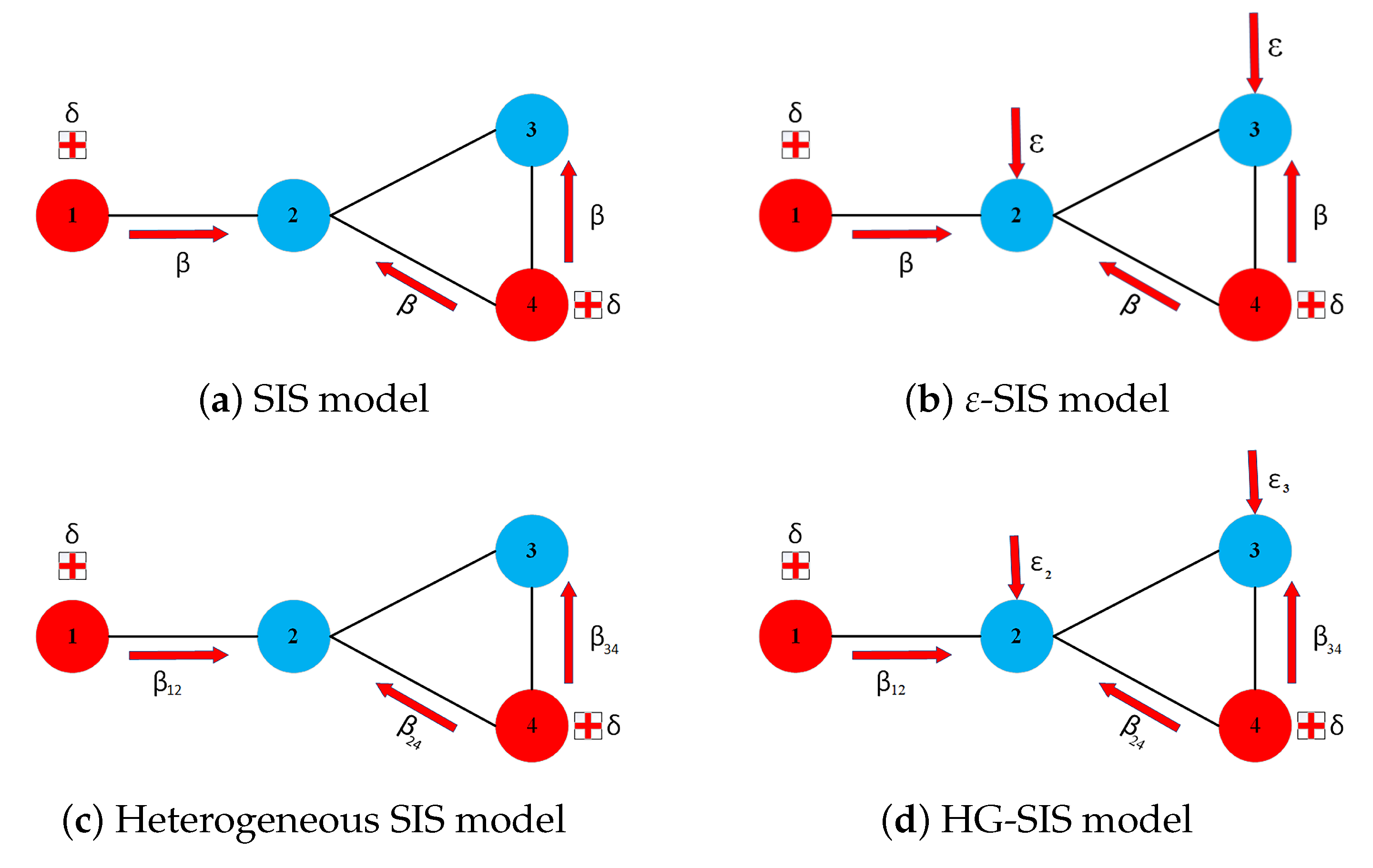
Figure 4.
Illustration for the difference in the SIS model, -SIS model, heterogeneous SIS model, and HG-SIS model in the node-level framework. (a) SIS model. (b) -SIS model. (c) Heterogeneous SIS model. (d) HG-SIS model.
Figure 4.
Illustration for the difference in the SIS model, -SIS model, heterogeneous SIS model, and HG-SIS model in the node-level framework. (a) SIS model. (b) -SIS model. (c) Heterogeneous SIS model. (d) HG-SIS model.
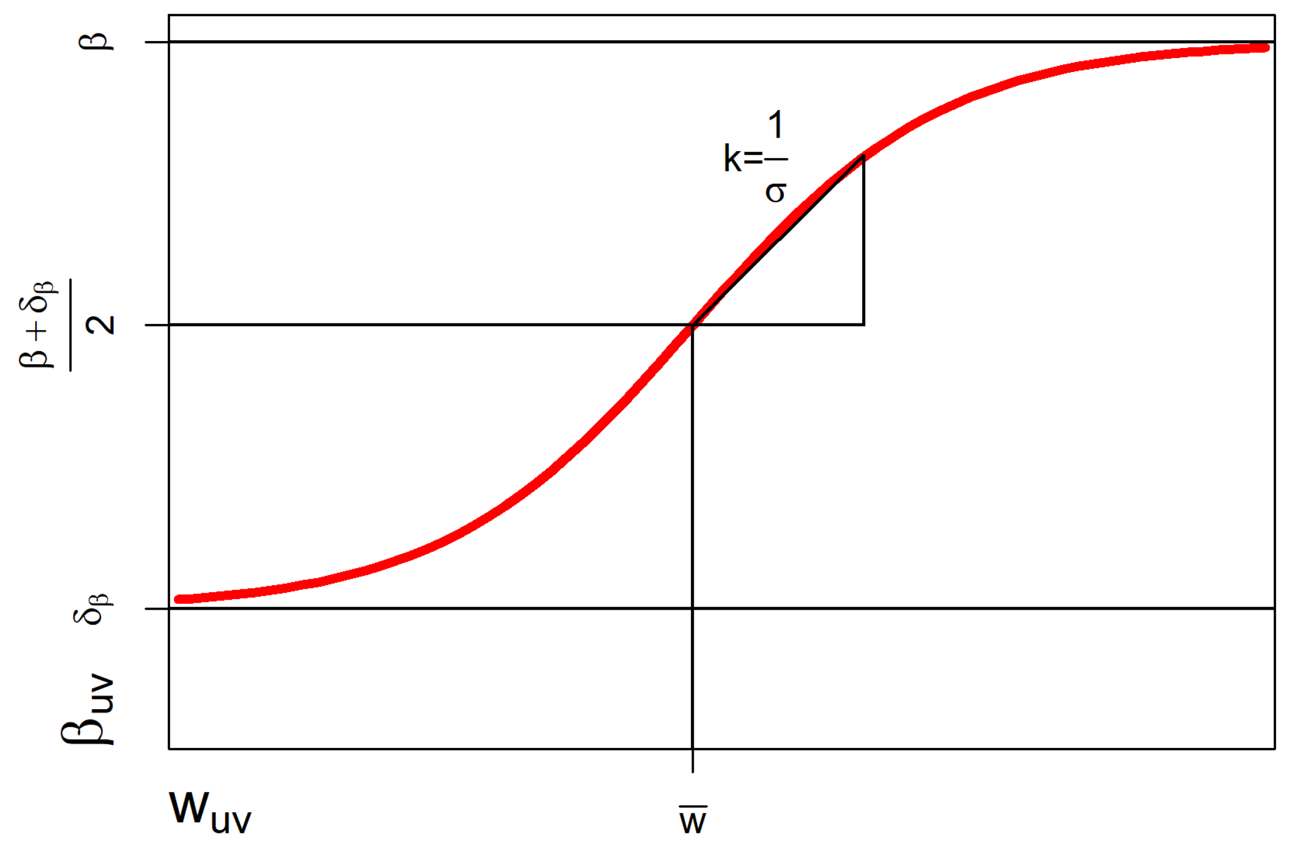
Figure 5.
Transformation function for in the range using communication weight .
Figure 5.
Transformation function for in the range using communication weight .
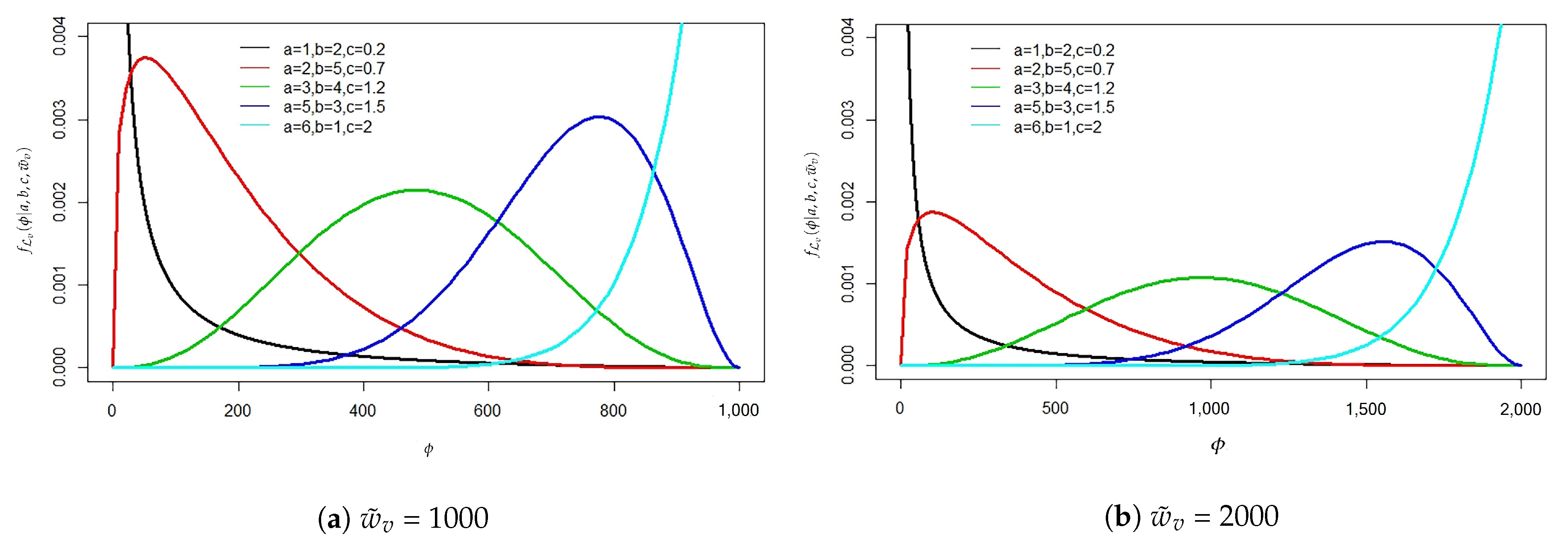
Figure 6.
Profile of losses caused by infection following a generalized beta distribution for the given parameters.
Figure 6.
Profile of losses caused by infection following a generalized beta distribution for the given parameters.
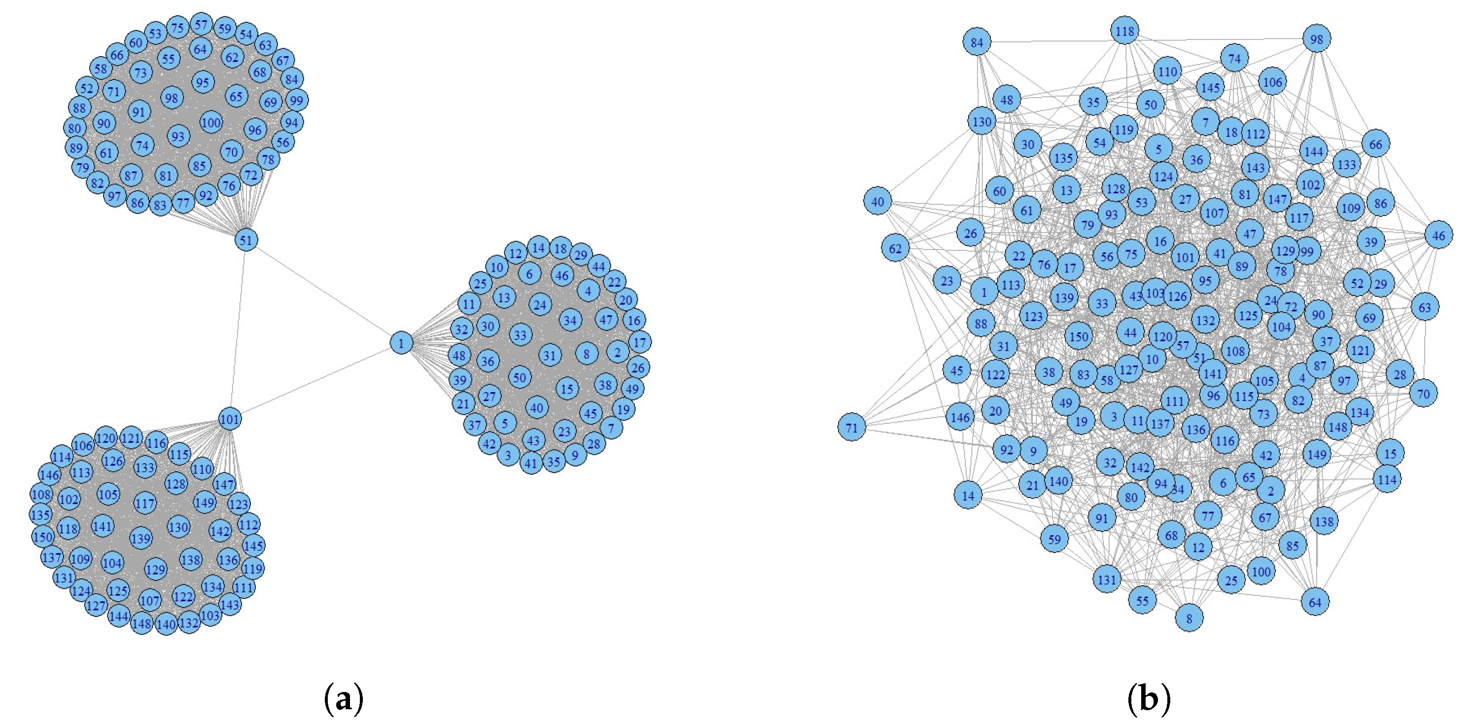
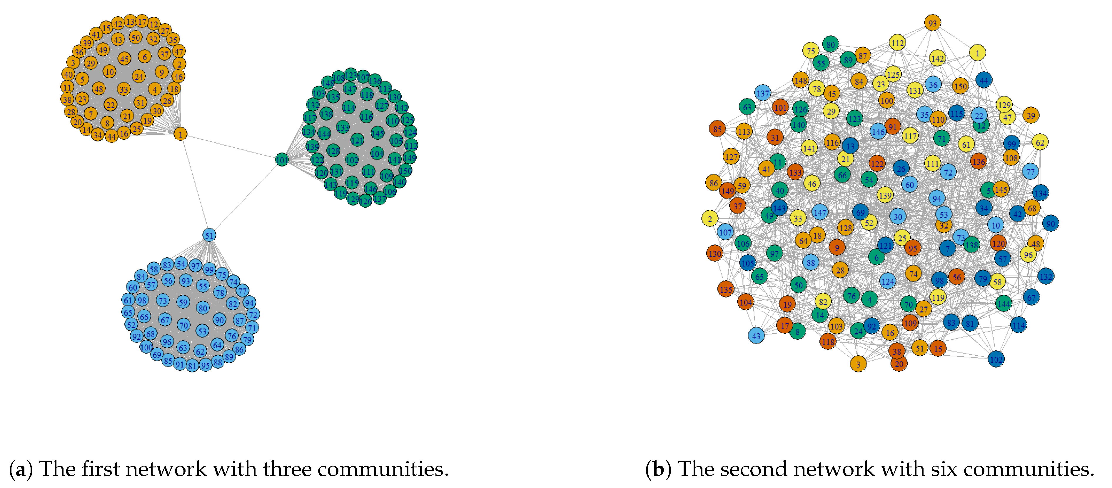
Figure 7.
Topological structure of the first and second company. (a) Network of the first company. (b) Network of the second company.
Figure 7.
Topological structure of the first and second company. (a) Network of the first company. (b) Network of the second company.
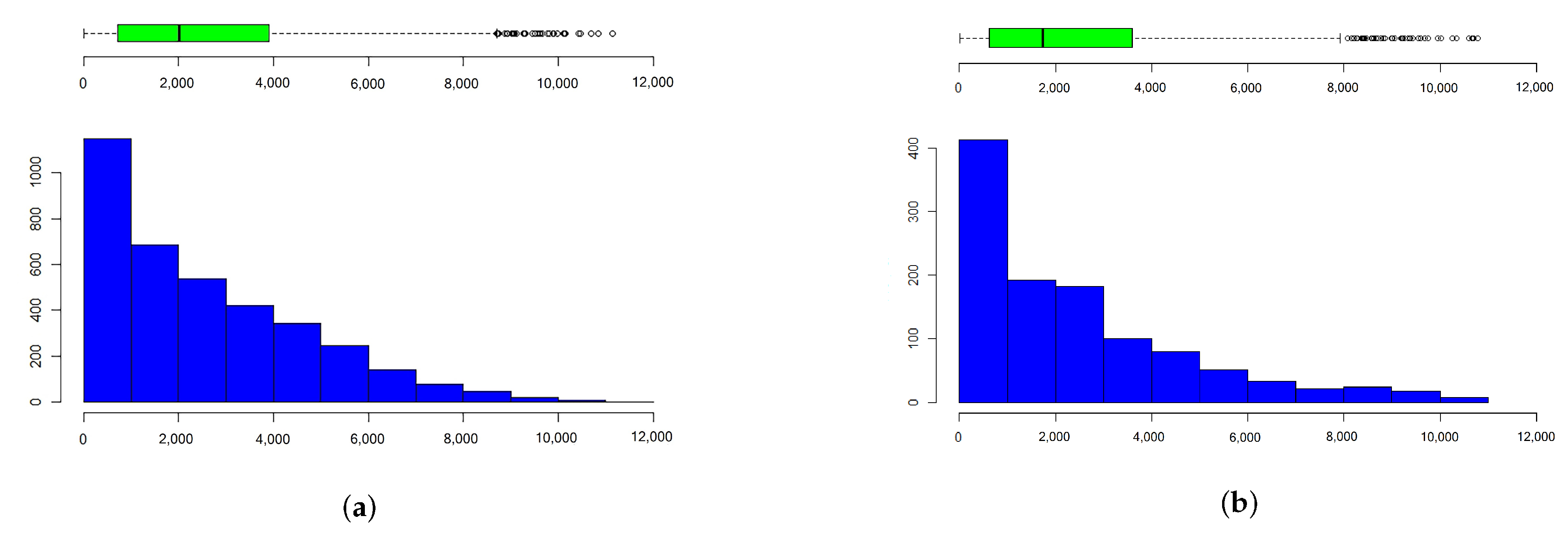
Figure 8.
Distribution of the number of communications for a 1-year contract follows a Poisson distribution with and according to a node-based model. (a) Distribution in the first network. (b) Distribution in the second network.
Figure 8.
Distribution of the number of communications for a 1-year contract follows a Poisson distribution with and according to a node-based model. (a) Distribution in the first network. (b) Distribution in the second network.
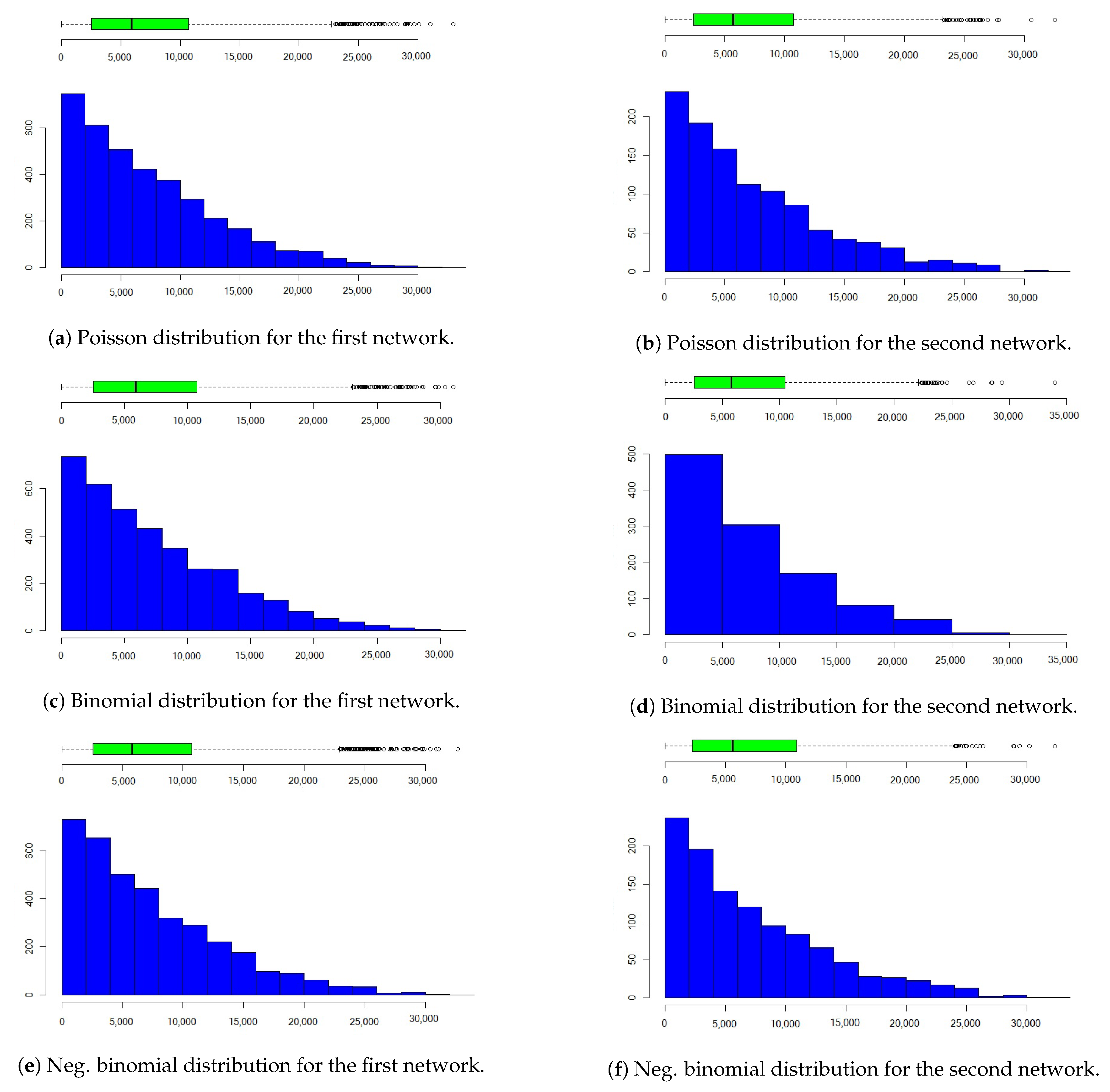
Figure 9.
Distributions of the number of communication for one year contract usiang a link-based model.
Figure 9.
Distributions of the number of communication for one year contract usiang a link-based model.
Figure 10.
Community detection of the weighted network for the first and the second company using the Louvain algorithm.
Figure 10.
Community detection of the weighted network for the first and the second company using the Louvain algorithm.
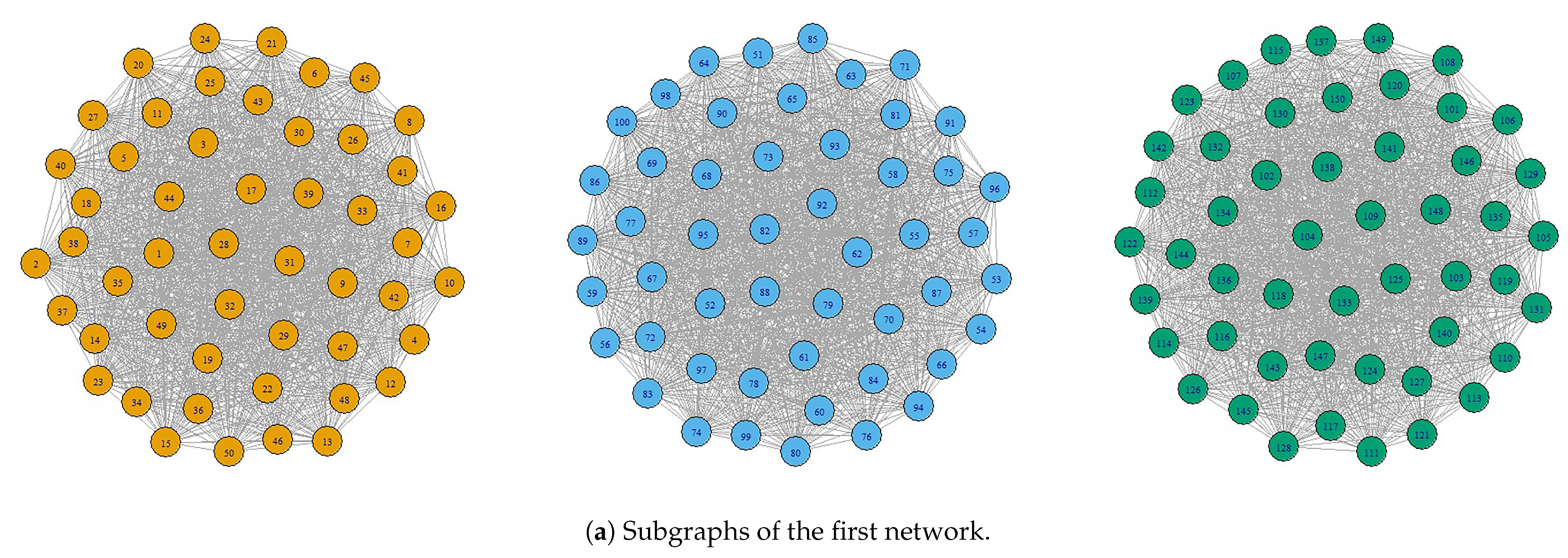
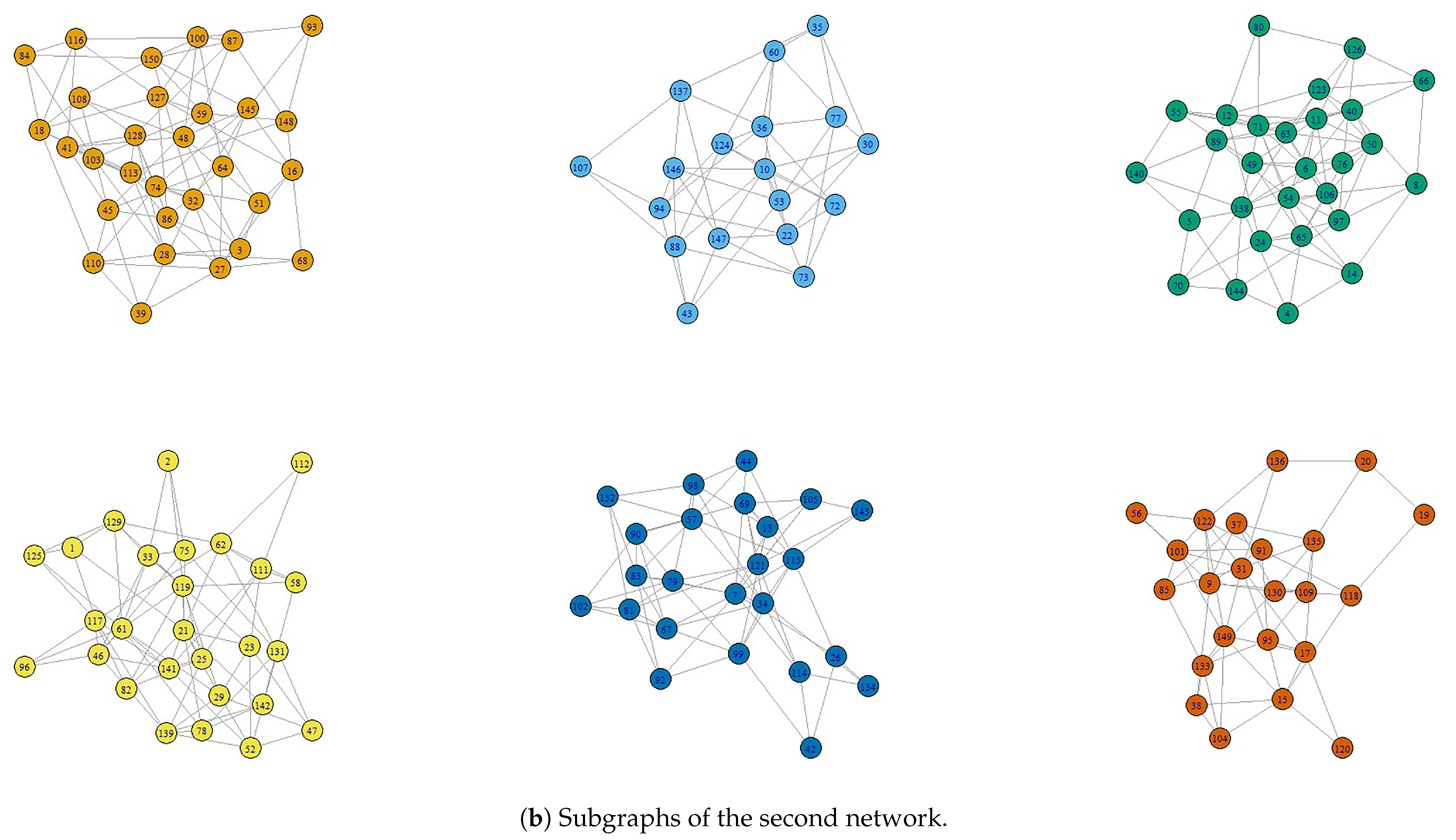
Figure 11.
Subgraphs or subnetworks of the first and second networks.
Figure 11.
Subgraphs or subnetworks of the first and second networks.
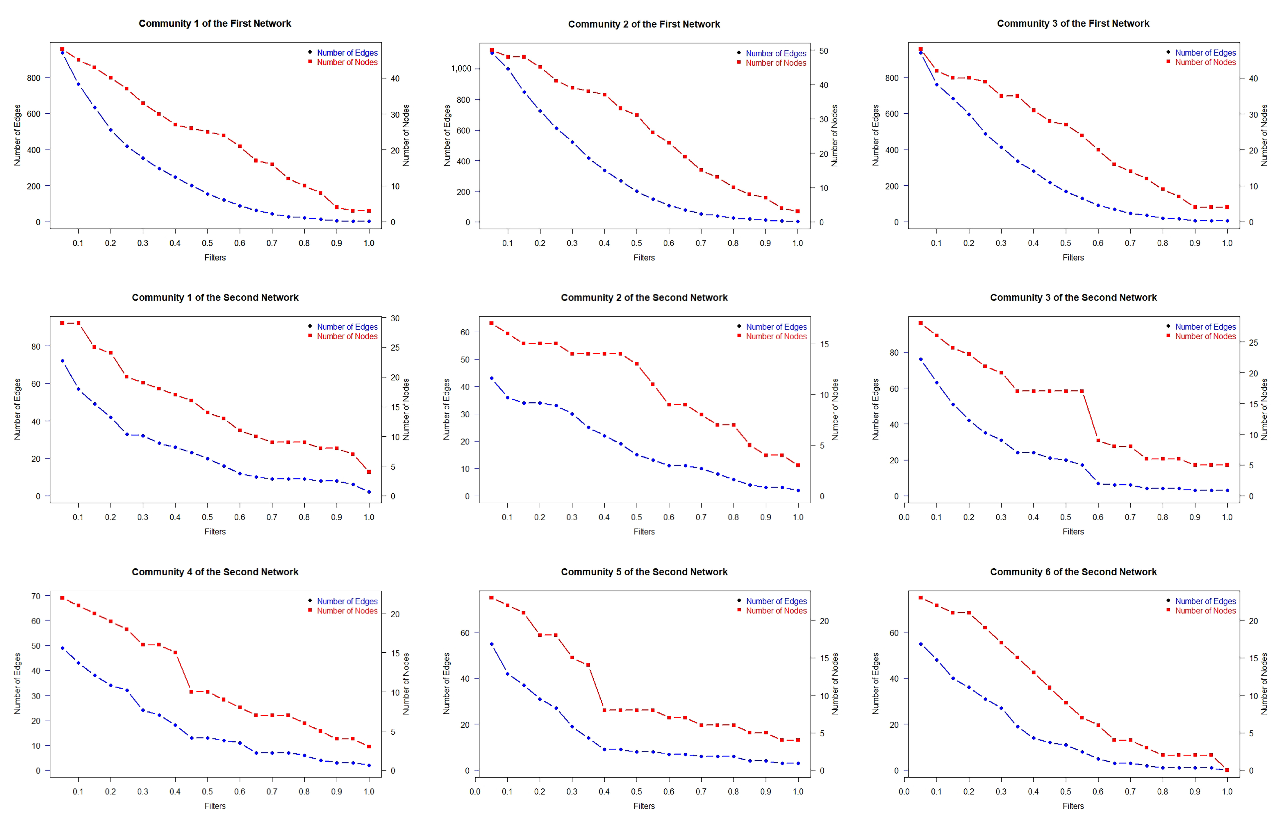
Figure 12.
Effect of filtering on the number of nodes and edges for each community in the first and second network.
Figure 12.
Effect of filtering on the number of nodes and edges for each community in the first and second network.
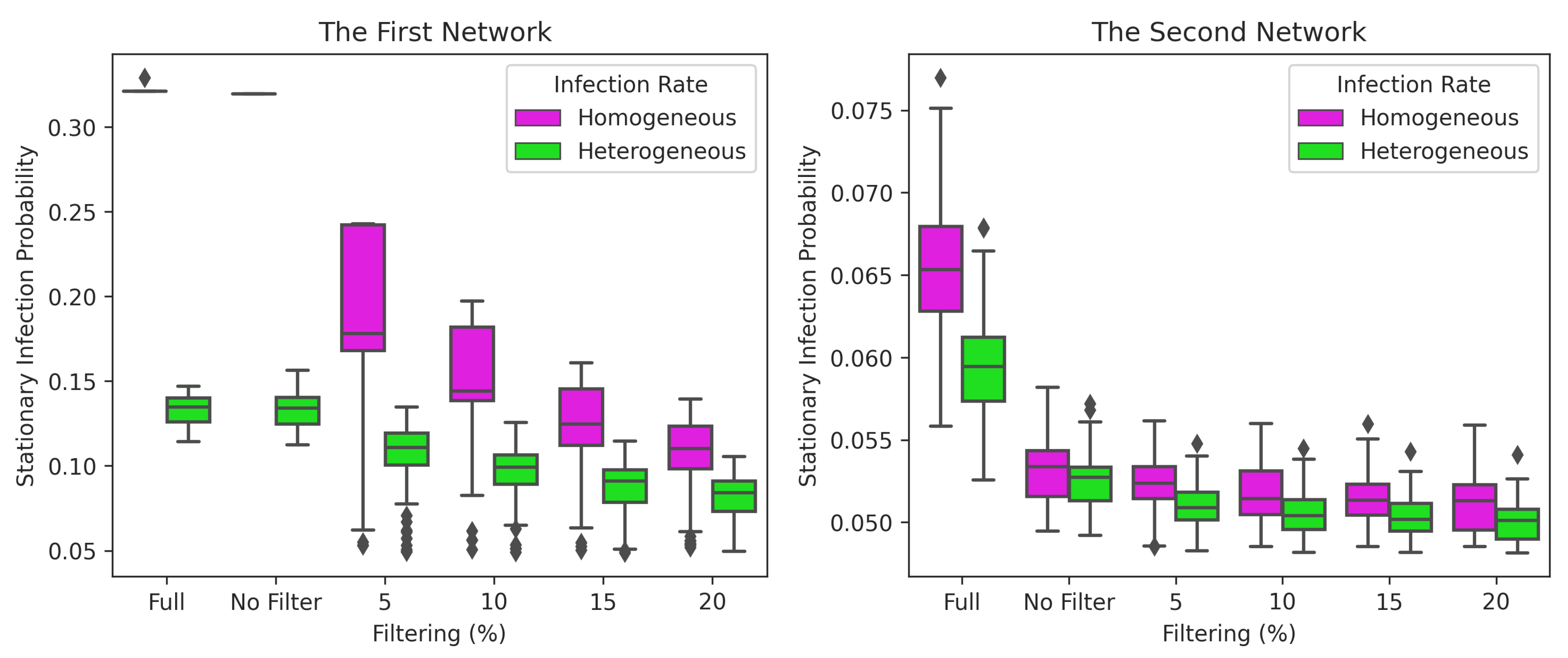
Figure 13.
Stationary infection probabilities of nodes based on filters and infection rates in the first and second network. There are two cases for homogeneous and heterogeneous infection rates: (1) without GMA (Full), and (2) with GMA (using filter 0% (No Filter), 5%, 10%, 15% and 20%).
Figure 13.
Stationary infection probabilities of nodes based on filters and infection rates in the first and second network. There are two cases for homogeneous and heterogeneous infection rates: (1) without GMA (Full), and (2) with GMA (using filter 0% (No Filter), 5%, 10%, 15% and 20%).
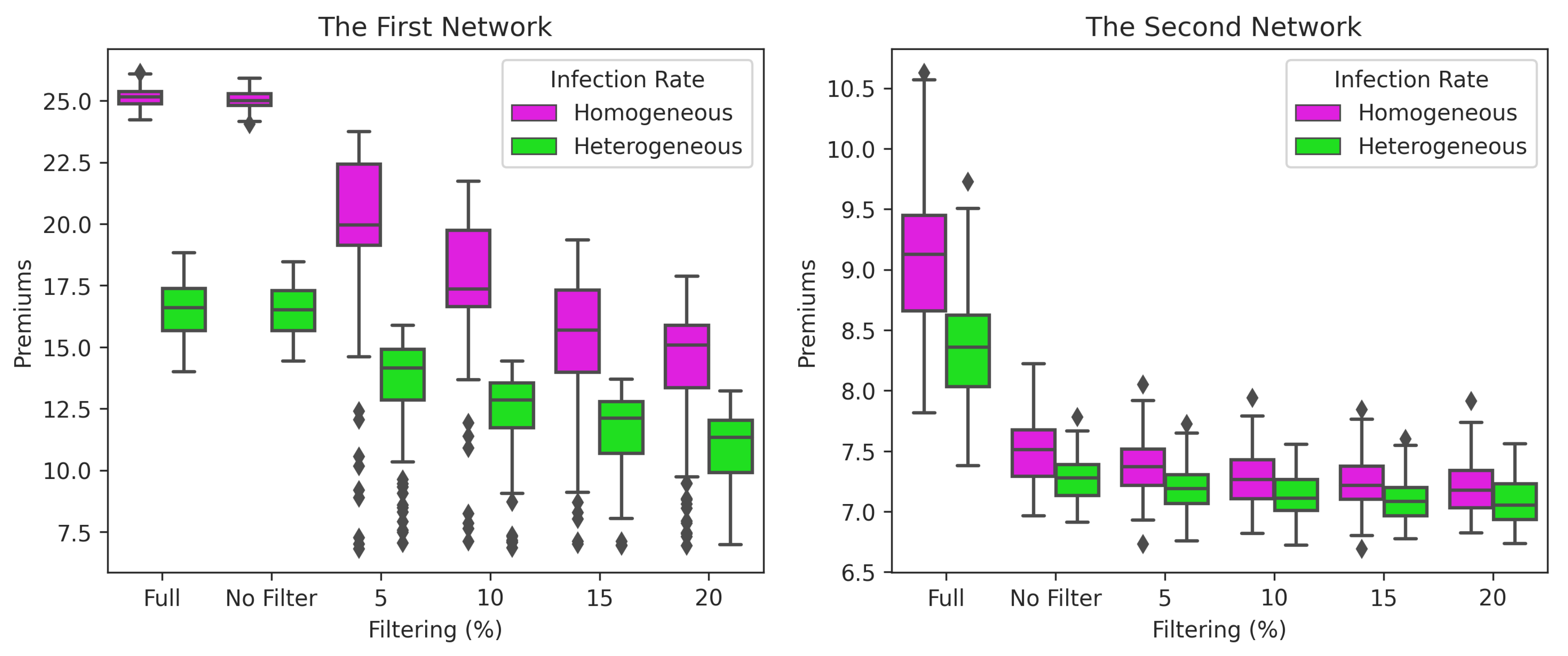
Figure 14.
Premiums of nodes based on filters and infection rates in the first and second network. There are two cases for homogeneous and heterogeneous infection rates: (1) without GMA (Full) and (2) with GMA (using filter 0% (No Filter), 5%, 10%, 15% and 20%).
Figure 14.
Premiums of nodes based on filters and infection rates in the first and second network. There are two cases for homogeneous and heterogeneous infection rates: (1) without GMA (Full) and (2) with GMA (using filter 0% (No Filter), 5%, 10%, 15% and 20%).
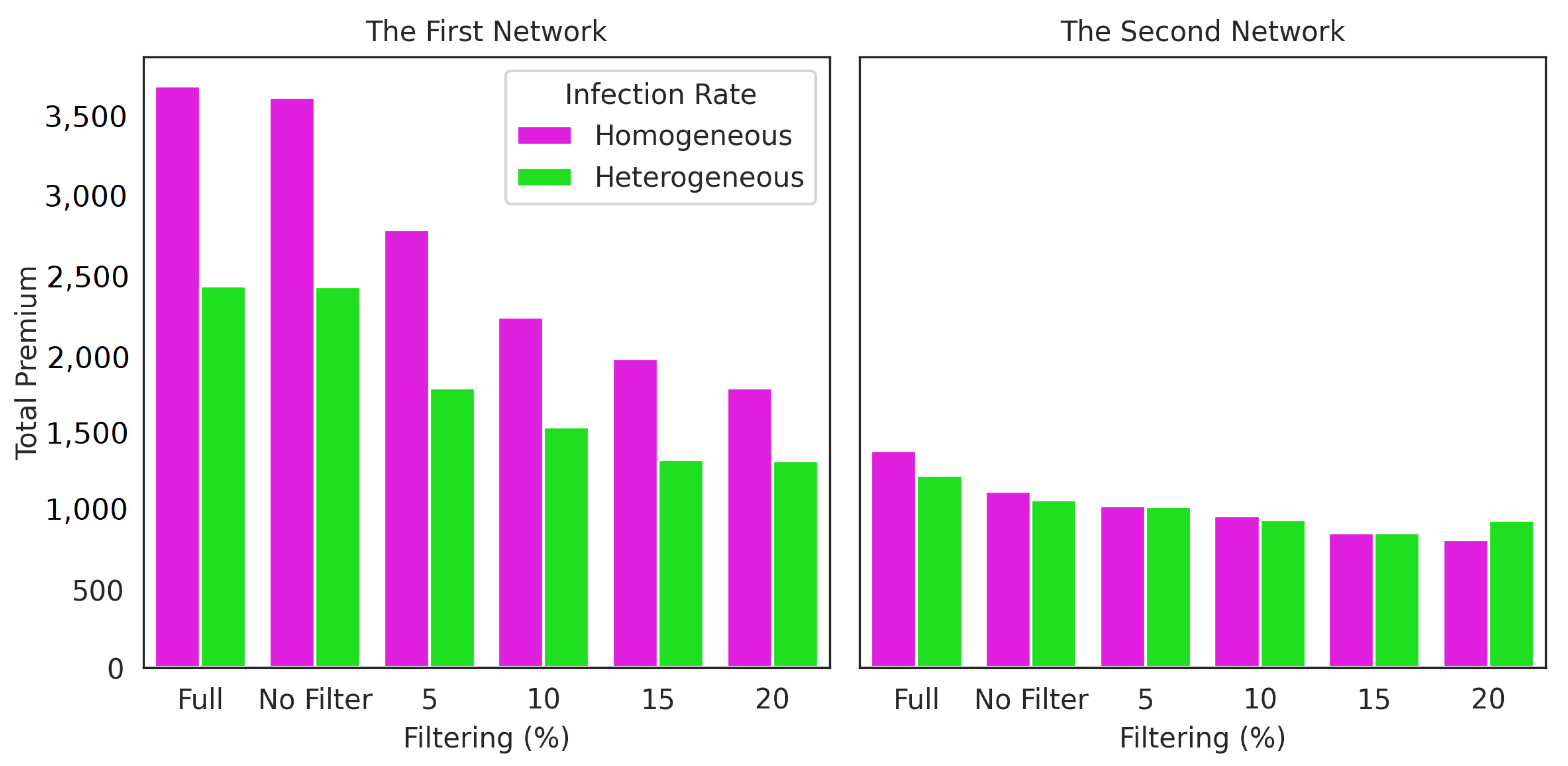
Figure 15.
Comparison of homogeneous total premium and heterogeneous total premium in the first and second network for two cases: (1) without GMA (Full) and (2) with GMA (using filter 0% (No Filter), 5%, 10%, 15% and 20%.
Figure 15.
Comparison of homogeneous total premium and heterogeneous total premium in the first and second network for two cases: (1) without GMA (Full) and (2) with GMA (using filter 0% (No Filter), 5%, 10%, 15% and 20%.
Figure 16.
Comparison of homogeneous total premium (
![Risks 09 00224 i004]()
), heterogeneous total premium (
![Risks 09 00224 i005]()
) and covered nodes (
![Risks 09 00224 i006]()
) in the first and second network for two cases: (1) without GMA (Full), and (2) with GMA (using filter 0% (No Filter), 5%, 10%, 15% and 20%.
Figure 17.
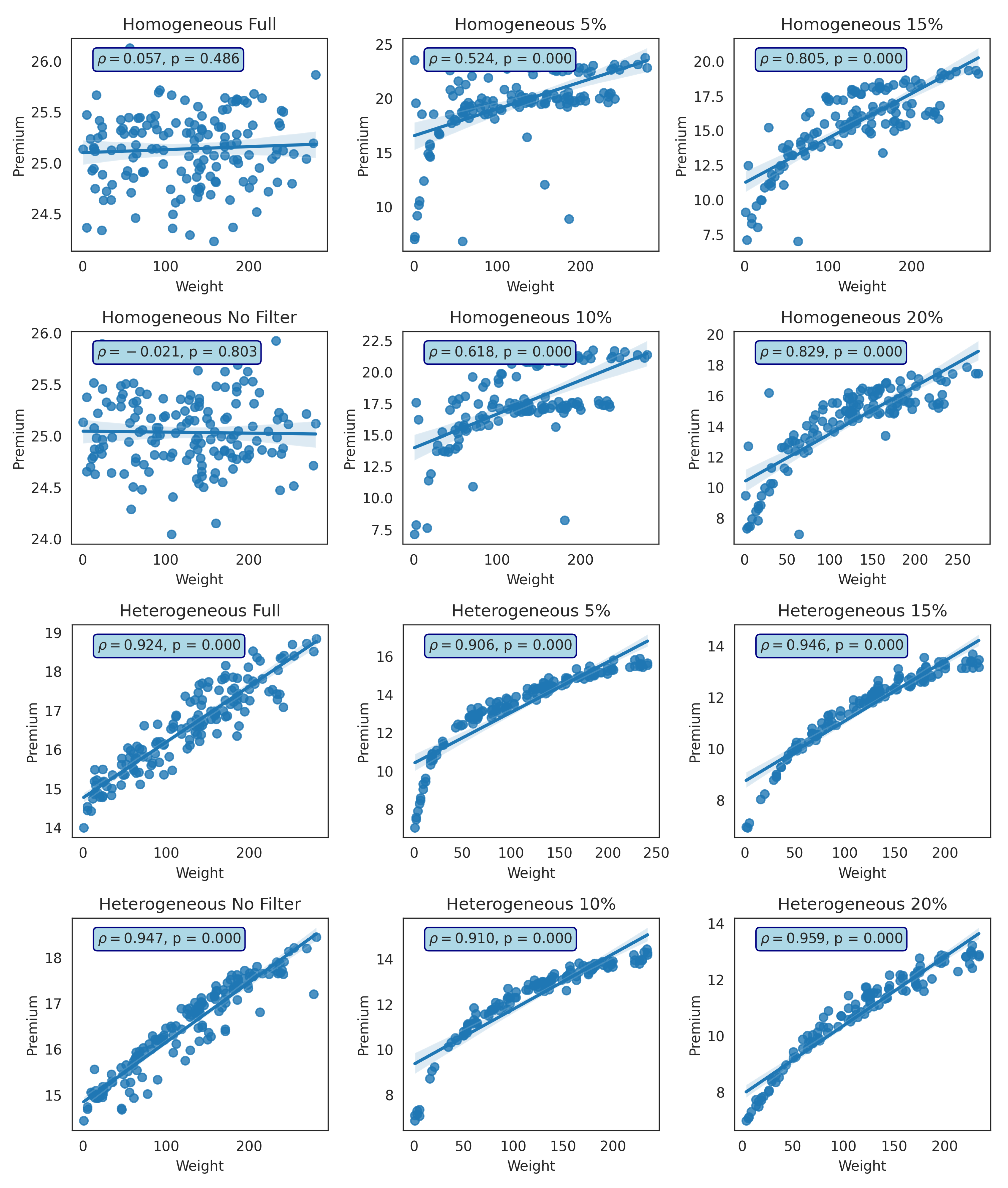
Relationship between the total weight of the neighbors and their premium (homogeneous and heterogeneous) for two cases: (1) without GMA (Full), and (2) with GMA (using filter 0% (No Filter), 5%, 10%, 15%, and 20% in the first network. is the Pearson correlation coefficient and p is the probability value.
Figure 18.
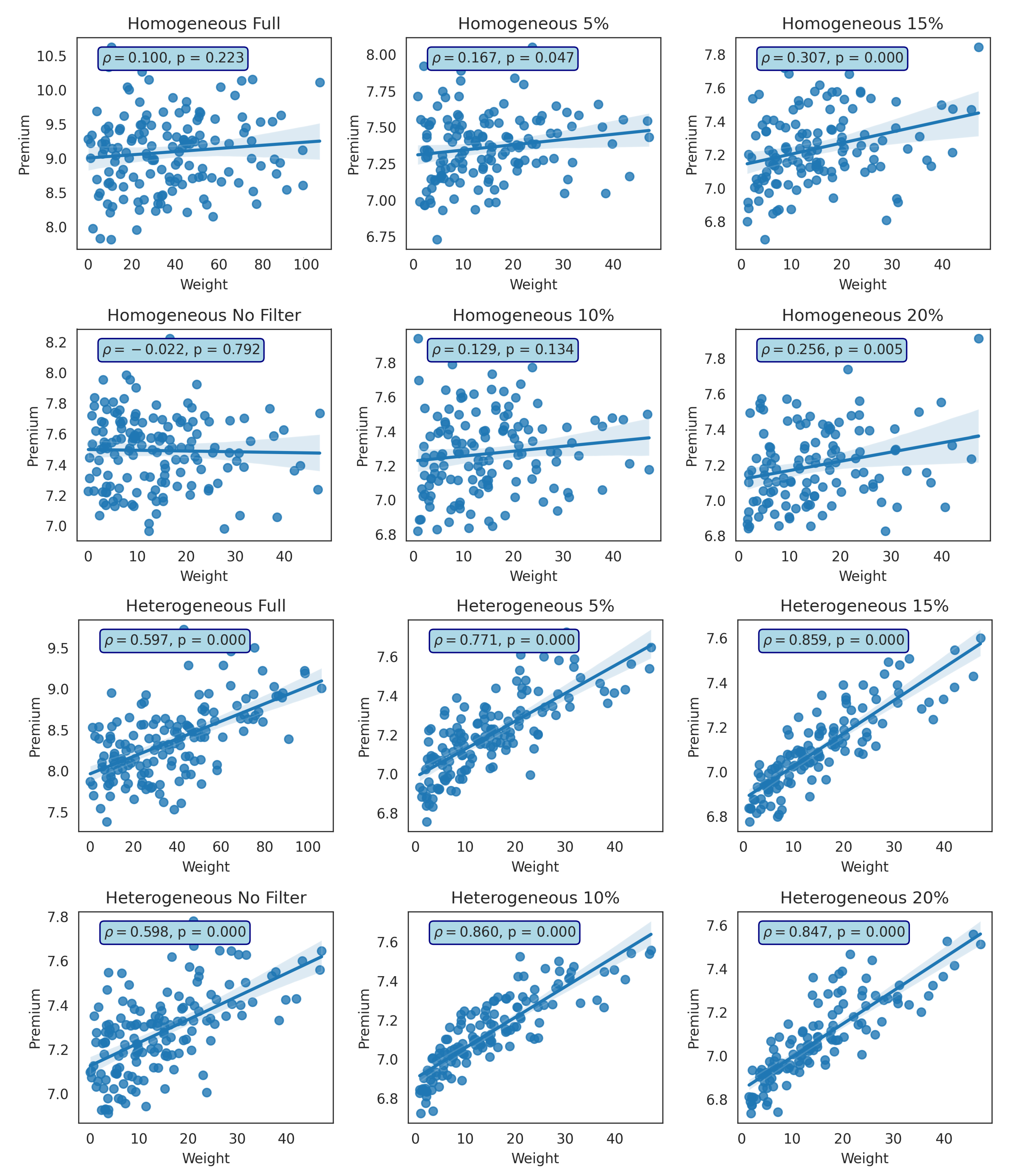
Relationship between the total weight of neighbors and their premium (homogeneous and heterogeneous) for two cases: (1) without GMA (Full), and (2) with GMA (using filter 0% (No Filter), 5%, 10%, 15%, and 20% in the second network. is the Pearson correlation coefficient and p is the probability value.
Table 1.
Comparison of the CIRM model. The-state-of-the-art of our proposed model, total loss, model input, and loss type.
Table 1.
Comparison of the CIRM model. The-state-of-the-art of our proposed model, total loss, model input, and loss type.
| Reference | Model | Total Loss | Input | Loss Type |
|---|
| Böhme and Kataria (2006) | Beta-binomial and one-factor latent model | Internal failure correlation | Cyberattack data | Loss function of stopping operation |
| Herath and Herath (2011) | Copula based model | Integrated copula-based simulation | The number of infected computers and their total loss. | First party damage due to a breach |
| Mukhopadhyay et al. (2013) | Collective risk model | Copula-aided Bayesian belief network (CBBN) | Twenty indicator variables (loss, system update, etc.) | General cybersecurity breaches |
| Eling and Wirfs (2015) | Extreme value theory | Value-at-Risk (VaR) dan Tail Value-at-Risk (TVaR) | Operational risk data of ICT assets | Internal and external errors of systems and humans |
| Fahrenwaldt et al. (2018) | Stochastic process (SIS model) | Marked point process and mean field aggregate | Network topology, infection and recovery rate, initial infections | Losses due to infections |
| Xu and Hua (2019) | Stochastic processes. Markov (-SIS model), non-Markov, and Copula | Monte Carlo simulation of infection and recovery process | Network topology, infection, recovery, and self-infection rate | Losses due to infection and losses due to service downtime |
| Hua and Xu (2020) | Stochastic process/non-Markov (Copula) | Monte Carlo simulation of infection and recovery process | The number of nodes and links, scale-free index, etc. | Losses due to service interruptions and losses related to computer repair costs |
| Antonio et al. (2021) (this paper) | Stochastic process/Markov (HG-SIS) | Monte Carlo simulation of infection and recovery process | Network topology, communication weight, and spreading parameters | Losses due to infection and losses due to service downtime |
Table 2.
Comparison of CIRM networks. The-state-of-the-art of our proposed network, risk selection, and communication effect.
Table 2.
Comparison of CIRM networks. The-state-of-the-art of our proposed network, risk selection, and communication effect.
Table 3.
Distribution of .
Table 3.
Distribution of .
| No. | Distribution | Parameter | |
|---|
| 1 | Poisson | | |
| 2 | Binomial | | |
| 3 | Negative Binomial | | |
Table 4.
Descriptive statistics for the weight of both networks according to the node-based model.
Table 4.
Descriptive statistics for the weight of both networks according to the node-based model.
| Network | n Links | Mean | SD | Median | Min | Max | 95th Perc. |
|---|
| First | 3678 | 2547.33 | 2162.83 | 2009.5 | 0 | 11,154 | 6787 |
| Second | 1126 | 2447.79 | 2352.23 | 1742 | 7 | 10,773 | 7635.8 |
Table 5.
Descriptive statistics for the weight of both networks created using a link-based model.
Table 5.
Descriptive statistics for the weight of both networks created using a link-based model.
| Desc. Stat. | Pois. 1st | Pois. 2nd | Bin. 1st | Bin. 2nd | Nbin. 1st | Nbin. 2nd |
|---|
| Mean | 7300.75 | 7303.28 | 7301.78 | 7299.8 | 7298.26 | 7299.78 |
| SD | 5904.14 | 6178.82 | 5883.68 | 5961.65 | 5974.05 | 6218.04 |
| Median | 5922.5 | 5727 | 5897.5 | 5799 | 5798.5 | 5622 |
| Min | 1 | 2 | 2 | 8 | 3 | 2 |
| Max | 32,931 | 32,539 | 31,020 | 33,972 | 32,629 | 32,290 |
| 95th perc. | 19,310.8 | 19,681 | 19,001.8 | 19,000 | 19,407.6 | 20,258 |
Table 6.
Threshlods for each community of the first and second networks.
Table 6.
Threshlods for each community of the first and second networks.
| Thresholds |
|---|
| Network | Community | tthet | tfhet | tvhet |
|---|
| First | 1 (orange) | 10,483.67 | 10,144 | 9928 |
| 2 (cyan) | 10,757.67 | 10,543.25 | 10,413.4 |
| 3 (green) | 10,082.33 | 10,055.25 | 9964.0 |
| Second | 1 (orange) | 8565.67 | 8520 | 8460.4 |
| 2 (cyan) | 9462 | 8916 | 8532.6 |
| 3 (green) | 9808.67 | 9263 | 8714 |
| 4 (yellow) | 9747.33 | 9294 | 8903 |
| 5 (blue) | 8453.33 | 8120.75 | 7786.4 |
| 6 (red) | 7192.67 | 6749 | 6473.6 |
Table 7.
Premiums and rates for the 15 selected nodes without GMA and with GMA with a 20% filter.
Table 7.
Premiums and rates for the 15 selected nodes without GMA and with GMA with a 20% filter.
| Without GMA (Full-Homogeneous) | With GMA with 20% Filter (Heterogeneous) |
|---|
| Node | Degree | Mean | Premium | Exposure | Rate | Degree | Mean | Premiums | Exposure | Rate |
|---|
| Panel A: The First Network |
| N2 | 49 | 65.94 | 25.334 | 53.932 | 0.47 | 4 | 17.632 | 6.827 | 9.123 | 0.748 |
| N9 | 49 | 63.78 | 24.619 | 134.328 | 0.183 | 29 | 18.73 | 7.164 | 114.069 | 0.063 |
| N12 | 49 | 67.12 | 25.617 | 141.949 | 0.18 | 29 | 19.616 | 7.636 | 120.692 | 0.063 |
| N33 | 49 | 64.62 | 24.494 | 63.816 | 0.384 | 11 | 17.523 | 6.766 | 26.368 | 0.257 |
| N50 | 49 | 66.32 | 25.105 | 79.67 | 0.315 | 20 | 17.408 | 6.752 | 52.929 | 0.128 |
| N51 | 51 | 64.42 | 23.937 | 251.816 | 0.095 | 41 | 25.759 | 9.889 | 235.85 | 0.042 |
| N78 | 49 | 64.94 | 24.8 | 239.146 | 0.104 | 40 | 25.915 | 9.971 | 225.796 | 0.044 |
| N79 | 49 | 66.8 | 25.49 | 215.663 | 0.118 | 40 | 24.258 | 9.283 | 203.809 | 0.046 |
| N89 | 49 | 65.16 | 24.296 | 77.454 | 0.314 | 12 | 17.256 | 6.614 | 30.648 | 0.216 |
| N100 | 49 | 67.08 | 26.56 | 60.916 | 0.436 | 4 | 17.375 | 6.7 | 8.855 | 0.757 |
| N140 | 49 | 67.12 | 25.449 | 157.99 | 0.161 | 34 | 20.699 | 7.938 | 144.656 | 0.055 |
| N142 | 49 | 67.68 | 25.934 | 87.413 | 0.297 | 24 | 17.558 | 6.795 | 64.526 | 0.105 |
| N143 | 49 | 65.66 | 24.2 | 68.076 | 0.355 | 14 | 17.445 | 6.863 | 33.304 | 0.206 |
| N144 | 49 | 66.54 | 25.75 | 83.511 | 0.308 | 23 | 17.528 | 6.765 | 59.724 | 0.113 |
| N145 | 49 | 67.7 | 25.698 | 184.6 | 0.139 | 36 | 22.655 | 8.697 | 173.27 | 0.05 |
| Panel B: The Second Network |
| N2 | 11 | 22.310 | 8.627 | 91.107 | 0.095 | 3 | 18.470 | 7.305 | 18.280 | 0.400 |
| N3 | 16 | 24.330 | 9.379 | 58.154 | 0.161 | 6 | 18.663 | 7.217 | 39.821 | 0.181 |
| N21 | 19 | 25.330 | 9.837 | 45.069 | 0.218 | 7 | 17.270 | 6.604 | 12.012 | 0.550 |
| N22 | 10 | 21.180 | 8.110 | 34.107 | 0.238 | 5 | 17.452 | 6.791 | 15.228 | 0.446 |
| N23 | 15 | 23.950 | 9.361 | 24.643 | 0.380 | 4 | 17.330 | 6.534 | 23.772 | 0.275 |
| N24 | 23 | 27.150 | 10.526 | 70.357 | 0.150 | 6 | 17.956 | 6.941 | 7.767 | 0.894 |
| N37 | 14 | 23.000 | 8.757 | 37.510 | 0.233 | 4 | 17.670 | 6.744 | 17.073 | 0.395 |
| N38 | 8 | 21.490 | 8.327 | 23.573 | 0.353 | 2 | 17.920 | 6.921 | 17.073 | 0.395 |
| N63 | 25 | 26.560 | 10.024 | 17.509 | 0.573 | 5 | 17.629 | 6.863 | 5.520 | 1.254 |
| N71 | 19 | 25.040 | 9.490 | 16.572 | 0.573 | 6 | 17.522 | 6.761 | 10.929 | 0.619 |
| N97 | 19 | 24.900 | 9.608 | 44.824 | 0.214 | 7 | 18.063 | 6.930 | 9.881 | 0.701 |
| N115 | 9 | 21.870 | 8.301 | 57.222 | 0.145 | 8 | 18.450 | 6.940 | 5.389 | 1.288 |
| N116 | 13 | 22.930 | 9.076 | 30.211 | 0.300 | 4 | 17.366 | 6.719 | 3.546 | 1.895 |
| N126 | 23 | 26.630 | 10.337 | 24.692 | 0.419 | 5 | 17.742 | 6.869 | 6.951 | 0.988 |
| N127 | 13 | 23.660 | 9.180 | 46.640 | 0.197 | 5 | 17.749 | 6.868 | 19.743 | 0.348 |

 ), heterogeneous total premium (
  ) and covered nodes (
  ) in the first and second network for two cases: (1) without GMA (Full), and (2) with GMA (using filter 0% (No Filter), 5%, 10%, 15% and 20%.
 ), heterogeneous total premium (
  ) and covered nodes (
  ) in the first and second network for two cases: (1) without GMA (Full), and (2) with GMA (using filter 0% (No Filter), 5%, 10%, 15% and 20%.
