Regional Government Revenue Forecasting: Risk Factors of Investment Financing

Abstract

Accurate revenue prediction is a key factor for the reliable determination of the investment part of entire regional and local budgets, particularly during economic downturns and fiscal uncertainty. An unexpected decline in revenue requires the reduction in capital expenditures and forces the regional government to find additional sources to close the budget gaps. Current studies indicate that budget forecasts often underpredict revenue and use the available information inefficiently. In this article, the authors examine chosen methods of forecasting regional government revenue. In addition to classical forecasting models based on time series and causal models, an original structural forecasting procedure was proposed, which is effective especially in case of data delay. The reliability of applied methods was assessed using data from the Polish area of Zachodniopomorskie over the period 2000–2018. The found evidence supported results that were obtained by many other researchers, which indicated that less comprehensive methods of forecasting can provide reasonably accurate estimates.

1. Introduction

Local and regional governments play a crucial role in both public finance and citizens’ welfare. To be able to carry out all their activities in a planned and organized manner, governments must have an accurate estimation of future revenue. The level of revenue in local government units depends, among other things, on the changes in the economic condition, the level of the inflow of external funds, the employment rate, the labour productivity, the level and quality of human capital, the functioning of the institutional environment and the effectiveness of the implemented economic and social policies (OECD 2009). This revenue is characterized by a certain degree of variability, which depends primarily on unexpected changes in economic activity, policy and administrative adjustments, or changing patterns of consumer demand (Freire and Garzon 2014). Additional uncertainty of future revenue of administrative units is created since the regional tax structure itself may be changed (Feenberg et al. 1989).

The potential overestimation of revenue may require unexpected constraints in expenditures, resulting in a reduction in investment activity and an increase in the volume of debt, and consequently may negatively determine the level of development of the community, the competitiveness of the local economy and local welfare (Galinski 2013; Krol 2013; Boukari and Veiga 2018). However under forecasting may lead to excessive tax levies and charges (Cirincione et al. 1999). Planning well for the delivery of government services and programs requires an accurate estimate of the revenue needed and costs related to carrying out all necessary activities (Willoughby and Guo 2008).

Anticipating the level of revenue is essential for both short- and medium-term planning of current and investment projects and for determining policy on the level and source of debt financing (Batóg 2011).

Without precise and accurate forecasts, governments will find it difficult to avoid budgetary shortfalls and to meet expenses, especially capital expenditures (Freire and Garzon 2014; Khan 2019).Physical capital, namely investment in infrastructure, has a determinant role in policies oriented towards stimulating the potential of regions, accelerating economic growth and reaching greater convergence (Quirino et al. 2014).

Proper revenue forecasting is also crucial for a sustainable fiscal program (Mikesell 2018) and it is a cornerstone of budget preparation especially in multiyear budgeting (Wildavsky 1986; Sun and Lynch 2008). Reliable estimates of revenue and expenditures can “provide an understanding of available funding; evaluate financial risk; assess the likelihood that services can be sustained; and identify the key variables that cause a change in the level of revenue” (National Advisory Council on State and Local Budgeting 2000). Especially during periods of fiscal decline, local governments pay increasing attention to revenue trends, and accurate revenue estimates can help manage budgetary equilibrium and increase citizens’ trust (Wong 1995; Voorhees 2004). For example during the recession that started in 2007, state tax revenue in the United States, as well as in many other countries, fell substantially and at the same time an increased demand for a range of services was observed and cuts in spending led to reductions in government employment. In the past states have drawn down their accumulated reserves, boosted revenue collection by increasing tax rates, eliminating tax exemptions or broadening the tax base. In some cases asset sales and delayed payments to suppliers were necessary due to automatic stabilizers such as debt limits or other fiscal rules (Jonas 2012). An important aspect of local government revenue forecasting is also the fact that this process is closely tied to public policy planning and implementation and is thus subject to considerable political pressure (Klay and Vonasek 2008; Penner 2008; Freire and Garzon 2014).

This paper is organized as follows. In the next part, chosen studies that focus on local and regional revenue forecasting and forecast errors are presented. The main objective and research hypothesis will be indicated in the third part, while the fourth section consists of discussion on some of the methodological approaches used in the forecasting of revenue of these governments, as well as their limitations. Data characteristics and received results and findings can be found in the fifth section of the study. The last part presents concluding remarks and potential directions for future research.

2. Literature Review

Four important themes are discussed in the local government revenue forecasting literature: revenue forecasting and the budgetary process, revenue forecasting techniques used, revenue forecasting accuracy and participation in the revenue forecasting process (Reddick 2008). According to Mikesell (2018), previous experience in revenue forecasting teaches, among others, the limits of econometrics, data problems, the need to understand tax structure, the influence of recessions and the reality of being wrong. Accurate budgetary forecasts rely not only on the knowledge of the regional economy and income structure but also on taxpayer behaviour, unexpected weather changes and international events (Sun 2008). An additional difficulty in accurately predicting local government revenue arises because variability, seasonality and sensitivity to different factors can differ for different types of revenue (Williams and Kavanagh 2016). Galinski (2013) conducted an extensive study to characterise the disparities between planned and executed local government revenue and expenditure in Poland between 2001 and 2011. He distinguished two sub-periods, i.e., the years 2001–2008, when underestimation was observed due to incorrectly predicted general subsidies, and 2009–2011, when revenue was overestimated, which resulted from excessively optimistic forecasts of their own revenue. Forecast accuracy was measured using mean absolute percentage error (MAPE) for the whole research period and was equal to 3.90% for total revenue, 4.53% for total expenditure and 20.59% in the case of capital expenditure. The latter overestimation caused severe cuts in public investment to be made by regional and local governments. The level of income generated by local government units significantly depends on the level of economic activity. For example, Batóg (2009), using the author’s proposal of the economic situation barometer, verified the hypothesis on the relationship between the economic situation and the level of revenue of local government units in Poland for the example of Zachodniopomorskie voivodeship in 2000–2008. The results obtained confirmed the existence of such a relationship, which had a non-linear character and was particularly visible when the time series of revenue was delayed by one period. Gianakis and Frank (1993) applied seven forecasting techniques: regression, moving average, Holt technique, single exponential smoothing, Box–Jenkins technique, general adaptive filtering and Winters technique to predict the yields of the 13 sources and the five aggregates of St. Petersburg’s revenue in the state of Florida. The average MAPE ranged between 10.30% (Box–Jenkins) and 42.36% (Winters) for specific methods, while the best accuracy rankings characterised the moving average and general adaptive filtering. The study of Williams and Kavanagh (2016) examined forecasts of 55 monthly, quarterly and annual local government revenue data series from 18 localities dispersed over 14 states in the United States with populations ranging from four thousand to one point four million and found evidence that damped trend methods and simple exponential smoothing methods performed best with monthly and quarterly data, while with annual data, naïve methods outperformed other methods.

Much attention in the literature has been paid to the issue of errors in forecasts of local and regional government revenue. Auerbach (1995) distinguished between three types of errors in the prediction of government revenue policy, economic and technical (behavioural). Policy errors were mainly due to mistaken fiscal policy. The last type of error was also characterised by Williams and Calabrese (2016). Economic errors are caused by wrong forecasts of macroeconomic parameters used in the budget projections, while technical errors might occur because of unexpected behavioural responses or model misspecification. Some authors point out that observed errors can arise from errors in the data and economic shocks that cannot be predicted at the time the forecast was made (Xu et al. 2008; Claudio et al. 2020). Other factors causing the occurrence of inaccurate revenue forecasts of local government units include: too long forecasting horizons, uncertainty about the size of external financing, changes in legal regulations and, in the long term, changes in the investment attractiveness of the region and demographic and migration processes. Lee and Kwak (2020), using Korean local government data from 2002–2016, found also that revenue volatility had statistically significant and consistent effects on forecast errors. Another factor contributing to the occurrence of errors in revenue forecasts is a significant serial correlation, which is when an error in an overly optimistic or pessimistic direction one year, increases the same error direction in the following year (Penner 2008). The direction of forecast errors differs according to the level of government. Among local governments, most research indicates that revenue underestimation is persistent and substantial (Rubin et al. 1999). The opposite phenomenon was found, for instance, by Boukari and Veiga (2018) for 308 Portuguese municipalities during the period 1998–2015, where total revenue was underestimated on average by 56.73%. Both kinds of inaccuracy patterns—over and underestimation—are quite common, as evidenced by previous studies (see e.g., Chatagny 2015).

It is worth noting, however, that when forecasts are calculated over a horizon of one financial year, their errors may be reduced by adjusting the forecast values during the current financial year using intra-annual information (Asimakopoulos et al. 2019). The accuracy of the forecasts can be assessed in relatively diverse ways; among the proposals we found analysis of variance, the Kruskall–Wallis procedure or approach based on rational expectations (Feenberg et al. 1989). However, the most widely used measure for assessing forecast accuracy was the MAPE, which is also used in this study.

3. Research Objective and Hypothesis

The primary objective of this study is to verify the effectiveness of selected methods of revenue forecasting on a regional basis. Indicating the methods, or the method characterized by the lowest forecasting errors, will make it possible to minimize the risk of underestimating or overestimating future revenue and, as a consequence, will provide a basis for building regional and local government budgets that are less biased by the risk of revenue and expenditure imbalances. Two different approaches will be analysed comparatively. The first is based on direct forecasting of local government revenue and is based on time series models. Several trend models and exponential smoothing models will be considered in this case (Gardner 1985). The second approach is based on a model of the dependence of local government revenue on the regional gross product, with the value of the latter variable being determined by four different methods: based on trend models, using the exponential smoothing models, based on a dependency model in which the explanatory variable is the number of persons employed and using the author’s approach referred to as structural forecasting. The proposed procedures for estimating regional gross product make it possible to avoid a time lag of two years in Polish official statistics for information on this variable concerning the release of gross domestic product data for Poland. Individual variants of forecasts were assessed in terms of the value of generated ex-post errors, the values of which constituted the criterion for selecting the best prediction method. This study was conducted on the example of the Zachodniopomorskie voivodship located in north-western Poland based on data from the period 2000–2018. All calculations have been made using MS Excel and STATISTICA.

The research hypothesis verified in this paper is the statement that the method of structural forecasting is characterized by high accuracy of obtained forecasts, which is higher in comparison to models of dynamics and dependency, not only in the occurrence of strong structural changes (economic shocks) but also in the conditions of stable economic growth.

4. Methodology

Techniques used in government revenue forecasting include both qualitative or judgmental (expert, naïve) approaches and quantitative methods. The latter includes accounting-based approaches, trend analysis, time series methods (incremental), econometric modelling (causal models) and microsimulation modelling (Frank 1990; Rubin et al. 1999). Examples of other methods used include predictive models with optimization based on genetic algorithms (Xie and Xie 2009), Bayesian estimation using information about social, economic and spatial relationships between regions (Polasek et al. 2010) or the rolling forecast approach, which is less sensitive to outliers than an approach that relies on forecasts based on only the first origin (Cirincione et al. 1999).

The selection of specific forecasting methods depends on the type of seasonality and periodicity, as well as the kind of revenue. A greater tendency to use a model-based approach is evident when the share of income depending on economic conditions in total income is significant. In case of the revenue sources with a high degree of uncertainty, such as new revenue and grants or asset sales, some qualitative forecasting methods, including consensus or expert forecasting, are more effective (Freire and Garzon 2014). Researchers generally have found that although quantitative methods outperform judgmental approaches (see e.g., Reddick 2004), local governments rely mostly upon judgmental forecasting (Frank 1993), while regional governments tend to use more methodologically sophisticated techniques (Frank and Gianakis 1990). Causal models require more extensive information than other methods (Cirincione et al. 1999), while many results indicate that simple methods, including trend analysis, as well as a mix of methods, both quantitative and qualitative, provide better accuracy (Willoughby and Guo 2008). The most complex forecasting techniques require extensive training, sizeable amounts of budgetary and economic data and are costly (Forrester 1991). The situation when forecasters employ their expertise on particular taxes, spending categories, determinants of revenue or spending categories to adjust quantitative output before finalizing forecasts is quite common (Frank and Zhao 2009). The accuracy of forecasts can be improved by using, in addition to standard macroeconomic quantities such as income and population, so-called dirty indicators, for instance, the types of restaurants visited by the population and the number of houses for sale on the market by the owner, not through a realtor (McDonald 2015).

A different area of discussion conducted in the field of forecasting economic variables, including local government revenue, is the problem of the level of data aggregation, i.e., comparing the effectiveness of direct and indirect forecasts. Many authors indicate that the use of indirect forecasting allows forecasts with a higher level of accuracy to be obtained (Pavía-Miralles and Cabrer-Borrás 2007).

An example of this approach can be found in (Kholodilin et al. 2007), where gross domestic product (GDP) was predicted for 16 German Länder using panel models and taking into account spatial dependencies. However, a large number of studies provide arguments in favour of obtaining better prediction results in the case of determining forecasts for single objects. Noteworthy among these are the results presented in the works of Zellner and Tobias (2000), Marcellino et al. (2003) and Demers and Dupuis (2005), which forecast, respectively, the average GDP growth rate for 18 industrialized countries, revenue and prices in the euro area and regional GDP growth in Canada. In the latter work, the authors emphasize that the direct approach makes it possible to take into account in the forecasting process the variation in the response of individual components of GDP to economic shocks occurring as a result of the specificity of individual regions, which leads to a decrease in the variance of the prediction. This study will use two different approaches to regional income forecasting. The first one (I) uses time series models of revenue. The first group consists of trend models, namely (Pindyck and Rubinfeld 1998):

-

Linear

$$y_t={\delta }_0+{\delta }_{1}t+{\epsilon }_t,$$

(1)

-

Exponential

$$\ln y_t={\delta }_0+{\delta }_{1}t+{\epsilon }_t,$$

(2)

-

Logarithmic

$$y_t={\delta }_0+{\delta }_1\ln t+{\epsilon }_t,$$

(3)

-

Power

$$\ln y_t={\delta }_0+{\delta }_1\ln t+{\epsilon }_t.$$

(4)

The second group consists of exponential smoothing models (Yaffee and McGee 2000):

-

Brown

$$m_t=\alpha Y_t+\left(1-\alpha \right)m_{t-1},$$

(5)

-

Holt linear

$$\begin{array}{c}{m}_t=\alpha Y_t+\left(1-\alpha \right)\left(m_{t-1}+{\delta }_{1,t-1}\right)\\ {\delta }_{1t}=\beta \left(m_t-m_{t-1}\right)+\left(1-\beta \right){\delta }_{1,t-1},\end{array}$$

(6)

-

With the exponential trend

$$\begin{array}{c}{m}_t=\alpha Y_t+\left(1-\alpha \right)\left(m_{t-1}{\delta }_{t-1}\right)\\ {\delta }_t=\beta \frac{m_t}{m_{t-1}}+\left(1-\beta \right){\delta }_{t-1},\end{array}$$

(7)

-

With the dampened trend

$$\begin{array}{c}{m}_t=\alpha Y_t+\left(1-\alpha \right)\left(m_{t-1}+\phi {\delta }_{t-1}\right)\\ {\delta }_t=\beta \left(m_t-m_{t-1}\right)+\left(1-\beta \right)\phi {\delta }_{t-1}.\end{array}$$

(8)

The second approach (II) is indirect. It assumes that revenue depends on a reference variable, which is the regional gross product, and is based on a model of the relationship between these variables (Equation (9)).

$$R_t=f\left(Regional Gross Produc{t}_t,{\epsilon }_t\right),$$

(9)

where:

• $R_t$—regional government revenue in period t,
• ${\epsilon }_t$—error term.

Parameters of the model (9) were estimated using the ordinary least squares method (OLS). This model was the basis for calculating regional government revenue forecasts. A similar way of forecasting is presented in the work of Williams and Calabrese (2016). In addition, since 2007, the US Central Statistical Office FEDSTATS has been estimating GDP values for metropolitan and non-metropolitan areas using the Bureau of Economic Analysis (BEA) methodology based on the proportion of GDP and population income (BEA 2015). In this approach, two variants of calculating the regional gross product are distinguished. In the first one, referred to as structural forecasting, the proportion between this volume and the gross domestic product is used to determine the value of the regional gross product (Equation (10)).

$$RegionalGrossProduc{t}_t={\delta }_{t-1}·GD{P}_t,$$

(10)

where:

• ${\delta }_{t-1}$—share of regional gross product in GDP in period t − 1.

In the second variant, the dependence of this variable on the number of employees by actual place of work, excluding those working in firms with less than five employees, is used to calculate the level of gross regional product.

5. Results

In Poland the total revenue of local governments consists of own revenue, general subsidy and special purpose grants. The share of local governments in personal income tax (PIT) and corporate income tax (CIT) tax revenue plays an important role in shaping their own revenue. The verification of the performance of the different methods was carried out for the total revenue generated by all local governments (communes, counties and Marshall part) in the Zachodniopomorskie voivodship. The procedure for assessing the effectiveness of the methods consisted of determining the revenue forecasts for 2016–2018, based on data from 2000–2015. The MAPE of forecasts was then calculated for each forecast.

Table 1. Total revenue of local governments, regional gross product and employed persons in Zachodniopomorskie voivodship and gross domestic product in Poland in 2000–2018.

Year	Zachodniopomorskie Voivodship			Gross Domestic Product in Poland (Million PLN)
	Total Revenue of Local Governments (Million PLN)	Regional Gross Product (Million PLN)	Employed Persons
2000	3409	32,867	-	748,483
2001	3730	33,686	-	781,548
2002	3664	34,473	-	812,214
2003	3596	34,774	299,439	847,152
2004	4111	37,410	302,765	933,091
2005	4662	39,864	308,422	990,530
2006	5188	42,730	317,304	1,069,431
2007	5864	46,626	326,915	1,187,508
2008	6459	51,087	334,061	1,285,571
2009	6566	53,093	322,006	1,372,025
2010	7191	55,453	329,610	1,446,844
2011	7666	58,857	326,577	1,565,251
2012	8222	61,004	324,394	1,623,442
2013	8509	61,521	329,362	1,646,724
2014	8854	64,291	332,199	1,711,244
2015	9177	68,008	333,903	1,801,112
2016	9900	69,559	343,202	1,863,487
2017	10,515	73,714	358,583	1,989,835
2018	11,327	78,252	364,110	2,121,555

Source: Statistics Poland, Local Data Bank.

presents data on the total revenue of local governments and the variables used in the different forecasting approaches and variants.

A noticeable decline in revenue occurred during the economic slowdown in 2002–2003, while the most recent global crisis resulted in only a significantly lower growth rate of this variable in 2009.

The forecasts and forecast errors obtained in the two approaches are presented below.

• Direct forecasts of revenue—time series models

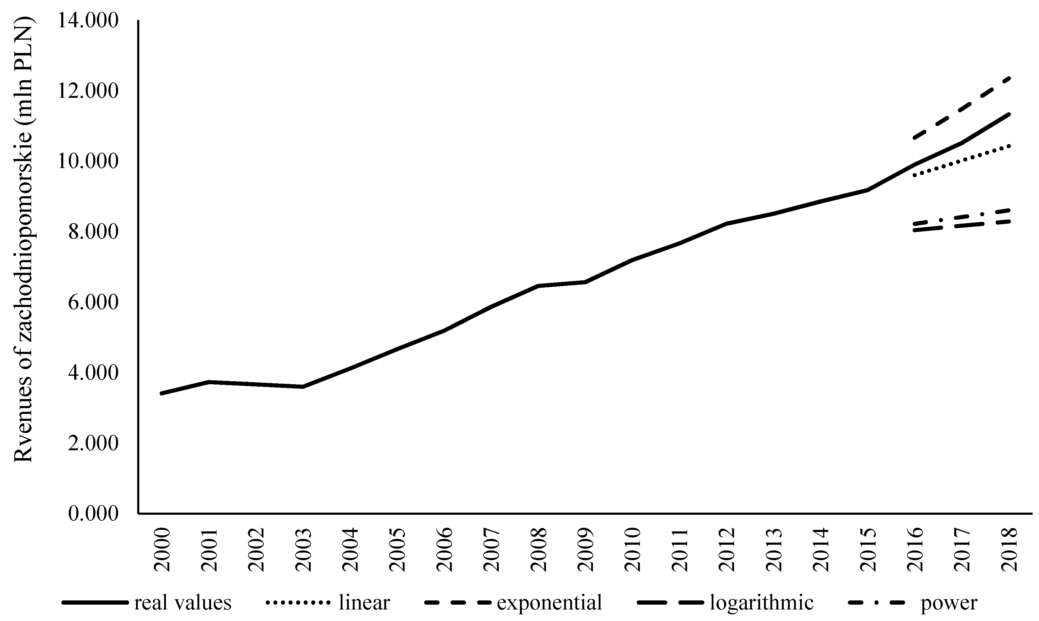
As a part of the first approach, revenue forecasts were obtained using four trend models (see

Table 2. Real values, forecasts, relative errors and MAPE’s for revenue of Zachodniopomorskie voivodeship in 2016–2018 (trend models, million PLN).

Year	Real Value	Forecasts				Relative Errors (%)
		Linear	Exponential	Logarithmic	Power	Linear	Exponential	Logarithmic	Power
2016	9900	9599.7	10,664.4	8040.9	8218.9	3.04	7.72	18.78	16.98
2017	10,515	10,012.8	11,474.6	8167.8	8413.8	4.77	9.13	22.32	19.98
2018	11,327	10,425.8	12,346.4	8288.2	8603.0	7.95	9.00	26.83	24.05
					MAPE	5.25	8.62	22.64	20.34
					MAE	567.82	914.57	2414.93	2168.67
					RMSE	620.18	921.06	2462.89	2210.53

and Figure 1).

The lowest MAPE value was found for forecasts based on linear trend. The quality of forecasts for exponential trend was slightly worse and the other two models generated very high error values, which definitely underestimated the revenue.

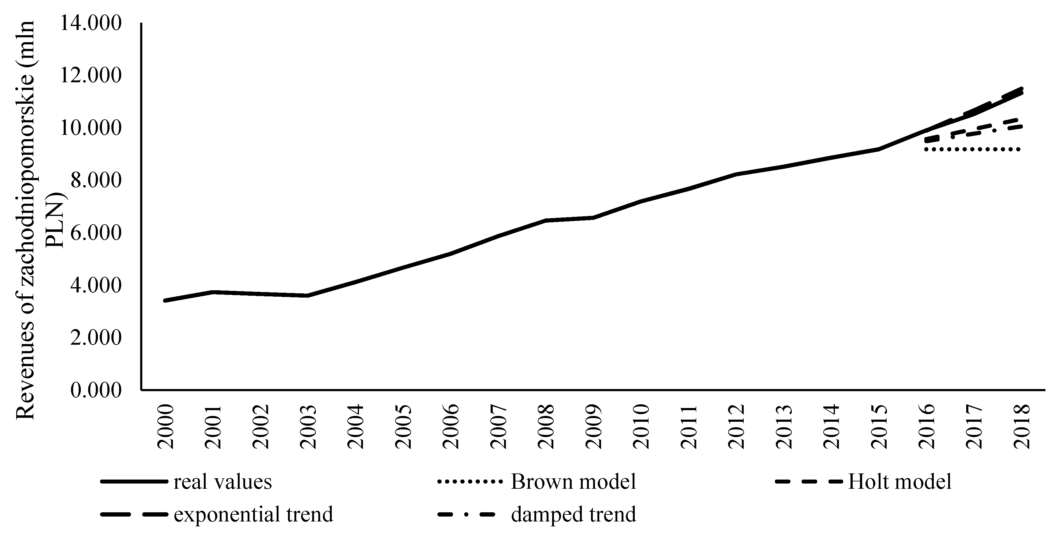
In the next step of the direct approach, forecasts were calculated based on four exponential smoothing models (see

Table 3. Real values, forecasts, relative errors and MAPE’s for revenue of Zachodniopomorskie voivodeship in 2016–2018 (exponential smoothing models, million PLN).

Year	Real Values	Forecast				Relative Errors (%)
		Brown Model	Holt Model	Exponential Trend	Damped Trend	Brown Model	Holt Model	Exponential Trend	Dampened Trend
2016	9900.3	9176.5	9563.3	9889.8	9483.5	7.31	3.40	0.11	4.21
2017	10,514.8	9176.5	9948.7	10,657.8	9773.9	12.73	5.38	1.36	7.05
2018	11,326.6	9176.5	10,334.2	11,485.4	10,049.0	18.98	8.76	1.40	11.28
					MAPE	13.01	5.85	0.96	7.51
					MAE	1404.12	631.85	104.11	811.78
					RMSE	1520.78	687.74	123.52	886.00

and Figure 2).

In the case of the Holt model we observed an error level close to the error values obtained for the linear trend. However, a very low MAPE value was obtained for the exponential smoothing model with an exponential trend.

II

Indirect forecasts of revenue

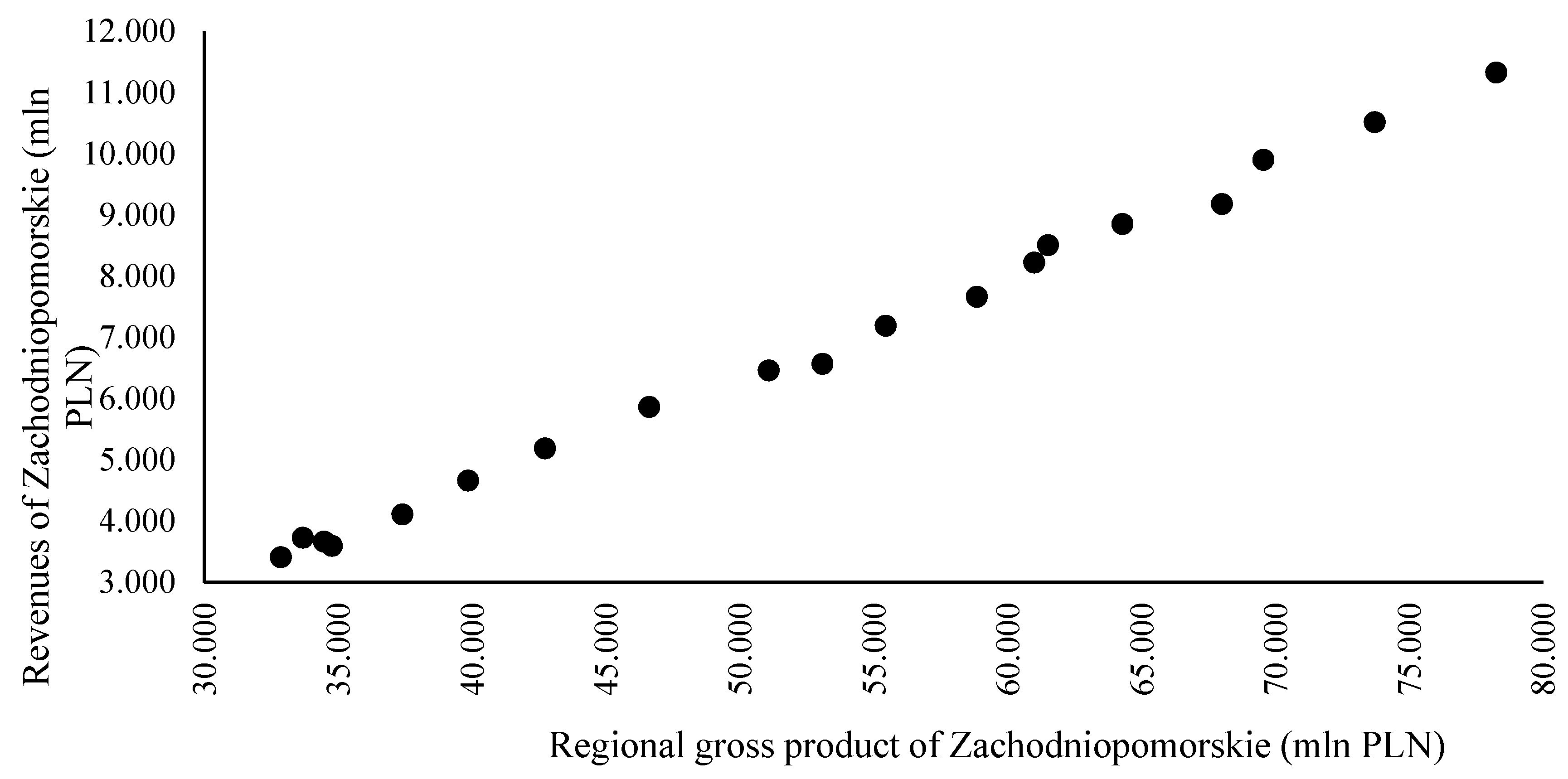
Figure 3 presents the relationship between revenue and regional gross product of Zachodniopomorskie voivodeship.

The shape of the scatter of points representing individual observations allows the formulation of a conclusion on the occurrence of a strong positive correlation of these variables and a hypothesis on the linearity of this relationship. The results of the OLS estimation of parameters of the model describing this relationship are presented in

Table 4. Results of estimation of the model for revenue (dependent variable) and regional gross product (independent variable) of Zachodniopomorskie (model 9).

	Coefficient	Standard Error	t Statistics	p-Value
Constant	−2107.974	153.400	−13.742	0.001
Regional gross product of Zachodniopomorskie	0.168	0.003	54.758	0.001

R² = 0.995; Standard error of estimation = 144.9; F(14,1) = 2998.39, p = 0.001.

.

We can see that model 9 is characterized by a high degree of fitting to the real data and significant structural parameters. It is worth noting that the presented relationship is not disturbed by periods of economic slowdown, which occurred in 2001–2003 and 2009. The obtained results indicate that with an increase in the regional gross product of the voivodeship by one million PLN, the total revenue of local governments increased in the analysed period on average by 168 thousand PLN.

Variant A—forecast of the regional gross product based on the number of employed persons.

In this variant, the value of the predictor appearing in model 9 in the form of the regional gross product is calculated based on the model of the relationship between this product and employed persons. The results of OLS estimation of parameters of this model obtained, based on data from 2000–2015, are presented in

Table 5. Results of estimation of the model for the regional gross product (dependent variable) and employed persons (independent variable) in Zachodniopomorskie (model 10).

	Coefficient	Standard Error	t Statistics	p-Value
Constant	−204,562.856	46,288.705	−4.419	0.001
Employed persons in Zachodniopomorskie	0.796	0.144	5.544	0.001

R² = 0.736; Standard error of estimation = 5815.7; F(12,1) = 30.74, p = 0.001.

.

Model 10 is not of such high quality as model 9, nevertheless, its degree of fit to the empirical data is satisfactory and its structural parameters are statistically significant. Using model 10, in which the values of the employed persons in 2016–2018 were determined as forecasts based on the linear trend of this variable, forecasts of gross regional product and their relative ex-post errors were calculated.

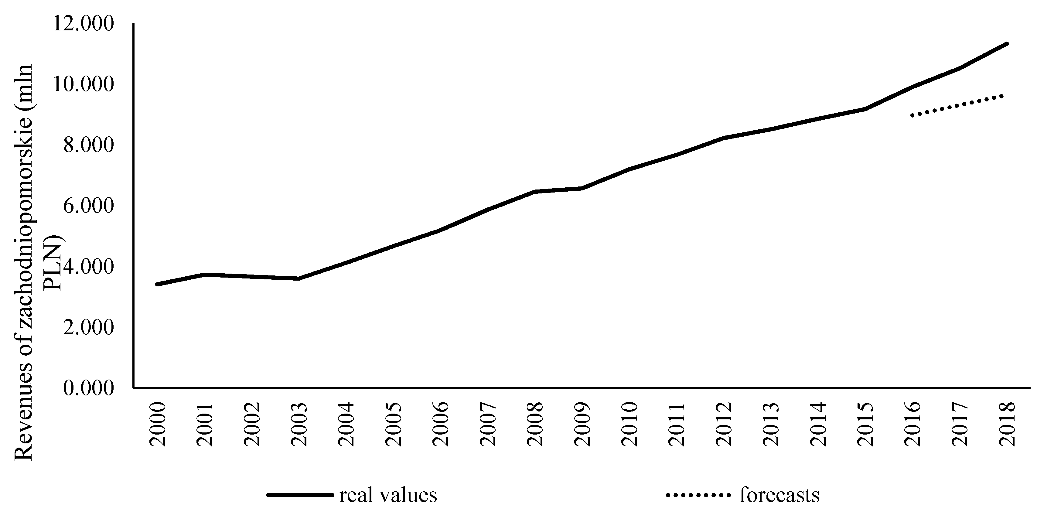
Based on forecasts of the regional gross product of Zachodniopomorskie voivodship presented in

Table 6. Forecasts of employed persons (linear trend) and regional gross product of Zachodniopomorskie voivodship (based on model 10).

Year	Forecasts of Employed Persons in Zachodniopomorskie	Forecasts of Regional Gross Product of Zachodniopomorskie (Million PLN)	Relative Error of Forecasts (%)
2016	339,529.65	65,801.47	5.40
2017	342,023.37	67,787.19	8.04
2018	344,517.09	69,772.92	10.84
		MAPE	8.09
		MAE	6054.47
		RMSE	6354.55

, forecasts of revenue of Zachodniopomorskie voivodship were calculated using model 9. Their values are presented in

Table 7. Forecasts of revenue and their errors for Zachodniopomorskie (based on model 9 and forecasts of regional gross product based on model 10).

Year	Forecasts of Revenue of Zachodniopomorskie (Million PLN)	Relative Error of Forecasts of Revenue of Zachodniopomorskie (%)
2016	8969.49	9.40
2017	9303.78	11.52
2018	9638.07	14.91
	MAPE	11.94
	MAE	1276.80
	RMSE	1314.56

and Figure 4.

We can see that the accuracy of revenue forecasts for the Zachodniopomorskie obtained, based on the model of the relationship between gross product and the number of employees, is not very high.

Variant B—the forecast of the regional gross product obtained from the proportion of this variable to the GDP of Poland.

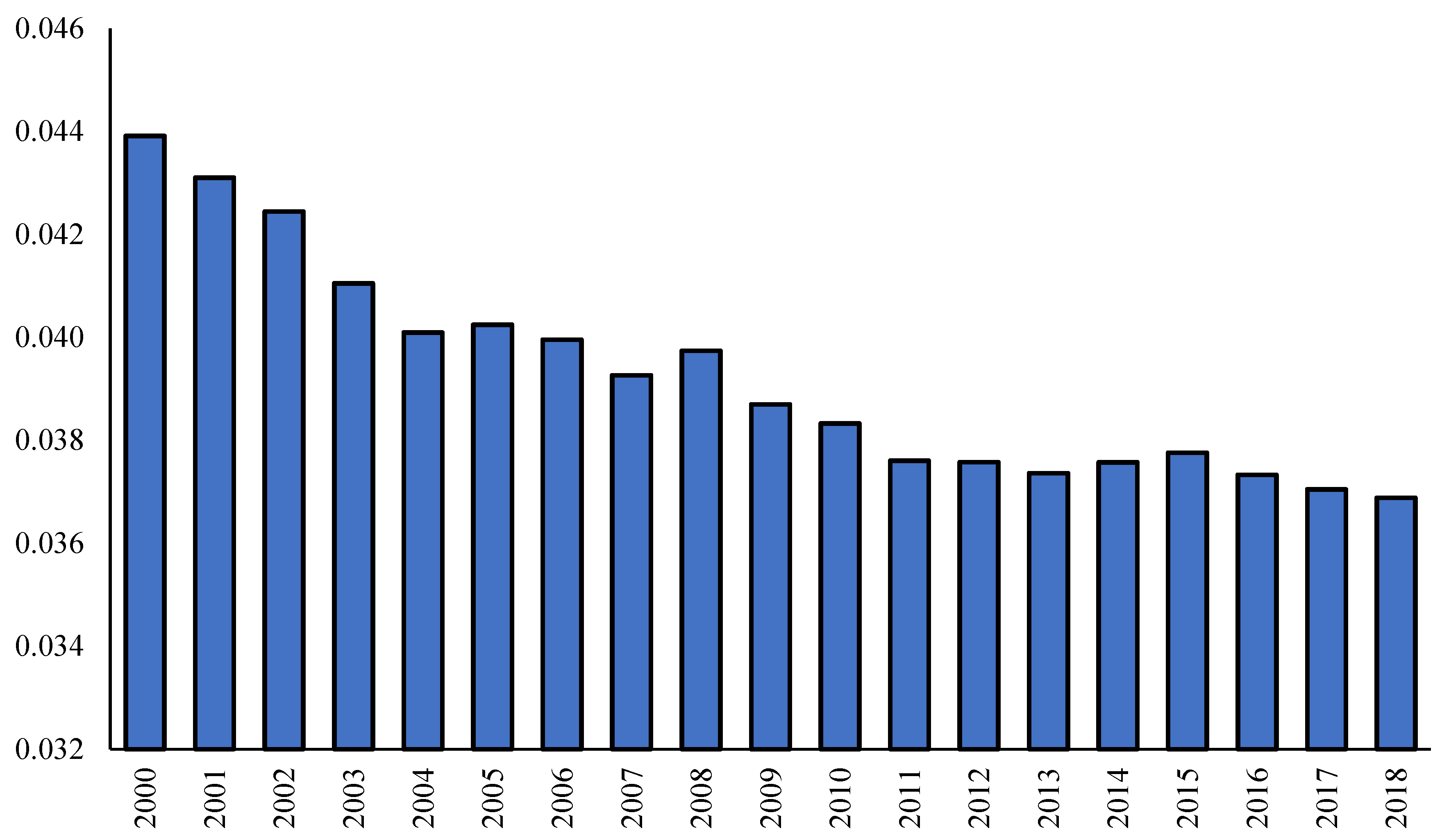
Figure 5 presents the dynamic of the share of the regional gross product of Zachodniopomorskie voivodship in the GDP of Poland in 2000–2018.

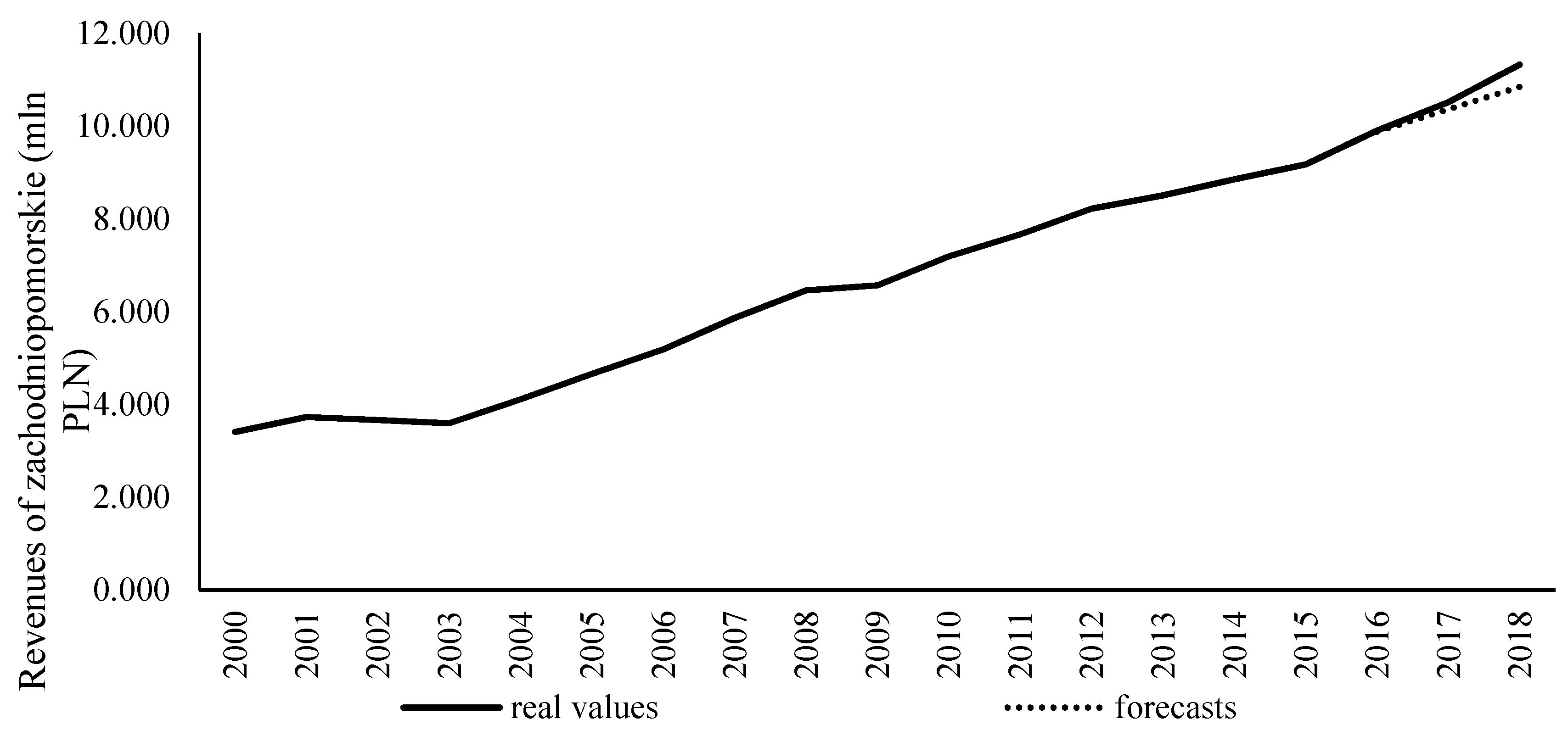
This proportion decreased quite rapidly in the early years, and since 2011 has remained at a similar level: 3.7–3.8%. Revenue forecasts for the Zachodniopomorskie voivodeship for 2016–2018 were calculated using the 2015 proportion and forecasts of the gross domestic product derived from a linear trend model (see

Table 8. Forecasts of gross product, revenue and their relative errors for Zachodniopomorskie (based on model 9, forecasts of GDP—linear trend and structural forecasts of the regional gross product of Zachodniopomorskie).

Year	Structural Forecasts of Gross Product of Zachodniopomorskie (Million PLN)	Forecasts of Revenue of Zachodniopomorskie (Million PLN)	Relative Error of Forecasts of Revenue of Zachodniopomorskie (%)
2016	71,206.24	9879.36	0.21
2017	74,080.04	10,363.16	1.44
2018	76,953.84	10,846.95	4.23
		MAPE	1.96
		MAE	217.43
		RMSE	290.69

and Figure 6).

Variant A and variant B apply the same multi-stage procedure. The consecutive steps in variant A are as follows: forecasting the employed persons in the region, forecasting the regional gross product and then forecasting the revenue of the region. In variant B we calculate successively as follows: the forecast of the gross domestic product, the forecast of the regional gross product and then we forecast the revenue of the region. A comparison of the MAPE values, determined for the two variants, clearly showed the advantage of forecasting revenue using the structural approach, which is less effective than the exponential smoothing model with the exponential trend only. Both methods, in terms of forecast accuracy, clearly dominated all the other methods proposed in the study carried out and, at the same time, both underestimated revenue.

6. Conclusions

During fiscal stress, local and regional governments are facing a decrease in revenue. In many cases if they do not properly plan their expenditure they are focused on how to cut investment to balance the current budget. One of the ways to reduce the risk of such a situation occurring are activities aimed at building an efficient revenue forecasting system, which requires not only identification of changes in the revenue structure and factors determining their level, but also selection of a reliable forecasting method. In a situation of rapid structural changes, both in the financial and real spheres of the economy, it is relatively difficult to make accurate forecasts based on classical prediction procedures. At the same time during those periods, the accuracy of revenue forecasts deteriorates (Mikesell 2018). It seems that in the process of formulating economic and fiscal policy, methods using structural proportions between the phenomena under study may then be applicable. An example of the application of this type of approach against the background of alternative regional revenue forecasting methods is presented in the study carried out. An additional advantage of directly relating revenue to the regional gross product is the ability to simulate the change in revenue with assumed changes in GDP and, consequently, to build scenarios for responding in advance to anticipated revenue shortfalls. Necessary reductions in expenditure, including capital expenditure, can then be carried out more smoothly and in certain situations can be avoided by providing the desired level of funding in advance. Reliable information on the projected change in revenue also makes it possible to determine the level of expenditure that does not result in the local government budget being out of balance and, above all, can provide a hedge against the risk of over indebtedness.

The forecasting results obtained based on the three approaches, time series models, dependency models and structural forecasting, allow us to state that the most effective methods of forecasting local government revenue are exponential smoothing with the exponential trend (MAPE = 0.96) and structural forecasting using the ratio of regional gross product to gross domestic product (MAPE = 1.96). Therefore, these results confirm the usability of less advanced methods in forecasting regional government revenue.

It should be remembered, however, that when significant structural change is occurring in the economy, expert knowledge should be used in addition to quantitative inference, and econometric forecasts should be supplemented with growth scenarios, especially over a long forecast horizon.

Calculated values of forecasts for the whole region (Zachodniopomorskie voivodeship) can be the basis for forecasts of revenue of its components, i.e., communes, counties and Marshall part. This can be performed, for example, by using the proportions of revenue between local government units or disaggregation procedures based on sets of associated variables such as, for example, the value of production, the gross value of fixed assets or the level of investment (Tokarski 2013; Ciołek 2017).

As part of further research carried out in the area of local government revenue forecasting, it is worth extending the research sample significantly, analysing not only Polish but also European local governments. A separate emphasis can be placed on the assessment of the impact of emerging economic crises on the accuracy of revenue forecasts. The spectrum of forecasting methods used could also be broadened.