Global Stock Selection with Hidden Markov Model

Abstract
:1. Introduction
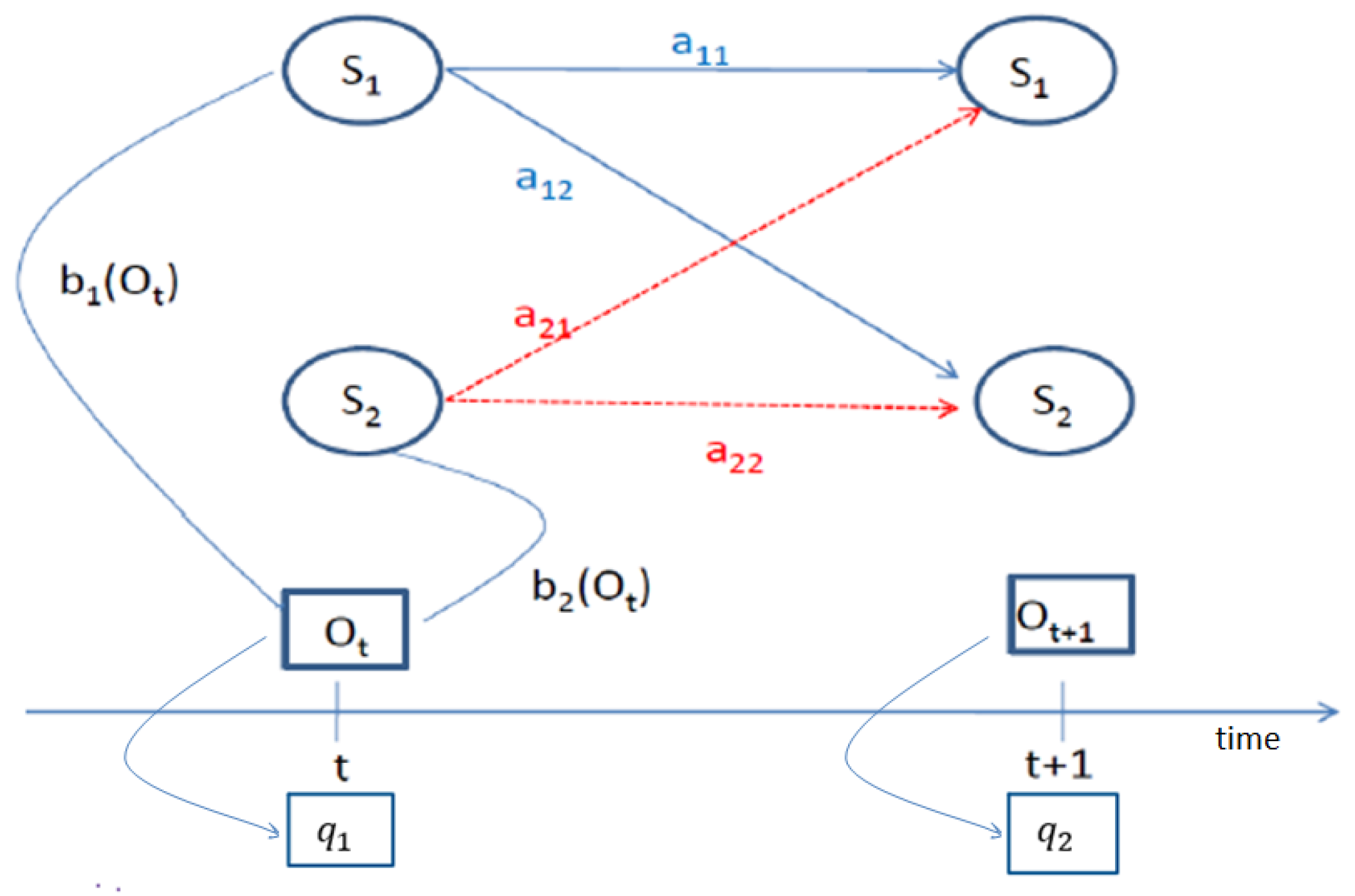
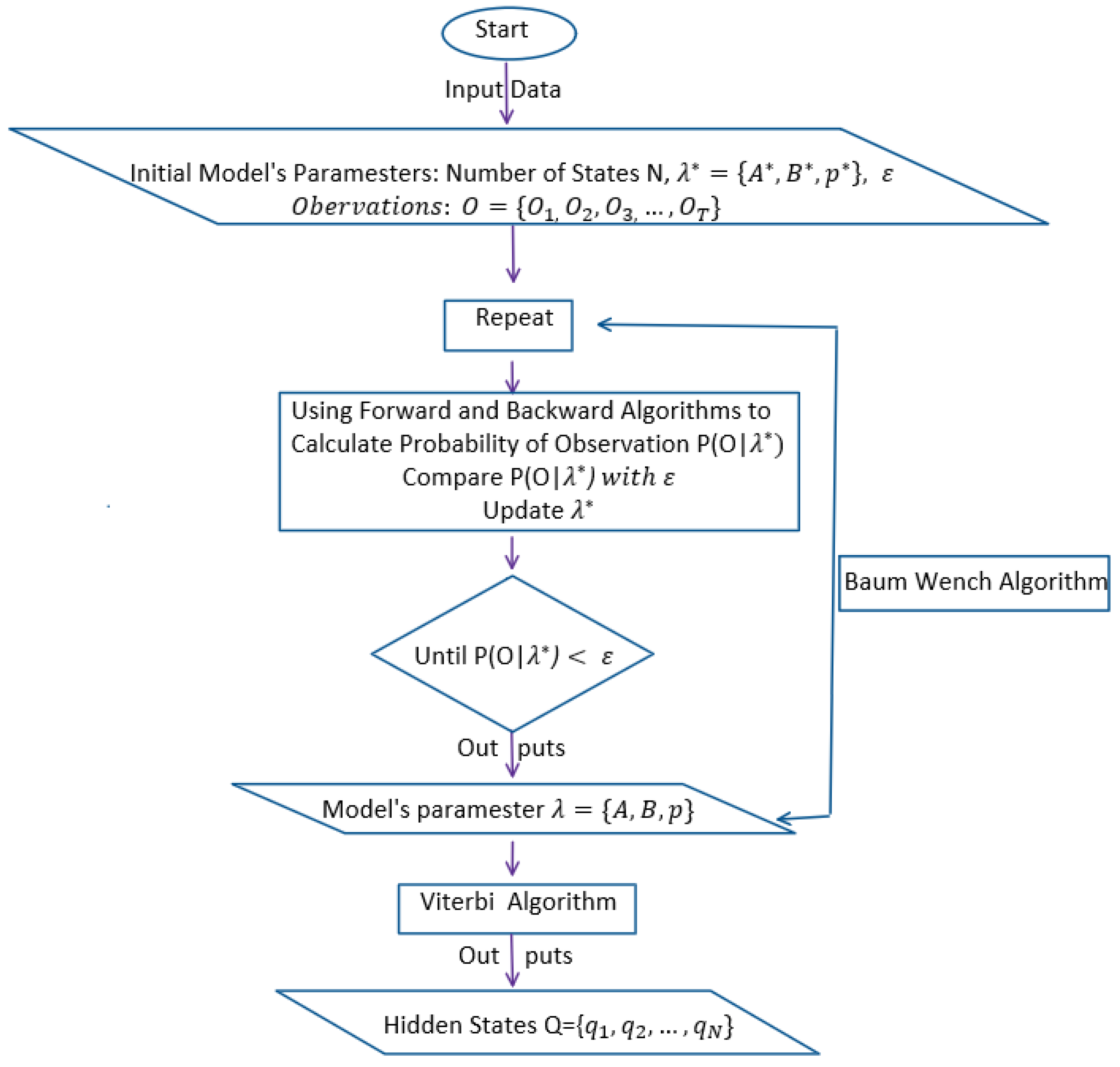
2. Hidden Markov Model
3. All Country World Index and Global Economic Indicators
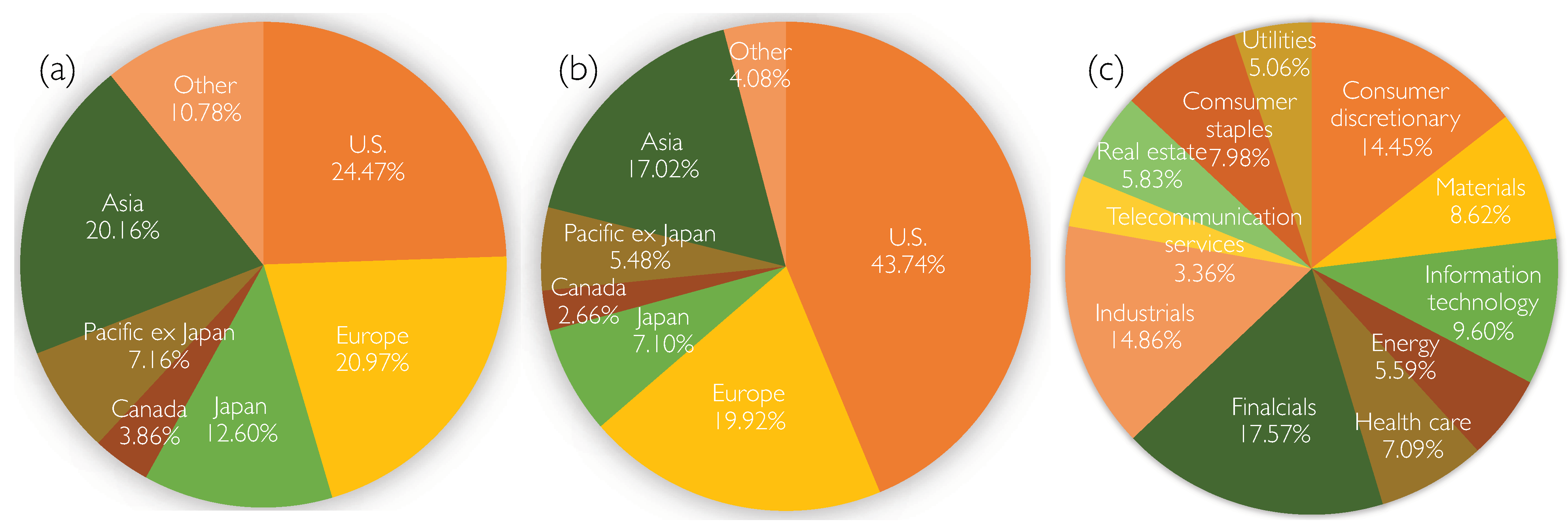
3.1. All Country World Index
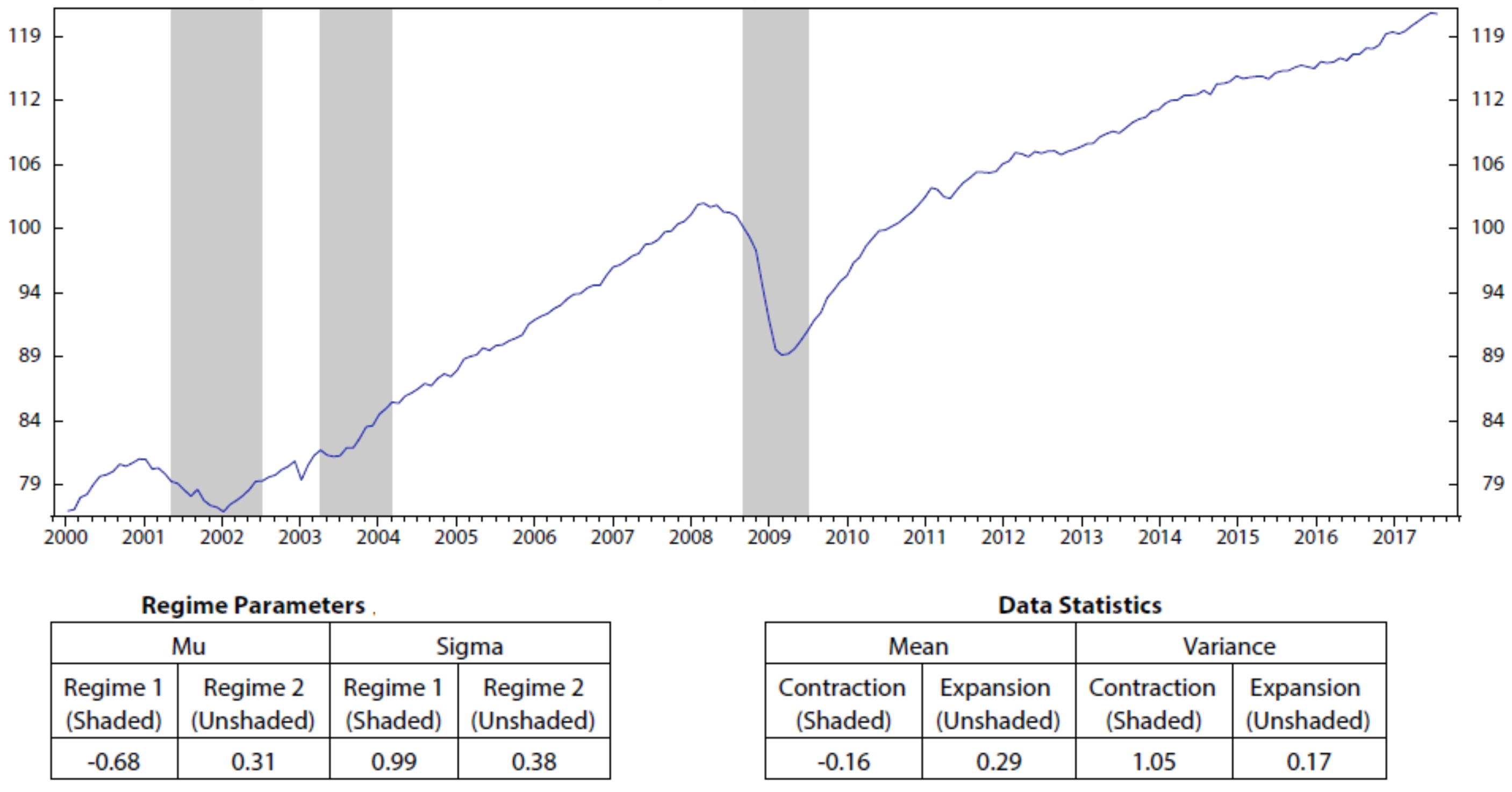
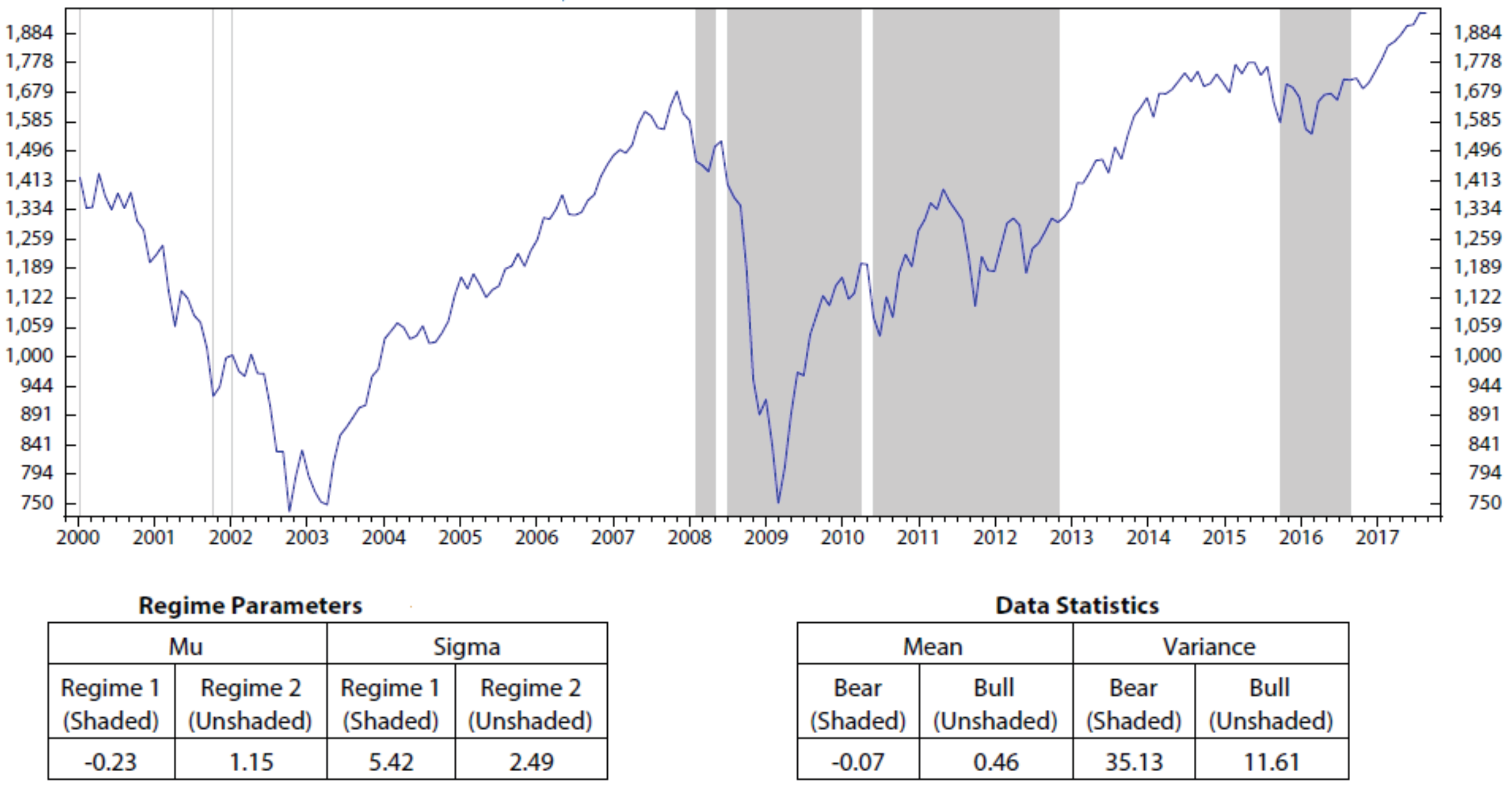
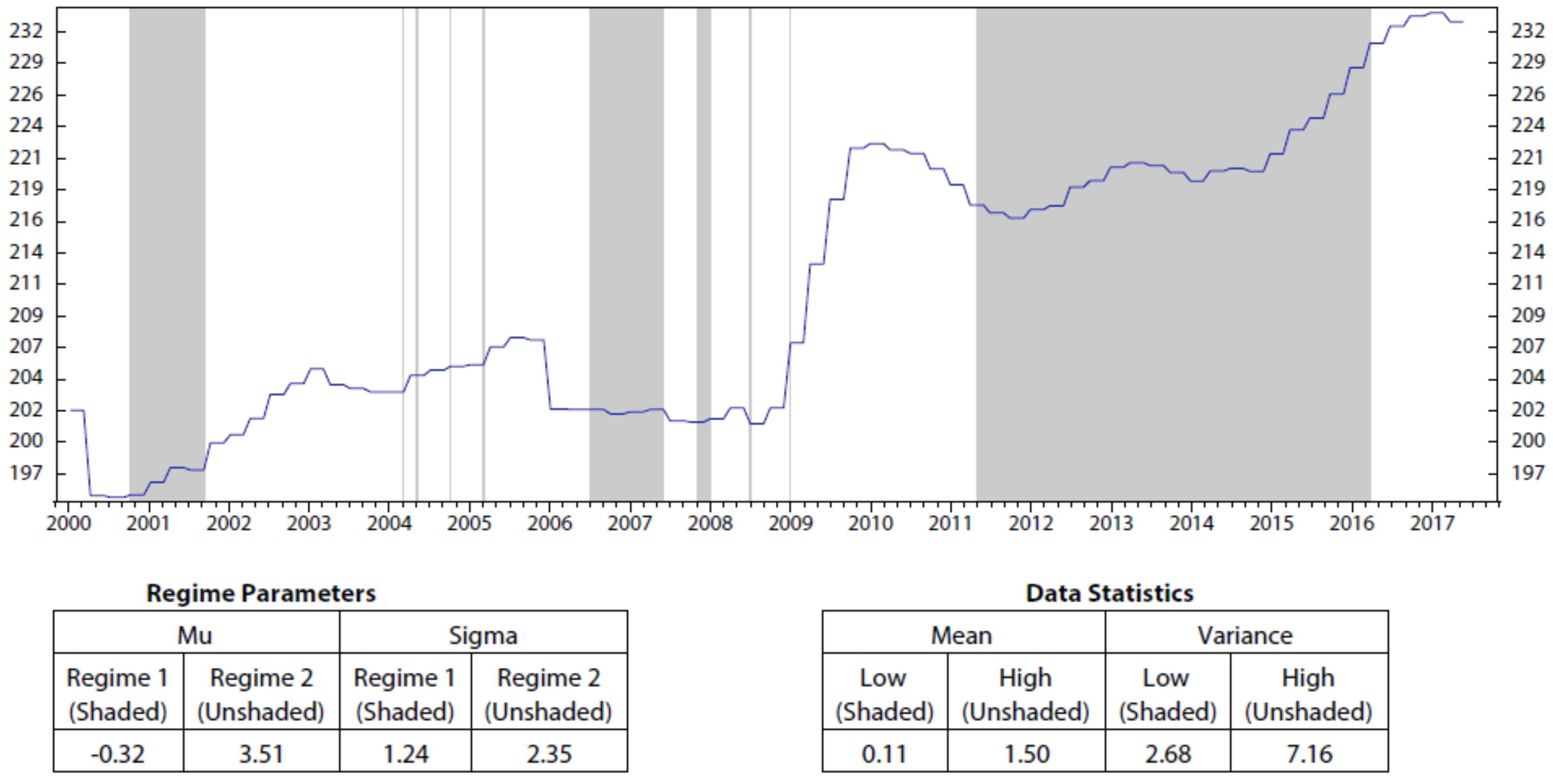
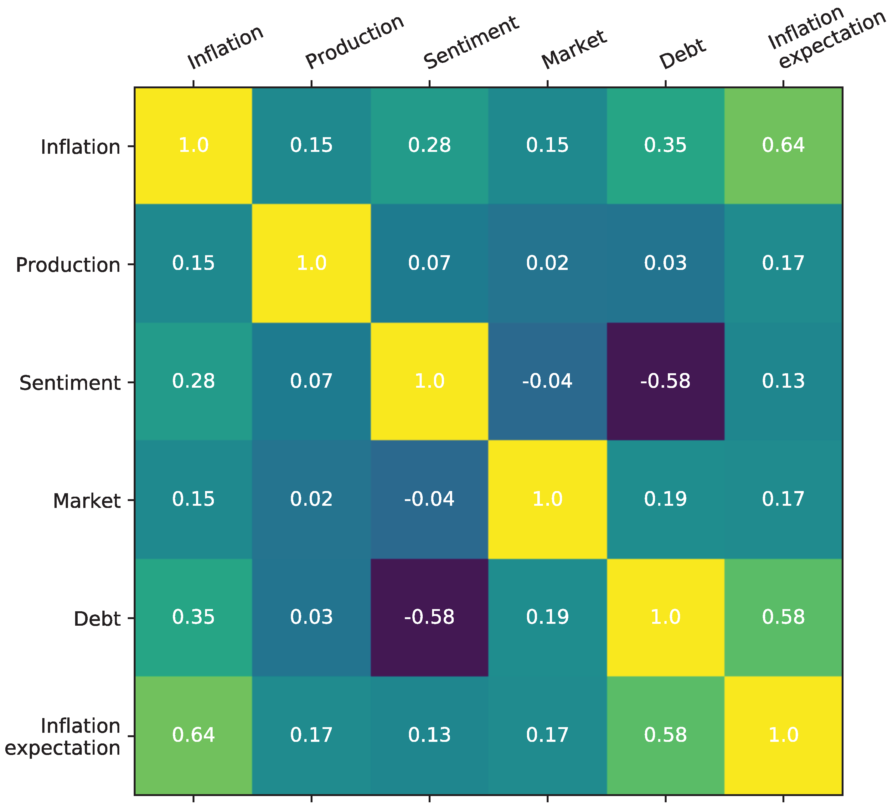
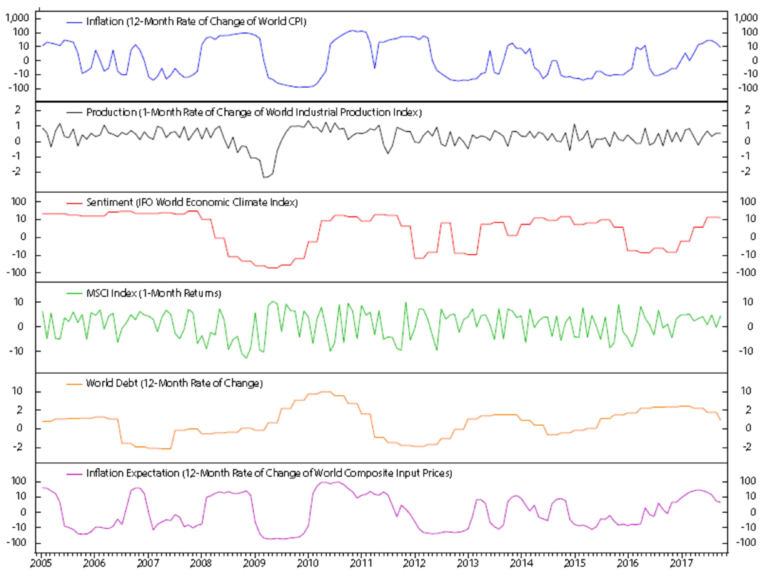
3.2. Global Economic Indicators
4. Stock Factors
5. Global Stock Selection Using HMM
5.1. Stock Factors Scoring
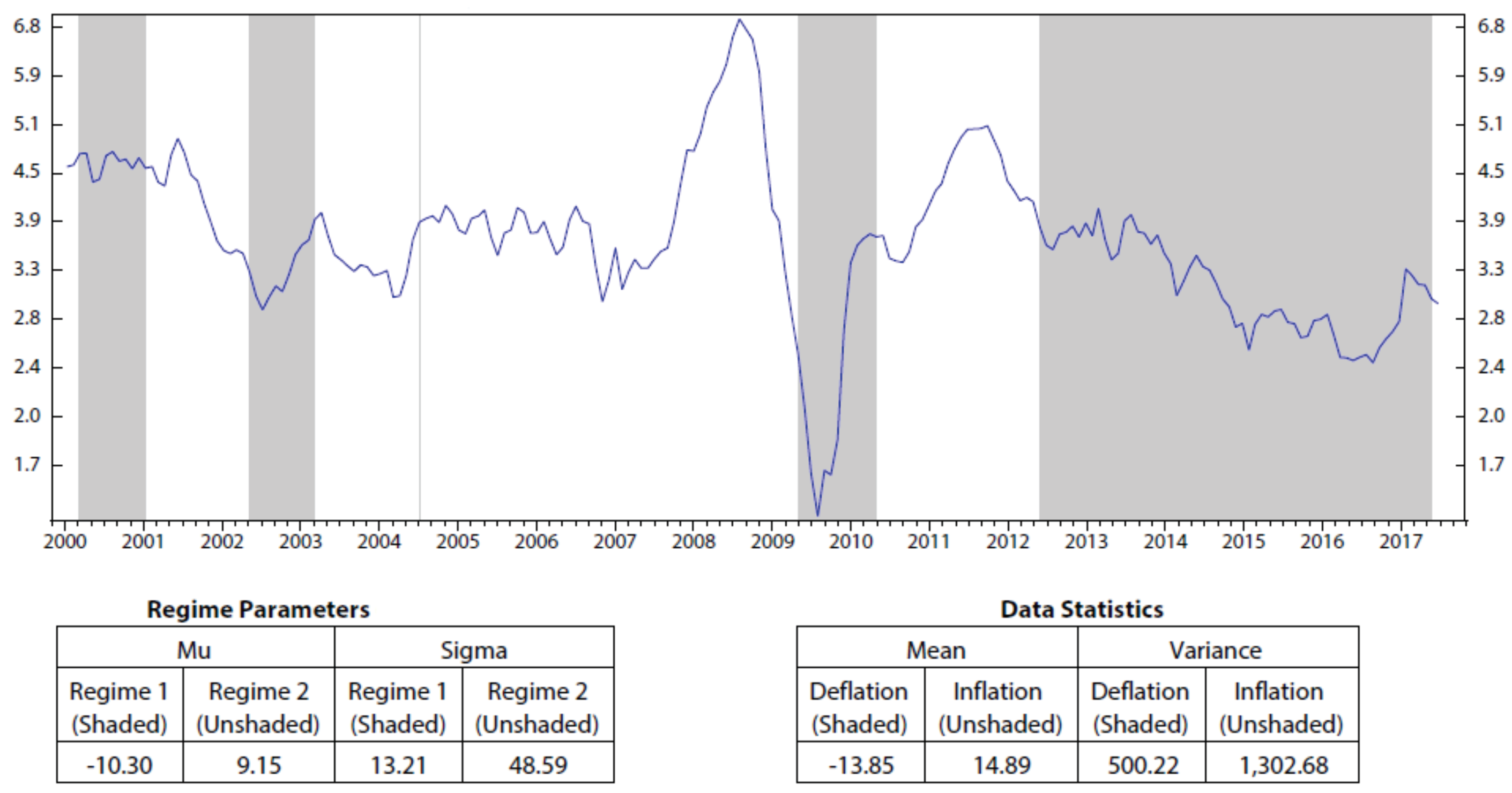
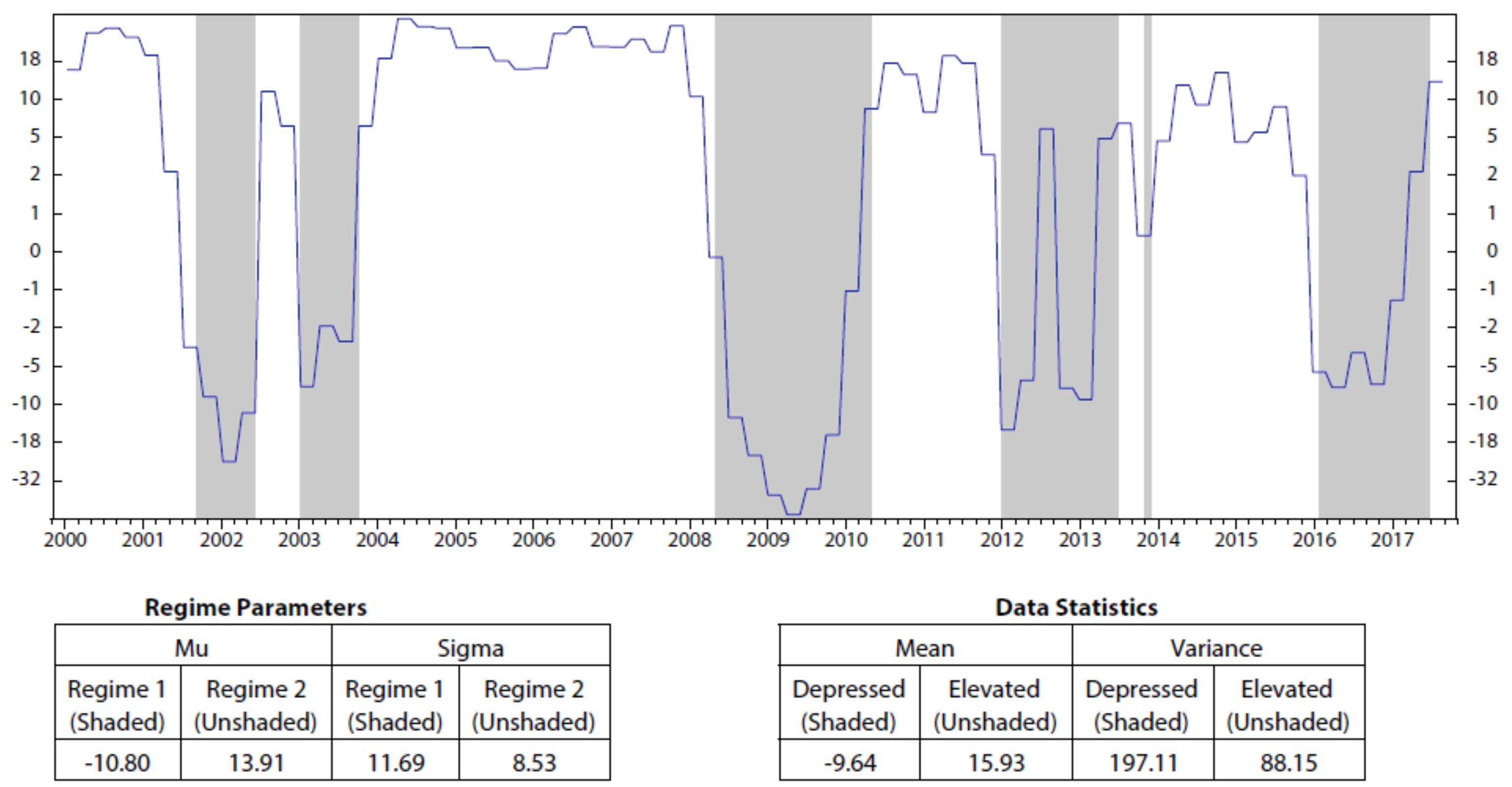
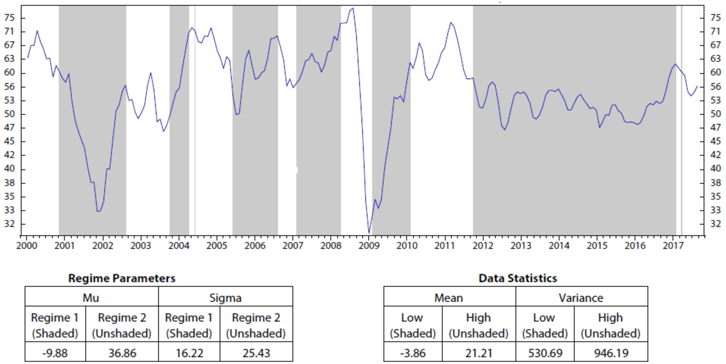
5.2. Regime Detection Using HMM
5.3. Stock Composition Scores
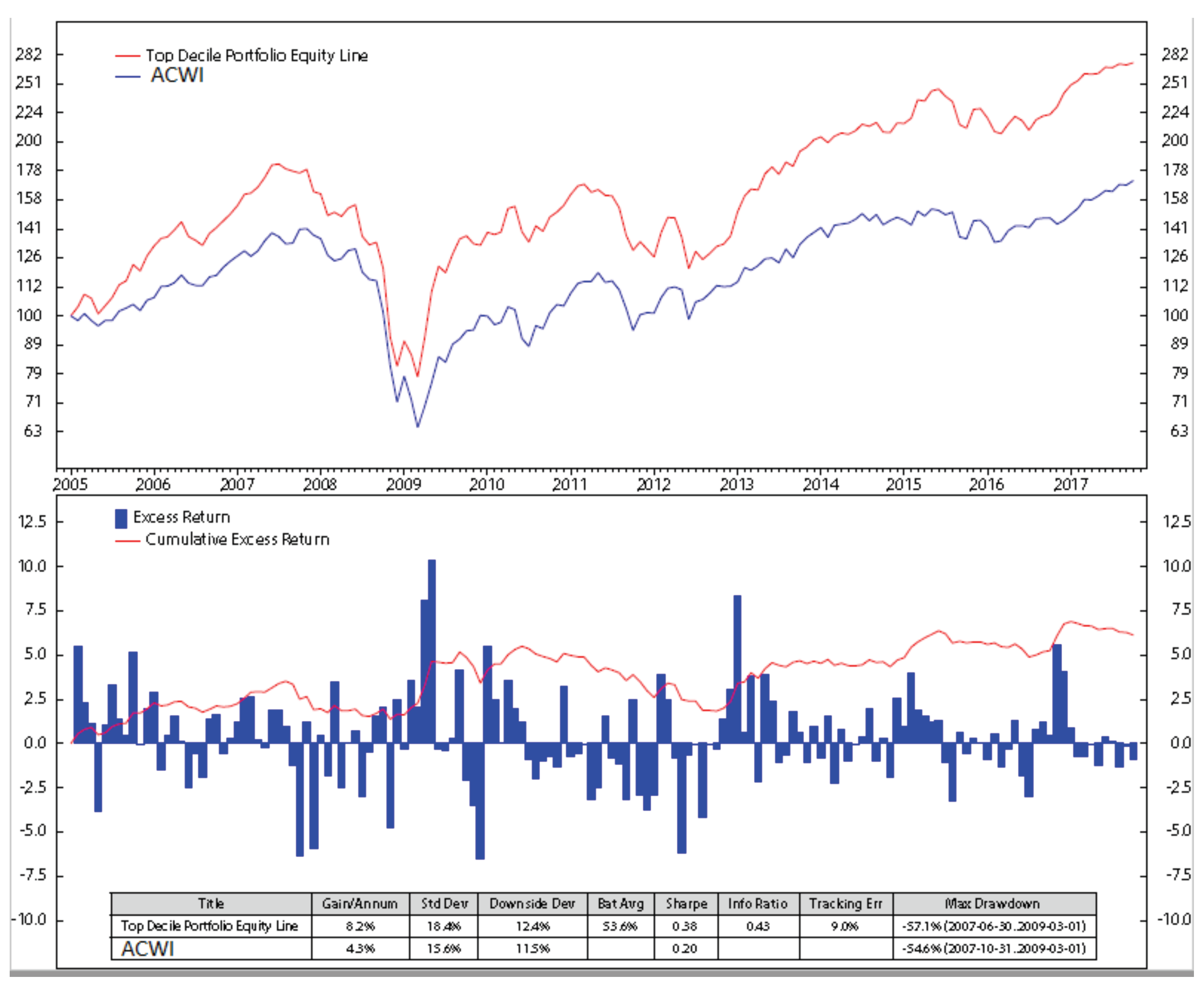
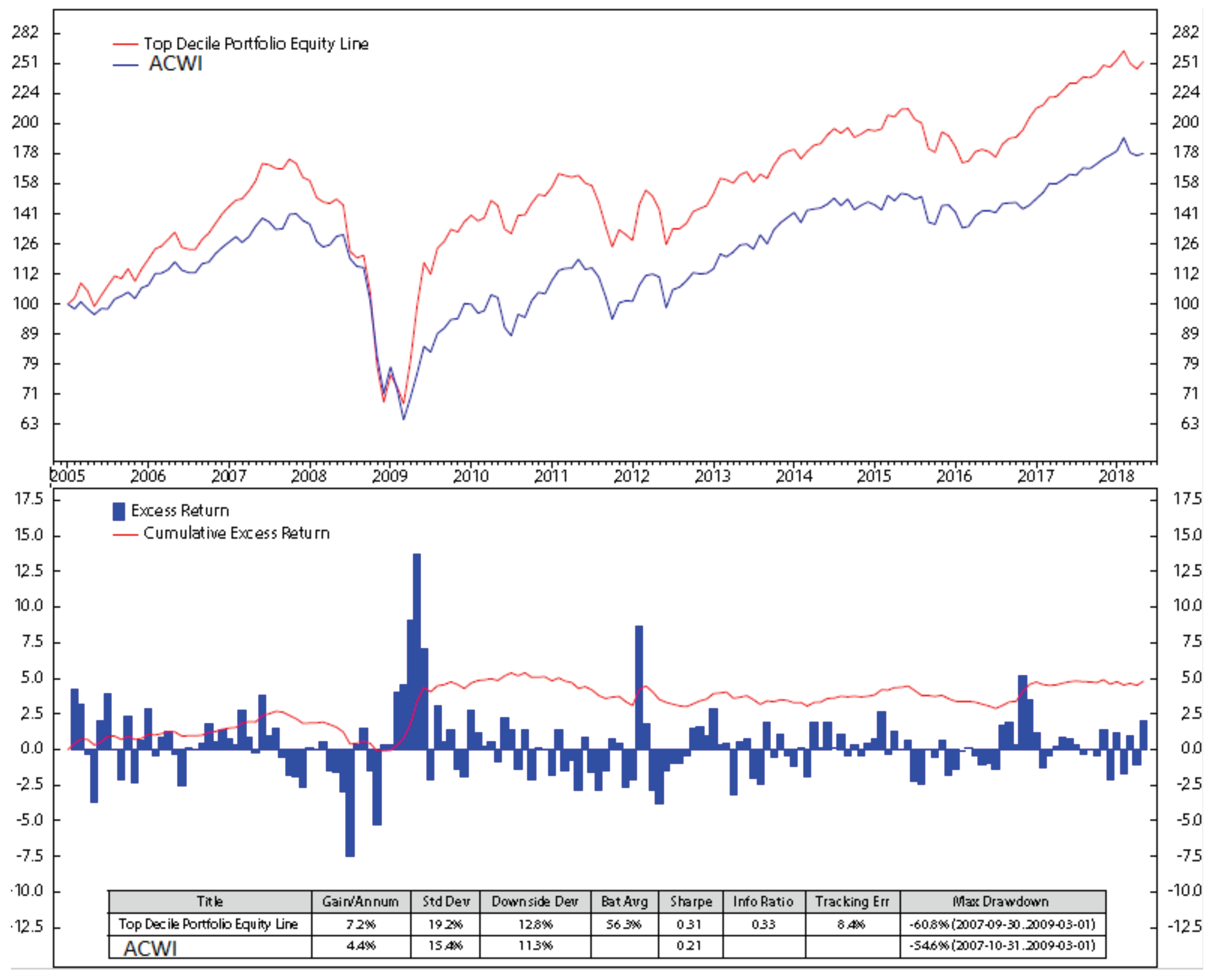
6. Results and Discussions
7. Conclusions
Author Contributions
Funding
Conflicts of Interest
Appendix A. Regime Detection Using HMM


Appendix B. Stock Portfolio Performances

References
- Alloway, T. 2019. JPMorgan Creates ’Volfefe’ Index to Track Trump Tweet Impact. Bloomberg. Available online: https://www.bloomberg.com/news/articles/2019-09-09/jpmorgan-creates-volfefe-index-to-track-trump-tweet-impact (accessed on 9 September 2019).
- Andriosopoulos, Dimitris, Michalis Doumpos, Panos M. Pardalos, and Constantin Zopounidis. 2019. Computational approaches and data analytics in financial services: A literature review. Journal of the Operational Research Society 70: 1–19. [Google Scholar] [CrossRef]
- Ball, Philip. 2013. Counting Google searches predicts market movements. Natute News. [Google Scholar] [CrossRef]
- Baum, Leonard, and Ted Petrie. 1966. Statistical inference for probabilistic functions of finite state Markov chains. Institute of Mathematical Statistics 37: 1554–63. [Google Scholar] [CrossRef]
- Baum, Leonard, Ted Petrie, George Soules, and Norman Weiss. 1970. A maximization technique occurring in the statistical analysis of probabilistic functions of Markov chains. Annals of Mathematical Statistics 41: 164–71. [Google Scholar] [CrossRef]
- Brown, Frank K. 1998. Chapter 35—Chemoinformatics: What is it and How does it Impact Drug Discovery. In Annual Reports in Medicinal Chemistry. Cambridge: Academic Press, vol. 33, pp. 375–84. [Google Scholar]
- Bunke, H., Markus Roth, and Ernst Günter Schukat-Talamazzini. 1995. Off-line cursive handwriting recognition using hidden markov models. Pattern Recognit. 28: 1399–1413. [Google Scholar] [CrossRef]
- de Prado, Marcos Lopez. 2018. Advances in Financial Machine Learning, 1st ed. Hoboken: Wiley. [Google Scholar]
- Engel, Thomas. 2006. Basic Overview of Chemoinformatics. Journal of Chemical Information and Modeling 46: 2267–77. [Google Scholar] [CrossRef] [PubMed]
- Fan, Alan, and Marimuthu Palaniswami. 2001. Stock selection using support vector machines. Paper presented at the International Joint Conference on Neural Networks, Washington, DC, USA, July 15–19; vol. 3, pp. 1793–98. [Google Scholar]
- Graham, Benjamin. 2003. The Intelligent Investor, revised ed. New York: HarperCollins. [Google Scholar]
- Hamilton, James. 1989. A New Approach to the Economic Analysis of Nonstationary Time Series and the Business Cycle. Econometrica 57: 357–84. [Google Scholar] [CrossRef]
- Hassan, Rafiul, and Baikunth Nath. 2005. Stock Market Forecasting Using Hidden Markov Model: A New Approach. Paper presented at 5th International Conference on Intelligent Systems Design and Applications, Wroclaw, Poland, September 8–10. [Google Scholar]
- Hondroyiannis, George, and Evangelia Papapetrou. 2001. Macroeconomic influences on the stock market. Journal of Economics and Finance 25: 33–49. [Google Scholar] [CrossRef]
- Huan, Tran Doan, Arun Mannodi-Kanakkithodi, and Rampi Ramprasad. 2015. Accelerated materials property predictions and design using motif-based fingerprints. Physical Review B 92: 014106. [Google Scholar] [CrossRef] [Green Version]
- Huang, Chien-Feng. 2012. A hybrid stock selection model using genetic algorithms and support vector regression. Applied Soft Computing 12: 807–18. [Google Scholar] [CrossRef]
- Idvall, Patrik, and Conny Jonsso. 2008. Algorithmic Trading: Hidden Markov Models on Foreign Exchange Data. Master’s Dissertation, Linköping University, Linköping, Sweden. [Google Scholar]
- Kavitha, G., A. Udhayakumar, and D. Nagarajan. 2013. Stock Market Trend Analysis Using Hidden Markov Models. arXiv arXiv:arXiv:1311.4771. [Google Scholar]
- Khan, Jawad, and Imran Khan. 2018. The Impact of Macroeconomic Variables on Stock Prices: A Case Study of Karachi Stock Exchange. Journal of Economics and Sustainable Development 9: 2222–55. [Google Scholar] [CrossRef]
- Kim, Chiho, Anand Chandrasekaran, Tran Doan Huan, Deya Das, and Rampi Ramprasad. 2018. Polymer Genome: A Data-Powered Polymer Informatics Platform for Property Predictions. Journal of Physical Chemistry C 122: 17575–85. [Google Scholar] [CrossRef]
- Kritzman, Mark, Sébastien Page, and David Turkington. 2012. Regime Shifts: Implications for Dynamic Strategies. Financial Analysts Journal 68: 3. [Google Scholar] [CrossRef]
- Lajos, Jaroslav. 2011. Computer Modeling Using Hidden Markov Model Approach Applied to the Financial Markets. Ph.D. Dissertation, Oklahoma State University, Stillwater, OK, USA. [Google Scholar]
- Levinson, S., L. R. Rabiner, and M. M. Sondhi. 1983. An introduction to the application of the theory of probabilistic functions of Markov process to automatic speech recognition. Bell System Technical Journal 62: 1035–74. [Google Scholar] [CrossRef]
- Li, Na, and Matthew Stephens. 2003. Modeling Linkage Disequilibrium and Identifying Recombination Hotspots Using Single-Nucleotide Polymorphism Data. Genetics 165: 2213–33. [Google Scholar] [PubMed]
- Li, Xiaolin, Marc Parizeau, and Réjean Plamondon. 2000. Training Hidden Markov Models with Multiple Observations—A Combinatorial Method. IEEE Transactions on PAMI 22: 371–77. [Google Scholar]
- Liu, Guang, and Xiaojie Wang. 2019. A new metric for individual stock trend prediction. Engineering Applications of Artificial Intelligence 82: 1–12. [Google Scholar] [CrossRef]
- Liu, Yi-Cheng, and I-Cheng Yeh. 2017. Using mixture design and neural networks to build stock selection decision support systems. Neural Computing and Applications 28: 521–535. [Google Scholar] [CrossRef]
- Humpe, Andreas, and Peter Macmillan. 2009. Can macroeconomic variables explain long-term stock market movements? A comparison of the US and Japan. Applied Financial Economics 19: 111–19. [Google Scholar] [CrossRef]
- Mamon, Rogemar S., and Robert J. Elliott, eds. 2007. Hidden Markov Models in Finance. New York: Springer, vol. 104. [Google Scholar]
- Markowitz, Harry. 1952. Porfolio selection. Journal of Finance 7: 77–91. [Google Scholar]
- Nenortaite, Jovita, and Rimvydas Simutis. 2004. Stocks’ Trading System Based on the Particle Swarm Optimization Algorithm. In Computational Science—ICCS 2004. Edited by M. Bubak, G. D. van Albada, P. M. A. Sloot and J. Dongarra. Poland: Springer, pp. 843–50. [Google Scholar]
- Nguyen, Nguyet, and Dung Nguyen. 2015. Hidden Markov Model for Stock Selection. Risks 3: 455–73. [Google Scholar] [CrossRef] [Green Version]
- Nguyen, Nguyet, Dung Nguyen, and Thomas Wakefield. 2018. Using the Hidden Markov Model to Improve the Hull-White Model for Short Rate. International Journal of Trade, Economics and Finance 9: 54–59. [Google Scholar] [CrossRef]
- Nguyen, Nguyet. 2017a. Hidden Markov Model for Portfolio Management with Mortgage-Backed Securities Exchange-Traded Fund. Technical Report. Schaumburg: Society of Actuaries. [Google Scholar]
- Nguyen, Nguyet. 2017b. An Analysis and Implementation of the Hidden Markov Model to Technology Stock Prediction. Risks 5: 62. [Google Scholar] [CrossRef] [Green Version]
- Nijam, Habeeb Mohamed, Smm Ismail, and Amm Musthafa. 2015. The Impact of Macro-Economic Variables on Stock Market Performance; Evidence from Sri Lanka. Journal of Emerging Trends in Economics and Management Sciences 6: 151–57. [Google Scholar]
- Pardo, Bryan, and William Peter Birmingham. 2005. Modeling form for on-line following of musical performances. Paper Presented at 20th National Conference on Artificial Intelligence, Pittsburgh, PA, USA, 9–13 July; pp. 1018–23. [Google Scholar]
- Preis, Tobias, Helen Susannah Moat, and Stanley H. Eugene. 2013. Quantifying Trading Behavior in Financial Markets Using Google Trends. Scientific Reports 3: 1684. [Google Scholar] [CrossRef] [Green Version]
- Rabiner, L. R., and B. H. Juang. 1992. Hidden Markov Models for Speech Recognition—Strengths and Limitations. In Speech Recognition and Understanding. Edited by P. Laface and R. De Mori. Berlin: Springer, pp. 3–29. [Google Scholar]
- Sanborn, B., D. Nguyen, and T. Nguyen. 2017. Global Factor-Based Investing—Opportunities, Risks, and Implementation. Technical Report: Ned Davis Research-NDR Explorer-Insights. [Google Scholar]
- Satish, L., and B. I. Gururaj. 1993. Use of hidden Markov models for partial discharge pattern classification. IEEE Transactions on Electrical Insulation 28: 172–82. [Google Scholar] [CrossRef]
- Thawornwong, Suraphan, and David Enke. 2004. Forecasting Stock Returns with Artificial Neural Networks. In Neural Networks in Business Forecasting. Edited by G. Peter Zhang. Hershey: IRM Press. [Google Scholar]
- Yoon, Byung-Jun. 2009. Hidden Markov Models and their Applications in Biological Sequence Analysis. Current Genomics 10: 402–15. [Google Scholar] [CrossRef] [Green Version]
- Yu, Lean, Lunchao Hu, and Ling Tang. 2016. Stock Selection with a Novel Sigmoid-Based Mixed Discrete-Continuous Differential Evolution Algorithm. IEEE Transactions on Knowledge and Data Engineering 28: 1891–904. [Google Scholar] [CrossRef]


| Variable | Notation |
|---|---|
| Length of observation data | T |
| Number of states | N |
| Number of symbols per state | M |
| Observation sequence | |
| Hidden state sequence | |
| Possible values of each state | |
| Possible symbols per state | |
| Transition matrix | , where |
| Vector of initial probability of being in state (regime) at time | , where |
| Observation probability matrix | , where and |
| Indicator | Name | Source | Data Used |
|---|---|---|---|
| Inflation | Consumer price index | International Monetary Fund | Yearly change |
| Production | Industrial production | Haver Analytics | Monthly change |
| Sentiment | Economic climate index | Ifo Institute for Economic Research | Original series |
| Market | MSCI world index | Morgan Stanley, Capital International | Monthly change |
| Debt | Public and private non-financial debt | Bank for International Settlements | Monthly change |
| Inflation expectation | Manufacturing purchasing managers’ index | Haver Analytics | Yearly change |
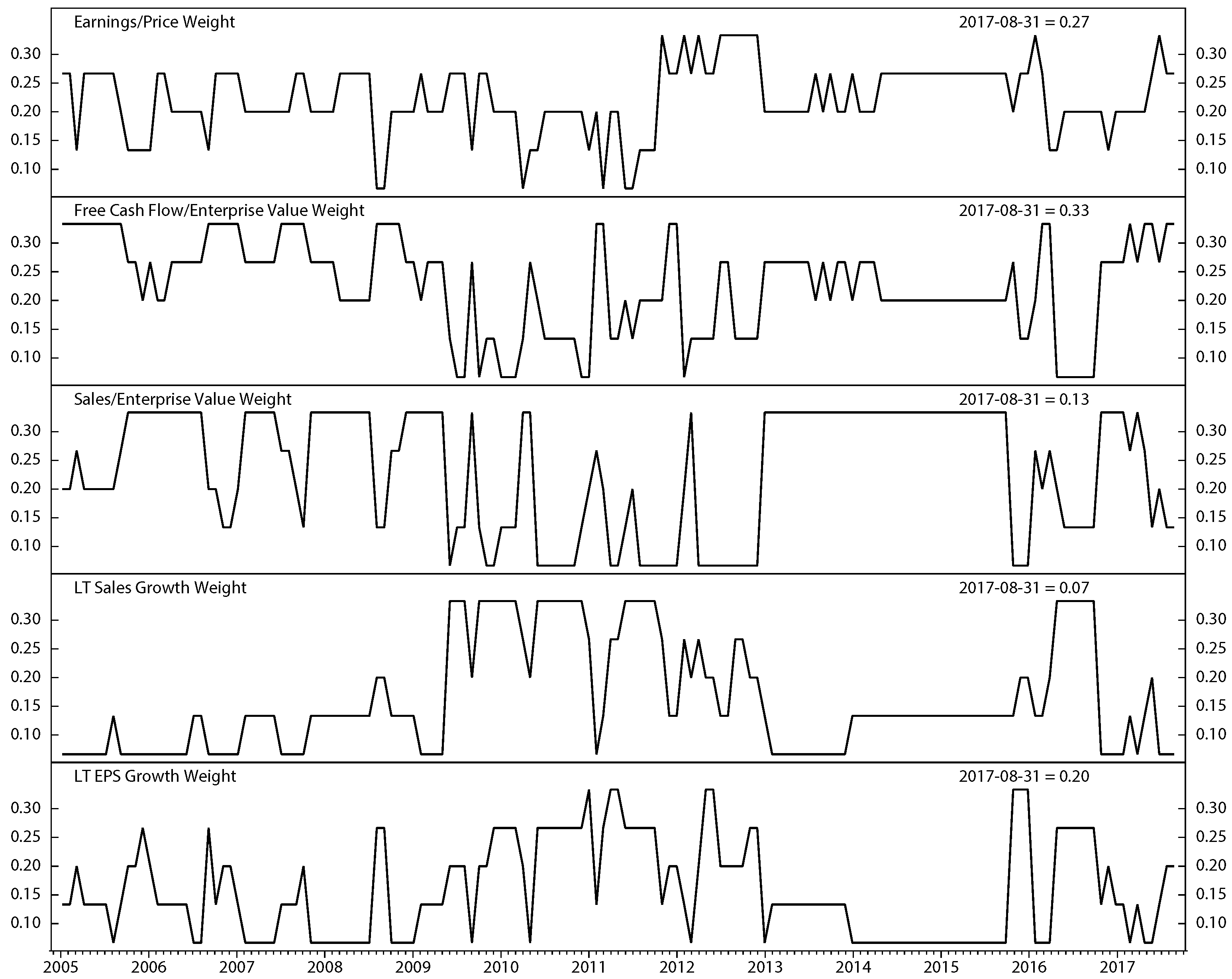
| Stock Factor | Definition and Meaning |
|---|---|
| Free cash flow/enterprise value | Operating cash flow subtracted by the sum of cash dividends plus capital expenditures divided by the market value of equity plus debt. |
| Earning/price | Earnings accumulated over the trailing twelve months of the stock divided by the weekend price. A higher number indicates a greater value for each unit of earnings, which tends to drive a higher stock return. |
| Sale/enterprise | Sales accumulated over the trailing twelve months of the stock divided by the market value of equity plus debt (enterprise value). A higher sale/enterprise value signifies that each unit of a stock’s value is used to generate more sales, which normally leads to higher stock return. |
| Long-term sale growth | The projected long-term growth rate of sales based on a five-year moving regression trend line. A high sale growth rate normally leads to a higher future returns. |
Publisher’s Note: MDPI stays neutral with regard to jurisdictional claims in published maps and institutional affiliations. |
© 2020 by the authors. Licensee MDPI, Basel, Switzerland. This article is an open access article distributed under the terms and conditions of the Creative Commons Attribution (CC BY) license (http://creativecommons.org/licenses/by/4.0/).
Share and Cite
Nguyen, N.; Nguyen, D. Global Stock Selection with Hidden Markov Model. Risks 2021, 9, 9. https://doi.org/10.3390/risks9010009
Nguyen N, Nguyen D. Global Stock Selection with Hidden Markov Model. Risks. 2021; 9(1):9. https://doi.org/10.3390/risks9010009
Chicago/Turabian StyleNguyen, Nguyet, and Dung Nguyen. 2021. "Global Stock Selection with Hidden Markov Model" Risks 9, no. 1: 9. https://doi.org/10.3390/risks9010009
APA StyleNguyen, N., & Nguyen, D. (2021). Global Stock Selection with Hidden Markov Model. Risks, 9(1), 9. https://doi.org/10.3390/risks9010009