1. Introduction
The recent outbreak of COVID-19 reminds us that epidemics raise not only sanitary but also financial issues. There is a clear and growing need for covering the epidemic risk and for developing analytically tractable models. In this article, we propose a new deterministic model in which the contagion rate is inversely proportional to time instead of to the susceptible population. This model presents a great analytical tractability and replicates the first wave of COVID-19 in Belgium, Germany, Italy and Spain. In this framework, we infer a closed-form expression for the fair premium rate of an insurance plan covering healthcare expenses of infected persons and providing a lump sum capital payment in case of death.
The deterministic model is next extended in two different directions. In the first one, the time scale is random and ruled by a process called subordinator. Using a gamma process as stochastic clock preserves the analytical tractability and randomizes the dynamic of the pandemic. In the second extension, the evolution of the infectious population is noised by a Brownian diffusion and a jump process.
Multiple contributions are presented in this article. The literature on mathematical modeling of epidemic is abundant, but most of the existing solutions, as compartment models, do not provide any analytical expression for the evolution of populations in each compartment. The valuation of an epidemic-linked insurance requires one to calculate integrals of infected and susceptible population sizes and is therefore computationally intensive. The three models proposed in this article do suffer from this problem and have a high level of analytical tractability for actuarial applications. Furthermore, estimating their parameters does not pose any problem, and their empirical explanatory power is comparable to the one of the susceptible-infected-recovered (SIR) approach. Finally, the jump diffusion extension allows one to simulate realistic random epidemic scenarios and to value reinsurance treaties.
We first present an overview of previous research. This is followed by the introduction of the deterministic model that is compared to the susceptible-infected-recovered (SIR) approach.
Section 4 studies the valuation of an insurance plan with healthcare and death benefits. The model is fitted to COVID-19 datasets for Belgium, Germany, Italy and Spain in the next section.
Section 6 introduces the first stochastic variant of this model, based on a random gamma clock. The valuation of reinsurance treaties is developed in the next paragraph and the time-changed model is estimated in
Section 8.
Section 9 and
Section 10 explore the features of the jump diffusion model. Finally, we propose an estimation method and fit the model to COVID-19 datasets.
2. Overview of Previous Research
Communicable diseases have always been an important part of human history as underlined by
Smith (
2017), who reviews their nature and proposes a brief history of pandemics. He also introduces the mathematical models used to evaluate the risk that pandemics pose to human populations. Another detailed survey of these quantitative models, including future perspective, is available in
Brauer (
2017).
The reference model in epidemiology is the susceptible-infected-recovered (SIR) model proposed by
Kermack and McKendrick (
1927). Various disease outbreaks, including the SARS epidemic of 2002–2003, the concern about a possible H5N1 influenza epidemic in 2005, the H1N1 influenza pandemic of 2009 and the Ebola outbreak of 2014 have reignited interest in epidemic models, beginning with the reformulation of the Kermack–McKendrick model by
Diekmann et al. (
1995). In the SIR, the population is homogeneous, whereas in reality, an epidemic spreads differently according to factors like the age or susceptibility to infection. It is then necessary to follow the secondary infections in the subpopulations separately; this is done through the next-generation matrix as explained by
Diekmann et al. (
1990) and
Van den Driessche and Watmough (
2002).
Anderson and May (
1979) extended the SIR model by considering the host population as a dynamic variable rather than a constant.
Tchuenche et al. (
2007) studied the stability of a SIR model with a time delay in the contagion dynamic. Under the assumption that all individuals are susceptible, they showed that the endemic equilibrium is stable. Similarly,
Zhang and Wang (
2013) studied a nonautonomous SIRS epidemic model with time delay.
The SIR model has been extended to multiple compartments with labels such as M, S, E, I and R that are often used for the epidemiological classes. The class M contains infants with passive immunity inherited at birth. After that, the infant moves to the susceptible class S. When a susceptible individual has adequate contact with an infected individual such that transmission occurs, then the susceptible individual enters the exposed class E of those in the latent period, who are infected but not yet infectious. After the latent period ends, the individual enters the class I of infectious. We refer the reader to
Hethcote (
2000) for a comparison of MSEIR and SEIR models for various diseases, including measles in Niger and pertussis in the United States.
Drawing conclusions from mathematical models raises the question of the origin of data and of methodological best practices.
Walters et al. (
2018) reviewed the literature, highlighting common approaches and good practice and identifying research gaps. They extracted information from 78 records and found that most epidemiological data come from published journal articles, population data come from a wide range of sources and travel data mainly come from statistics or surveys.
Rhodes et al. (
2020) traced how models can be investigated as matters of correspondence and enactment in relation to their social and policy contexts.
At the beginning of a disease outbreak, there is a small number of infectious individuals and the transmission of infection is a stochastic event depending on the pattern of contacts between members of the population. The
Watson and Galton (
1874) process was one of the first approaches to successfully described this pattern. An alternative consists of introducing random noise into differential equations defining each compartment.
Zhang and Wang (
2013) explored this alternative and studied the asymptotic behavior of SIR model with Brownian noise and a jump process. The stochastic model containing a standard Brownian motion was studied by
Caraballo and Colucci (
2017).
Caraball and Keraani (
2018) explored the features of a stochastic SIR model with a fractional Brownian motion. The book by
Daley and Gani (
1999) contains an account of some of the more recent extensions.
In actuarial sciences, the literature on epidemics model is rather scarce.
Jia and Tsui (
2005) proposed and estimated a compartment model for severe acute respiratory syndrome (SARS) data.
Chen and Cox (
2009) employed the theory of real options and considered a regime-switching process for modeling the number of infected individuals.
Feng and Garrido (
2011) quantified the risk of infection with a classical epidemiological compartment model. They formulated financial arrangements between an insurer and insured using actuarial methodology and applied their framework to the SARS epidemic in 2003.
Gathy and Lefèvre (
2009) and
Lefevre and Utev (
1999) proposed extensions of deterministic compartment models and provided additional tools to account for randomness in epidemiological dynamics. Based on a Markov chain formulation of the susceptible-infected-recovered (SIR model),
Lefèvre et al. (
2017) developed a recursive method to calculate the cost components and the corresponding premium levels. More recently,
Clara-Rahola (
2020) proposed two distinct exponential models for the infection rate before and after lockdown. The fit to data from China, Spain, South Korea and Italy revealed that a crossover point between pre- and postlockdown infection rates is found one week after lockdown, which, in turn, is the average COVID-19 incubation period.
3. A Deterministic Epidemic Model
We consider a population of size
hit by an epidemic disease at time 0. We propose to model the number of infectious persons at time
, denoted by
, by the following relation:
where
. This function is the product of two terms. The first one is an exponential decreasing function,
, whereas the second one is an increasing function. The number of infectious decreases exponentially with a rate
. The parameter
is the recovery rate from the disease, whereas
is assumed to be the death rate of infected persons. The average duration before recovery is then
. At time 0, the initial number of infected individuals is equal to
. In order to understand the role played by the parameter
in the dynamics of infectious population, we differentiate Equation (
1):
This differential equation reveals that the initial contagion rate per capita is equal to
. This is a decreasing function to 0 when
. Empirical tests in following sections emphasizes that Equation (
2) explains the evolution of the first wave of COVID-19 in Belgium, Germany, Spain and Italy.
This model slightly differs from the susceptible-infected-recovered (SIR) model developed by
Kermack and McKendrick (
1927), which is a standard in the literature. In the SIR model, the evolution of the epidemics is described by the ordinary differential equations (ODEs):
where
and
is the number of persons that are susceptible to be infected at time
t. As in our model,
and
are the recovery and mortality rates, respectively. The contagion rate per capita in the SIR is proportional to the population of susceptible,
, whereas it is a function of time,
, in the approach proposed in this article. This assumption allows us to obtain the closed form expression (
2) for the infectious populations. This is the greatest benefit of this model compared to the SIR that does not admit analytical solutions for the system (
3). In actuarial applications developed in following sections, we have to integrate
. Therefore, having an analytical formula allows us to avoid numerical integration of an ODE numerical solution and propagation of numerical errors. Furthermore, the model (
2) is easily extended to stochastic frameworks, as detailed in following sections.
The basic reproduction number,
, is defined as the average number of secondary cases arising from a typical primary case. Under the assumption that the population of susceptible is large, we have
and the basic reproduction number of the SIR model is
. In our model, the reproduction number is instead a function of time equal to
. The time-varying
allows us to take into account the impact of preventive measures to curb the epidemic, such as a lockdown or the wearing of masks. The empirical analysis of the next section confirms that this approach offers a better fit than the SIR model. Our model presents other interesting features. In particular, the peak of the epidemic is known and obtained by canceling the first order derivative of Equation (
1):
Combining Equations (
1) and (
4) allows us to evaluate the size of the infected population when the peak is reached:
Since the population of infectious persons may not exceed
, we infer the necessary conditions
As
is the mortality rate, the total number of deaths up to time
t is a function, denoted by
, that is solution of the ordinary differential equation:
Under the assumptions that recovery does not not provide a protective immunity and that there is no entry into or departure from the population, the size of the population of susceptible, denoted by
, is then solution of the following ODE:
By construction, the population of susceptible growths when infected individuals recover from the disease and is decreased by the number of new contaminated. As we do not consider new entrants in the population, the sum of the number of susceptible individuals, infected individuals and deaths remains constant and equal to
:
4. Actuarial Valuation of an Insurance Plan
In the same spirit as
Feng and Garrido (
2011), we consider an infectious disease insurance plan that collects premiums in the form of continuous annuities from susceptibles, as long as they are healthy. The premium rate is assumed constant and noted
p. Collected premiums cover medical expenses which are continuously reimbursed for each infected policyholder during the period of treatment. The benefit rate is noted
b. The plan terminates when the individual recovers or dies from the disease. In case of death, a lump sum benefit,
c, is paid.
The risk-free rate is constant and denoted by
r. If the insurance plan covers the whole population, premium, benefit rates and lump sum death capital must ensure the financial equilibrium of the plan. Under the assumption that the plan starts at time 0 and finishes at time
T, discounted premiums have to cover all discounted benefits:
As stated in the previous section, the discounted integral of admits a closed-form expression.
Proposition 1. For , we have that:where and is the gamma lower incomplete function. Proof. Using Equation (
1), we develop the integral as follows:
and we perform a change of variable
in order to rewrite the integral:
From the definition of the gamma incomplete function, we directly obtain Equation (
10). □
From this last proposition, we immediately infer the expressions of , and .
Corollary 1. The cumulated number of deceases caused by the epidemic at time is equal to If , the second term on the right-hand side of Equation (9) is: The size of the population of susceptible at time is deduced from the relation : The next proposition reports the closed-form expression for the premium rate solution of Equation (
9).
Proposition 2. For the benefit rate , the fair premium rate that ensures the actuarial equilibrium of the plan is given bywhere the denominator is equal to: Proof. From Equation (
13), we infer that
The first integral on the right-hand side is equal to
whereas
is provided by Equation (
10). From Equation (
11), we infer that the integral of the discounted number of deaths is:
Integrating by parts leads to the following result:
The integral in this last expression may also be reformulated in terms of an incomplete lower gamma function:
Combining these results leads to Equation (
15) and the fair premium comes from the actuarial equilibrium equation. □
5. Empirical Illustration
We fit the model to data about the COVID-19 outbreak in Belgium, Germany, Italy and Spain. The first three countries are selected because they have reported the highest death rates in Europe during the 2020 first wave of COVID-19. In comparison, Germany has better managed the spread of the virus but the distribution of infected individuals over time has decreased at a lower pace than other countries considered in this study. We use the datasets from the library “coronavirus
1” in R which provides daily time-series of the number of deaths and detected cases of COVID from the beginning of 2020 up to the end of July. We choose as starting date the day when the number of confirmed cases passes above a threshold set to 0.005% of the total population of the country. As the model is designed for modeling a single epidemic wave, the ending date is set to the 15th of June 2020, which corresponds to the end of the lockdown period in the considered countries.
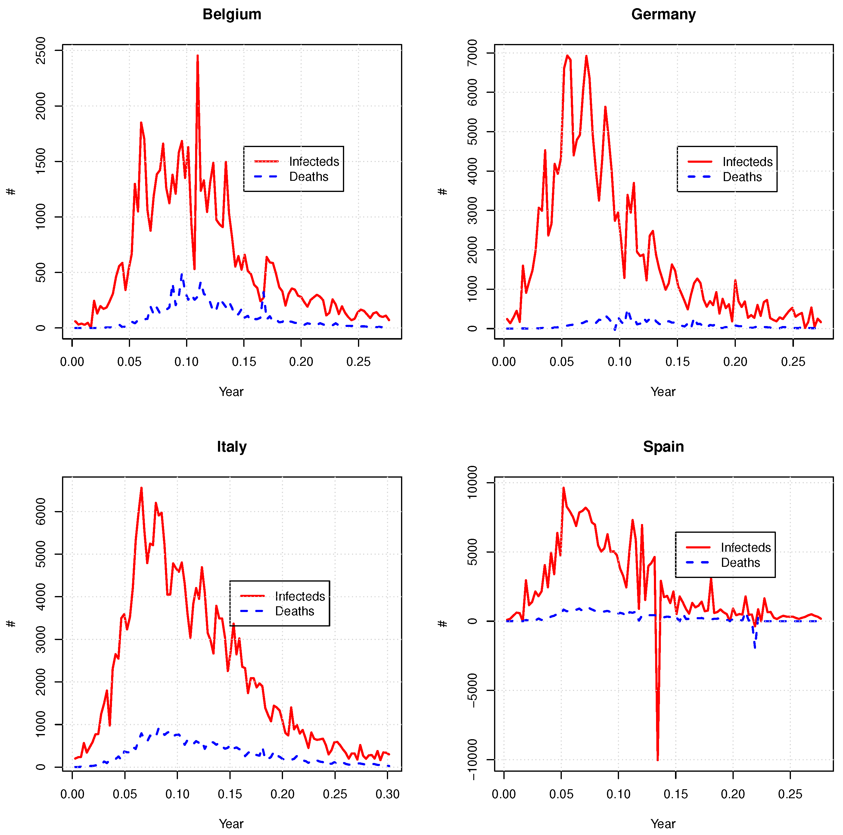
Figure 1 shows these time series and
Table 1 reports some statistics of the datasets. For Spain, the number of confirmed cases or deaths is negative for a few days. This is due to retrospective corrections.
Both the SIR and our model aim to describe the evolution of the number of infected persons,
. As the data sets only report new confirmed cases, we assume that contaminated individuals remain infected, on average, for 12 days, which is slightly less than the duration of the quarantine imposed, e.g., in Belgium (14 days) after being in touch with a contaminated person. If
is the time series of observations and
is the number of days, parameters are obtained by a weighted least-square minimization:
where
is the value of
at time
As the impacts of
and
on
are indistinguishable, we first estimate their sum. The annualized mortality rate is estimated as the ratio of the total number of deaths on the cumulated number of infecteds forecast by the model, multiplied by 365. Given that the COVID testing was far from being generalized in March, it is likely that the number of infected cases was higher than the one reported. In order to take this into account in the estimation procedure, more importance is granted to most recent daily observations as follows:
These weights are chosen in order to obtain the best compromise fitting both the tail and the peaks of the
curve. The results of the calibration procedure are reported in
Table 2.
We benchmark the capacity of Equation (
1) to model the evolution of the infected population with the SIR model, fitted by least-square minimization. Our numerical experiments reveals that the SIR model fails to replicate the curve of
. The only way to fit this model consists to consider that
is also a parameter. Parameter estimates are reported in
Table 3.
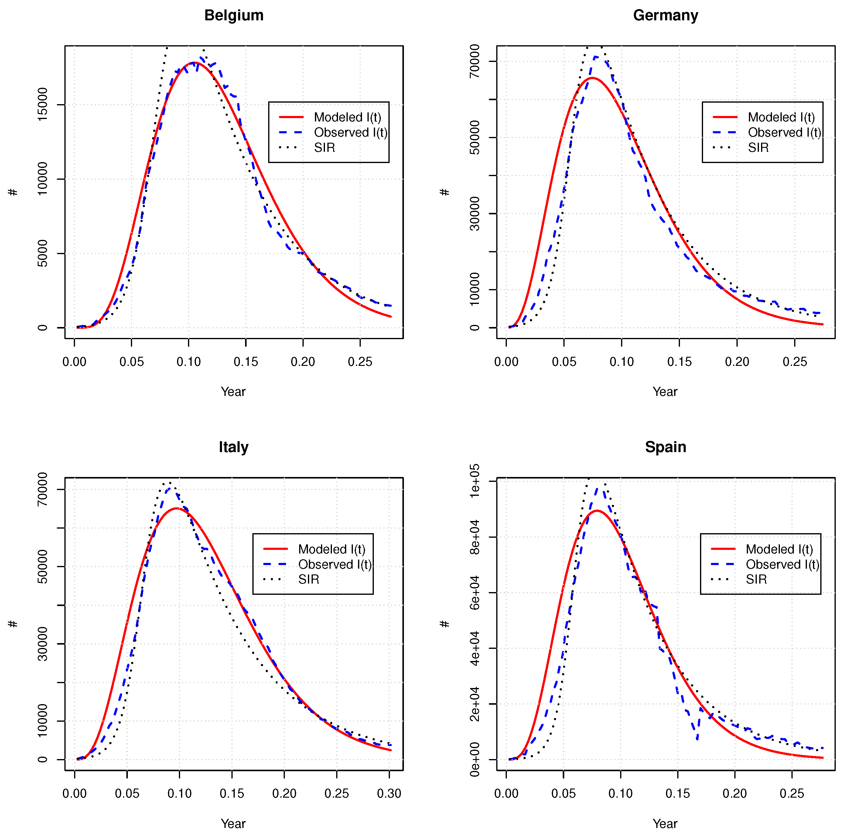
Figure 2 compares observed to forecast
with our and SIR models. The SIR offers at a first sight an excellent fit but considering that
is adjustable is hard to justify. Furthermore, the adjusted
are considerably smaller than the real size of considered populations. This confirms that our approach is a reliable alternative compared to the SIR model.
Next, we use parameter estimates in order to evaluate the fair premium rates of an insurance plan, such as described in
Section 4. Two cases are considered. In the first one, collected premiums cover exclusively medical expenses. An allowance of 1000 EUR per day is paid during the treatment (
365,000 EUR on a yearly basis). The second plan covers exclusively the death risk: a lump sum capital of 200,000 EUR is paid at the decease of an infected patient. The duration of both plans is six months and the risk-free rate is set to 2%.
Table 4 and
Table 5 report the fair premium rates calculated with our approach and the SIR model, respectively, for Belgium, Germany, Italy and Spain. We also test the sensitivity of these rates to variations of parameters. Per country, premium rates computed with our approach or the SIR model are similar. The premium rates for both benefits (62.38 EUR and 42.35 EUR per year) for Germany are the lowest due to the low number of confirmed cases and deaths reported by this country. The death coverage is the most expensive for Belgium (338 EUR/year), whereas Italy and Spain are in the same range (230.52 EUR and 232.57 EUR). The healthcare benefit is most expensive in Spain and Belgium (143.1 EUR/year and 138.54 EUR/year).
6. Time-Changed Extension
The model introduced in
Section 3 is fully deterministic. In practice, we observe random fluctuations of the number of infected persons. In order to replicate such random variations, we propose two stochastic extensions of Equation (
1). The first one developed in this section consists of replacing the time
t by a stochastic clock, also called a subordinator. This clock is an increasing positive process denoted by
, defined on a probability space
endowed with a probability measure
P and its natural filtration
. We consider that
is a gamma process, i.e.,
is gamma-distributed with expectation and variance equal to
. The probability density function of
is given by
where
is the standard gamma function such that
for
. A straightforward calculation shows that the characteristic function for the gamma process is given by
where
is the characteristic exponent and
. This Lévy–Khinchine representation of the characteristic function reveals that
is also a Lévy process. Indeed,
may be rewritten as the following integral:
from which we infer that the Lévy measure of
is
.
is a process with finite variations. Therefore, for any function
of time and of the subordinator, Itô’s lemma for semimartingales states that
Whereas the
-expectation of its infinitesimal variation is
The time-changed version of the deterministic model is obtained by replacing
t with the chronometer
. The dynamics of the population of infectious individuals is then:
where
. Using Itô’s lemma and first-order Taylor developments, we infer that:
This first-order approximation emphasizes the strong relation between the deterministic and the time-changed dynamics. Parameters and may still be interpreted as recovery and death rates, but over a random time interval of size . The contagion rate per capita at time t is equal to for a period . The next proposition gives the first two moments of .
Proposition 3. The expected number of infected persons at time t is equal to:whereas its variance is given by the following relation: Proof. The expectation of
is rewritten in its integral form:
Next, we do a change of variable
in order to obtain Equation (
21). We obtain the moments of second order in a similar manner:
Equation (
22) is the difference of this second moment and of the square of the expectation. □
Notice that the maximum of the epidemics is reached at
with
The cumulated number of deaths is the time-changed version of Equation (
11):
We use Itô’s lemma and first-order Taylor developments to check that the dynamics of
is compliant with the one of
:
which is the stochastic equivalent equation to (
6). This equation confirms that the infinitesimal variation of
is a fraction
of the population of infecteds. Unfortunately, the expectation and variance of the number of deaths only admit a semiclosed form expression and their valuation requires numerical integration:
and
The variance of the cumulated number of deaths up to time
t is therefore:
The size of the population of susceptible at time
is deduced from the relation
and is given by the following expression:
The expected size of the population of susceptible is simply equal to
where
and
are respectively provided by Equations (
21) and (
25).
If we consider the insurance plan introduced in
Section 4, the fair premium rate that finances expected benefits is such that
Contrary to the deterministic model, the integrals present in this last expression do not admit a closed-form expression but can easily be approached by a sum over a partition of the interval
. If we consider a partition
of equispaced times and if we note by
the length of interarrival times, the integrals are computed as:
In the next Section, we present a different stochastic extension of our deterministic model that leads to analytical expressions for these integrals.
8. Estimation and Illustration
In order to illustrate the ability of the time-changed model to explain the evolution of a pandemic, we fit it to COVID-19 data sets for Belgium, Germany, Italy and Spain. As in
Section 5, parameter estimates are found by a weighted least-square minimization between expected and observed sizes of infected population. We use the same weights as those in Equation (
17). Given that the remission and mortality rates have the same impact on
, we estimate their sum. The force of mortality is next found by considering the ratio deaths to the number of infected persons adjusted by a time coefficient. More precisely, given that
has increments that are gamma-distributed,
. From Equation (
24), the expectation is
. Using a moment-matching approach, we then estimate the mortality rate as follows:
Parameter estimates are presented in
Table 6 and
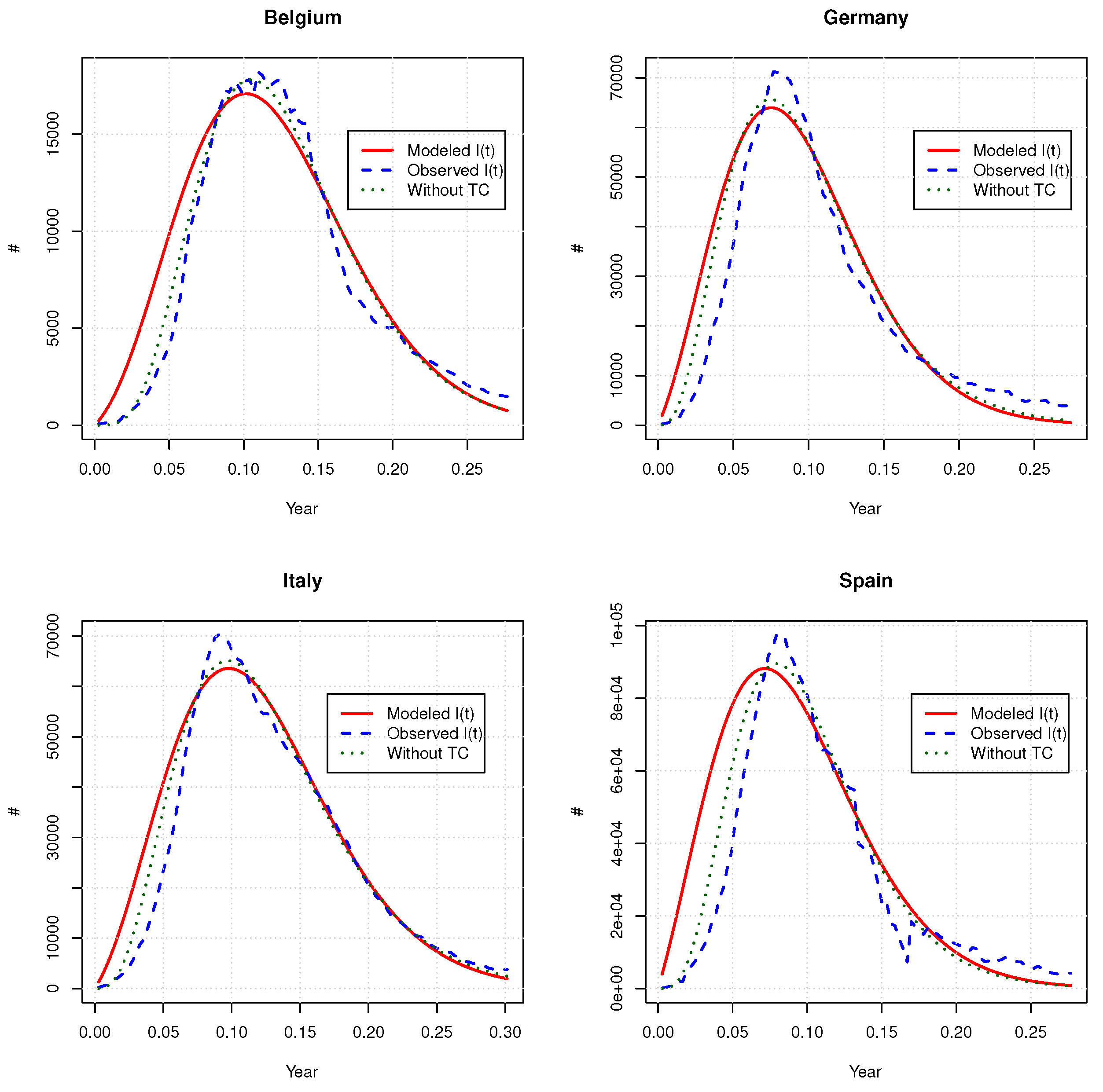
Figure 3 compares the expected number of infectious obtained with the time-changed model and its deterministic counterpart. Globally, we do not observe any similarities between parameters of time-changed and deterministic models. The goodness of fit, measured by the SSE, is also worse for the time-changed version than for the deterministic one. The time change does not fit the right tail of the
curve better and overestimates, on average, the number of infected individuals at the beginning of the pandemic.
Table 7 shows the fair premium rates for the healthcare and death insurances valued in
Section 5. Since the time-changed model predicts on average higher healthcare benefits during the growing phase of the outbreak, the healthcare insurance is slightly more expensive than the one valued with the deterministic model. The death benefits and death insurance premium rates are comparable in both models.
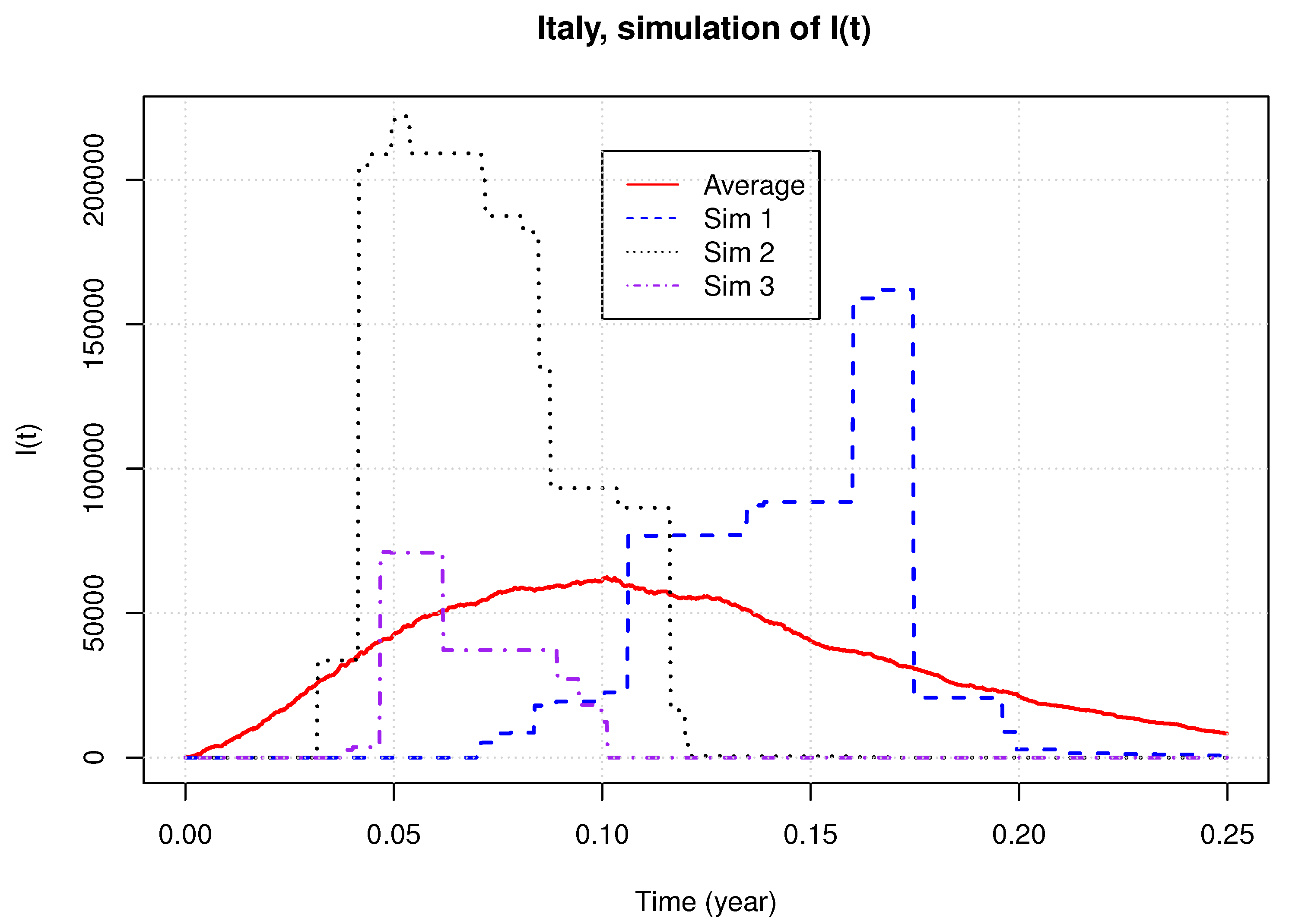
If we limit our analysis to a comparison of the expected number of infected individuals and premium rates, we have the impression that both deterministic and time-changed models are quite similar. However, this is far from being the case, given that the second one is stochastic. In order to emphasize the different behavior of this model, we simulate 2000 samples paths with parameter estimates obtained for Italy.
Figure 4 shows three of these paths and the average over the 2000 simulations. We see that the time-changed model generates curves of
with a different shape than the average sample path. The simulated peaks of the epidemic may be far above the observed one and the timing of this peak displays a high variance. The sample paths are also much more discontinuous than the real evolution of
.
It is also interesting to look at the distribution of the cumulated number of deaths.
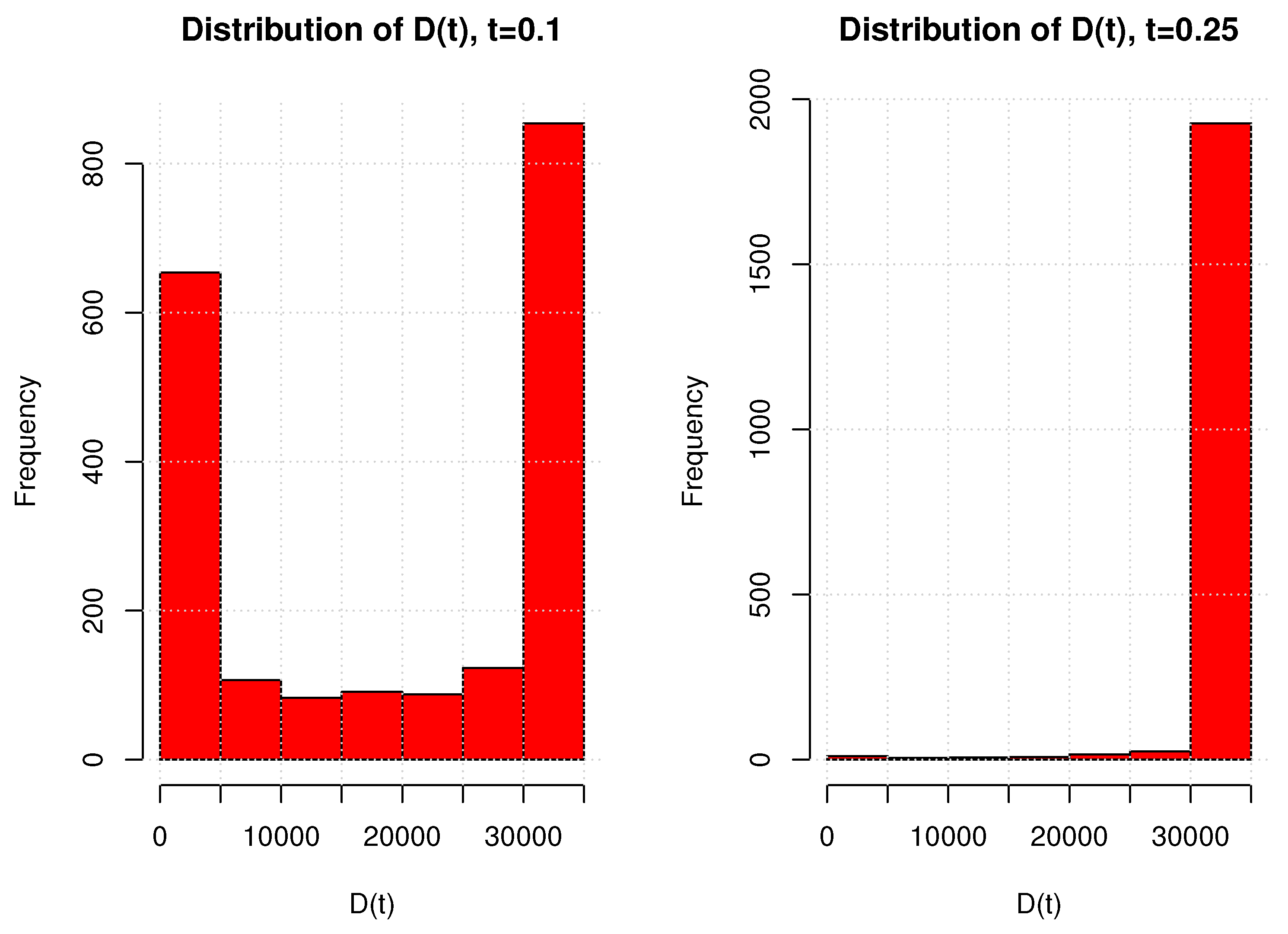
Figure 5 presents the histograms of
for 2000 simulations at time
and
. For
, we have a bimodal distribution, whereas the number of cumulated deaths after a quarter is nearly deterministic. This is explained by the type of randomness driving the model. The stochastic clock either delays or advances the time of the epidemic peak, but it does not modify the ultimate total number of deaths caused by the pandemic.
Table 8 reports the expectations, standard deviations, 5% and 95% percentiles of
, computed by simulations for the other countries. We draw from those figures the same conclusions. The discontinuities of
and the bimodal behavior of
being unlikely in practice (at least for COVID-19), we investigate in the next section, an alternative stochastic extension of the deterministic model.
9. A Jump Diffusion Model
This section presents an alternative stochastic model for the dynamic of the infected population that includes random noise and local resurgence of the epidemic. This model also has an excellent analytical tractability and is estimated by a peak over threshold approach. We consider a probability space
on which a Brownian motion
and a compound jump process
are defined. We denote by
a Poisson process with intensity
, and by
i.i.d. random variables defined on
with a probability density function denoted by
. The expectation and variance of a jump are denoted by
and
, respectively. The compound Poisson process
is defined as the sum of jumps
up to time
t:
We assume that the dynamics of the population of infected individuals is ruled by the following geometric jump diffusion:
where
,
,
are the recovery, mortality and contagion rates, respectively. The term
, with
, is a Gaussian noise, whereas
introduces random discontinuities caused by the discovery of clusters of infection. The next proposition presents the solution of Equation (
32). Under the assumption that
is ruled by Equation (
32), the size of the population of infected people is equal to:
This result is a direct consequence of Itô’s lemma for jump diffusion. In order to evaluate an insurance plan, we need to adopt a dynamic for the cumulated number of deaths,
. As in previous models, we assume that the instantaneous number of death at time
t is a proportion
of the population of sick persons. The differential equation ruling
, the population of susceptible individuals, guarantees that the total size of the population remains equal to
:
The number of deaths is , whereas . Of course, we could include a random noise in the dynamics of , but this would not fundamentally modify the results developed in the remainder of this section. The next proposition presents the first two moments of .
Proposition 5. The expectation and variance of the number of infected persons at time t are respectively equal toand Proof. Given that
is independent from
, the expectation of
is equal to a product of expectations:
As
) is normal,
. The moment-generating function of
is
and
is independent for
. Therefore, we conclude that the expectation of the product of jumps is:
Combining these elements leads to Equation (
35). In a similar manner, we calculate the second order moment of
—that is,
Since
is log-normal,
and
. Furthermore, the expectation of the square of the product of jumps is equal to:
We obtain, then, the second moment of
and the variance in (
36). □
The next proposition presents an analytical formula to evaluate expected healthcare benefits paid up to time t. This result is similar to the one for the deterministic model, except that it takes into account the frequency and the average size of jumps.
Proposition 6. Let us consider a discount rate . The integral of expected discounted numbers of infected is equal to:where and is the gamma lower incomplete function. The proof is similar to the one of Proposition 1. We insert the expression (
34) of
in the integral and obtain Equation (
37). Contrary to the time-changed model, the expected number of deaths and its discounted integral admit closed-form expressions in terms of incomplete lower gamma functions.
Corollary 2. The expected cumulated number of deaths caused by the epidemic at time is equal to If , the expectation of the integral of discounted variation of is equal to: Let us again consider the insurance plan introduced in Equation (4) with a maturity T. The premium rate is still denoted as p. The rate of healthcare expenses is b and the lump sum benefit in case of death is c. The next proposition presents the fair premium rate that ensures the equilibrium of this plan under the assumption that the pricing and real measures are identical.
Proposition 7. For the benefit rates , the fair premium rate that guarantees the actuarial equilibrium of the plan is given by:where the denominator is equal to: Proof. The fair premium rate in a stochastic framework is given by Equation (
28). The integral
is provided by Equation (
37). As
, we infer that
where
admits the following integral representation:
Given that
, the double integral in this last expression becomes:
Therefore, the integral of the discounted expected number of deaths is equal to:
Combining expressions (
42) and (
43) leads to Equation (
41). □
10. Reinsurance in the Jump Diffusion Model
As in the time-changed model, we can evaluate various reinsurance coverages by Monte Carlo simulations. When jumps are constant and equal to
, reinsurance treaties with a payoff dependent on
can be valued with a closed-form expression. In this case, conditionally to
jumps,
is log-normal:
where
. The mean and variance of
are respectively equal to
The following proposition provides an analytical expression for a reinsurance treaty that plans the payment of an amount at time t, where , if . Model parameters are assumed to be the same under the pricing and real measures.
Proposition 8. The value of an excess-of-loss reinsurance covering an excessive number of infected is equal to:whereand is the cumulative probability distribution of a standard normal random variable. Proof. We can rewrite the price of this treaty as a sum of conditional expectations with respect to
:
The conditional expectations may be developed as the difference of two integrals:
The second term, after a change of variable, is equal to:
where
. In the same manner, the first term of Equation (
47) becomes:
and we retrieve the result. □
By construction, the cumulated number of deaths up to time t is proportional to the integral of . Unfortunately, the statistical distribution of is unknown and, therefore, reinsurance treaties covering excess of mortality must be valued by simulations.
11. Estimation of the Jump Diffusion Model
The jump diffusion model is fitted in two steps. Let us recall that
where
and
are the observation times for
. The first step consists in estimating
,
and
by minimizing the weighted sum of squares between the expected and observed numbers of infected persons:
Given that the expectation of
in the jump diffusion approach coincides with the deterministic model, we obtain the same estimates
,
as those in
Table 2. In the second stage, we fit the jump process by the peak over threshold method. From Equations (
33) and (
35), we define
as the ratio of the process
on its expectation:
Using Itô’s lemma, we infer that
is driven by the following infinitesimal dynamics:
The value of
at time
is noted
and we define
the discrete approximation of
. If the time lag of one day between two successive observations is noted
, according to Equation (
49),
is approximately the sum
where
and
. A jump is believed to occur when
is above a threshold, noted by
, where
q is a confidence level. To define the threshold, we fit a pure Gaussian process to the time series of
. The unbiased estimators of
and
are:
If
denotes the cumulative distribution function of a standard normal,
is set to the
q percentile of the Gaussian process:
. The time
of the
jump is therefore:
and the sample path of
is approached by the following time series:
Under the assumption that the diffusion is negligible with respect to jumps, we assimilate to when a jump is detected at time .
We have applied this estimation procedure to COVID-19 data sets for Belgium, Germany, Italy and Spain. The estimates
and
are found by minimization of weighted least squares as shown in Equation (
48). We use the same weights as those used to fit previous models (see Equation (
17)). The other parameters are estimated by the peak over threshold method and are reported in
Table 9. Given that the number of confirmed cases in March is underestimated due to the penury of tests, we mainly focus on the period from mid-April to mid-June to calculate the time series of
. The threshold confidence level is set to 90%.
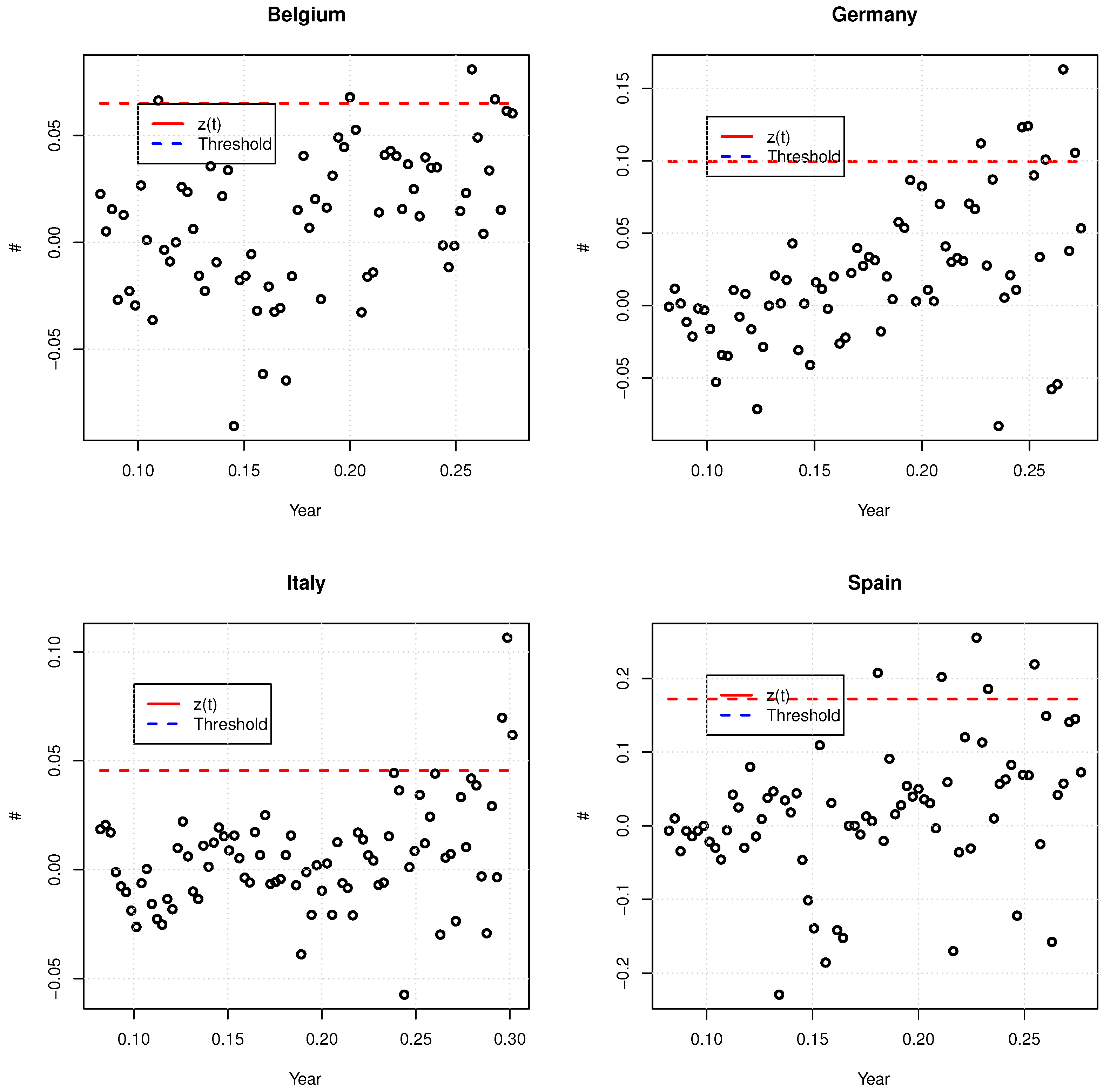
Figure 6 shows those series and the threshold level. For Spain, we have not taken two abnormally high and low values into account due to retrospective adjustments of the number of confirmed cases. For Belgium and Spain, the
values have a mean close to zero and the variance seems more or less constant for different time windows. This confirms that the postulated dynamic in Equation (
50) for
is acceptable for those countries. For Italy, the variance of
seems to raise during the month of June, but their mean is close to zero. For Germany, the
values have a residual linear increasing trend and their variance seems to increase as it does for Italy. The consequence is that the peak-over-threshold method tends to overestimate the size and frequency of jumps. Nevertheless, this is a conservative approach from the insurer point of view and, therefore, we accept these parameter estimates. For the same reason, we do not consider negative jumps.
By construction, the expectation of the jump diffusion model corresponds to the deterministic model of
Section 3. Therefore, the fair premium rate of an insurance plan covering healthcare expenses and death benefits are the same with both approaches. We refer the reader to the previous
Section 5 for numerical examples. However, the jump diffusion model can generate a wide variety of sample paths for
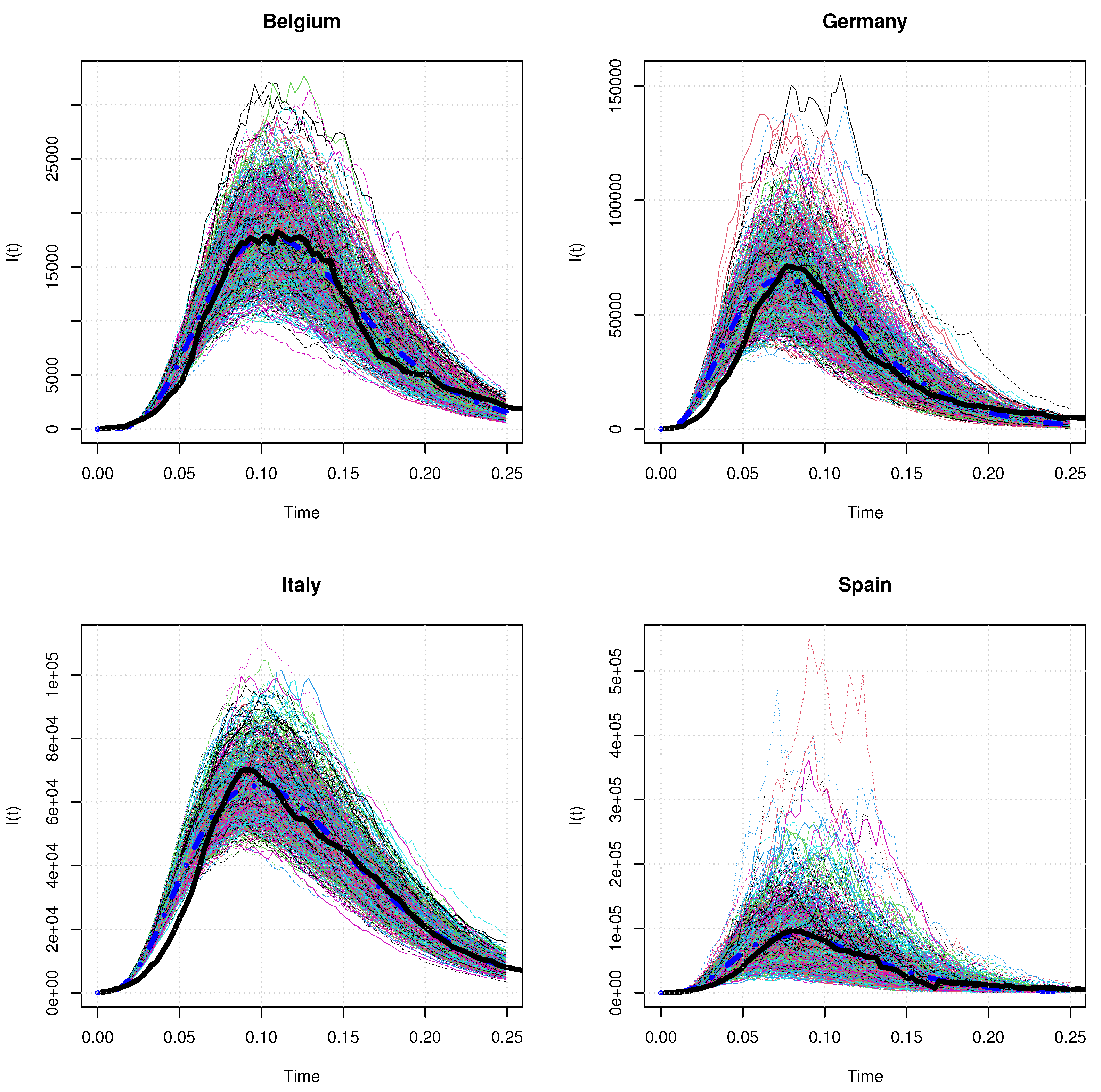
. This point is illustrated in
Figure 7 that shows 1000 simulated paths and the expectation of
over a quarter. Notice that these simulations are performed with the assumption that jumps
J are constant and equal to
.
Contrary to the time-changed approach, the jump diffusion model generates smoother sample paths which all appear as likely scenarios for the evolution of the infected population. These graphs also display the expected and the observed number of infected cases for each country. It reveals that the real sample path of
for each country is a likely realization of the jump diffusion model, at least for
. At the beginning of the pandemic, the real sample path of
bounds from below simulated trajectories. This is a direct consequence of choices made in
Section 5 for calibrating the average trend of the model. At the start of the epidemic, testing polices were in the process of being deployed and the number of infected cases was probably underestimated. This motivates our choice of underweighting observations collected in the early ascending phase. We also remark that the peak of infected cases is significantly higher than the observed one in some scenarios. To illustrate this,
Table 10 reports the 90% and 95% percentiles of the simulated maximum of infected cases. The ratios of these 95% percentiles on real numbers of infected cases at the epidemic peak range from 121.23% for Italy up to 202.49% for Spain.
Table 11 reports statistics about the simulated number of deceases over one quarter. Globally, the mean and standard deviation of
seems credible and the distribution of
does not display any bimodality as in the time-changed model.
Table 12 presents the prices of a few excess-of-loss reinsurances with
and
as underlying risks. The treaties on
have a threshold
K equal to one-fourth of the total number of reported cases over the considered period of time (see
Table 1). The time horizon of the contract and the capital by unit in excess are set to
year and
, respectively. Prices are calculated with the closed-form expression (
46). We use Monte Carlo simulations for the valuation of reinsurance contracts covering an excessive mortality. The threshold
K is set to the observed number of deaths observed over the considered period (see
Table 1). The time horizon and the capital by unit in excess are respectively set to
year and
.
12. Conclusions
The valuation of actuarial commitments requires us to integrate over time the size of infectious and susceptible populations. Since existing compartment models do not admit closed-form expressions for these quantities, actuarial calculations are in this framework computationally intensive and subject to numerical errors. The three models proposed in this article remedy to this issue and present a high degree of analytical tractability.
The first model is purely deterministic. The basic reproduction number, , decays with time in order to replicate the impact of preventive measures to curb the epidemic. Contrary to the SIR, the empirical tests performed on COVID-19 data confirm that the model explains the first wave of such an epidemic. Furthermore, the insurance premium rate admits a closed-form expression within this framework. The main disadvantage of this approach is the absence of random effects that prevents to evaluate the incurred extreme costs.
The second model is a time-changed extension of the deterministic one. The time of the pandemic peak is randomized by observing the process on a stochastic time scale. The main advantage of this approach is that it preserves the main features of the deterministic model and leads to comparable premium rates. Nevertheless, the simulation study reveals that simulated scenarios display a different trend from what is observed for the COVID-19 outbreak. Furthermore, the stochastic clock modulates the speed at which the pandemic evolves but do not modify the sizes of infected and susceptible populations.
This article proposes a second stochastic extension of the deterministic model based on a jump diffusion process. In this approach, the rate at which patients cease to be considered as infected is noised by a Brownian motion. This allows us to randomize the duration of illness. The apparition of local clusters of infected causing a sudden increase of the number of contagious cases is replicated by the jump component. This model presents several interesting features. As it behaves, on average, as the deterministic approach does, it keeps a high analytical tractability for actuarial applications. On the other hand, the model is able to generate realistic noised sample paths of infected cases. This feature allows us to price reinsurance contracts, such as excess of loss treaties, that cannot be valued in a deterministic framework. Last but not least, it is remarkably easy to estimate its parameters with the proposed “peak-over-threshold” method.
Notice that, by construction, the contagion rate per capita decreases as , the size of the infected population, converges to zero after having reached the epidemic peak. In a similar way to the SIR model, the solutions proposed in this article are then designed for explaining a single epidemic wave with, eventually, random recovery duration and discovery of local clusters of infected individuals.
This observations opens the way to further research. Instead of a deterministic starting date for the epidemic, we can replace it by the jump time of a self-exciting point process, e.g.,
Hainaut and Moraux (
2019). In its simplest version, the intensity of this process is persistent and suddenly increases as soon as a jump occurs. Within this approach, the starting date of the pandemic becomes random and the probability of observing a new epidemic wave raises after the first one but decay exponentially to its baseline level. Other possible extensions consist to randomize the mortality rates or to develop a compartmental version with subpopulations of infected individuals.
