The Sustainability Factor: How Much Do Pension Expenditures Improve in Spain?

Abstract

The reform of 2013 represented a qualitative leap in the reform of the Spanish pension system. Unlike its predecessors, it introduced two automatic resetting mechanisms similar to those of other European countries. The first is the sustainability factor, scheduled to come into effect in 2019 but delayed until 2023, and its ultimate reversal cannot be ruled out. The objective of this study was to quantify the savings, or the lowest expenditure, that can be achieved in the Spanish public contributory pension system by applying it. These savings are measured in terms of cash—of annual expenditure—and in terms of accrual by calculating its present actuarial value. Combining these two methods is one of the contributions of this work. This work was only intended to analyze the impact of the Sustainability Factor, therefore, it did not take into account the impact of the Pension Revaluation Index, which is the second mechanism introduced in the reform of the pension to 2013. An ad hoc projection method was used, combining microdata from the Continuous Sample of Working Lives (MCVL), aggregate data from the pension system, the financial-actuarial projection method, and actuarial techniques. The diversity of the data used is the second contribution of this work. The application of the sustainability factor would improve the viability of the system, since the savings that could be achieved, measured in terms of GDP for each year, would be 1.029% by 2050; 1.094% in 2057, the maximum; and 1.026% in the last year of projection. In terms of the present actuarial value and as a function of annual GDP, in 2050, the savings would be 1.27%, 1.40% in 2044, the maximum, and in 2067 it would decrease to 0.98%.

1. Introduction

There has been pressing concern regarding the sustainability of public pension systems in Europe for decades. Part of this stems from demographic ageing, caused fundamentally by the continuously increasing life expectancy of the population1. In addition, the deep financial and economic crisis that began in 2008 exacerbated the financial difficulties of public pension systems and accelerated their reform. The economic effects of the COVID-19 pandemic will undoubtedly contribute to the complication of these difficulties.

Most of the reforms implementing pay-as-you-go systems2 have been parametric, with adjustments in the basic data of the system, such as an increase in the legal retirement age and the number of years taken into account for calculating the starting pension or tightening the conditions for being granted early retirement3.

Among the parametric changes, two types must be distinguished:

(a)

Those that have adopted a rigid system, since they have changed the starting parameters to other fixed values, although these changes happen over long transitional periods.

(b)

Those that have adopted a flexible system, since the values of the parameters depend on some reference or variable external to the system. These are called automatic resetting mechanisms.

In this paper, we address the Sustainability Factor, which is one of the two automatic adjustment mechanisms that were approved in Spain in 2013, although its design comes from the 2011 reform.

Furthermore, between the two major pension reforms 2011 and 2013, another minor regulatory change was approved through (Royal Decree-Law 5 2013). This regulation introduced several modifications that fundamentally affected the area of early retirement, considering that the measures previously approved in the 2011 reform did not allow stopping the early abandonment of working life and, consequently, they were insufficient to bring the effective retirement age closer to the legal age. The changes introduced to toughen early retirement consisted in raising the minimum access age, increasing penalties, and reducing the amount of the maximum pension which workers with access to this type of retirement are entitled to.

The current work is structured as follows. In the second section, the main features of the automatic adjustment mechanisms are discussed. The third section explains the SF that was adopted in Spain in 2013. The following section shows the financial-actuarial projection model with microdata that we used. Next, a base scenario is presented, and the savings in pension expenditures are shown after the application of the SF both in terms of cash and in terms of present actuarial value. After that, a sensitivity analysis is performed, modifying some of the variables that were used, and the effect of the delay in its application is also studied. The work ends with conclusions and bibliographic references.

2. Automatic Adjustment Mechanisms

According to Gaya et al. (2013), parametric reforms refer to “any mechanism that automatically reviews any of the fundamental parameters of the pension system based on the evolution of some external variable that affects its sustainability, whether it is of a demographic, which is the most common, or of an economic nature”. Consequently, as noted by Devesa et al. (2016) “the design of any sustainability factor involves defining, on the one hand, the external variable that will be taken as a reference, that is, the variable the system adjustments will depend on; and, on the other hand, defining the internal variable or parameter of the system the adjustment will fall on”.

One of the most important characteristics of the pension reforms carried out in the last two decades is that many countries have chosen to introduce some type of automatic resetting mechanism. Some of them did so in the late 1990s and the early 21st century, but the vast majority were implemented by the end of 2010 in response to the sustainability problems generated by the 2008 economic crisis. These types of mechanisms are part of the set of measures recommended by the European Commission (2012) to the different member states to reduce future spending on pensions.

Table 1. EU countries with automatic resetting mechanisms.

Country	Automatic Balancing Mechanism	Pension Amount Linked to Life Expectancy	Legal Retirement Age Linked to Life Expectancy	Introduction Year of the Automatic Resetting Mechanism
Italy		X	X	1995 and 2010
Latvia		X		1996
Sweden	X	X		1998 and 2001
Poland		X		1999
France		X		2003
Germany	X			2004
Finland		X	X	2005 and 2015
Portugal		X	X	2007 and 2013
Greece			X	2010
Denmark			X	2011
Spain	X	X		2011 and 2013
The Netherlands			X	2012
Cyprus			X	2012
Slovakia			X	2012
Lithuania	X			2016
Estonia			X	2018

Note: In Malta, the Social Security Law obliges the government to present a report every five years in Parliament on the financial status of the pension system and to propose recommendations to ensure that a stable proportion is maintained between contribution periods and time periods during which it is expected that the pension will be paid. Source: Economic Policy Committee and Social Protection Committee from the European Commission (2020).

show that more than half of the EU countries have implemented at least one automatic resetting mechanism. The most common case is for the regular retirement age to be related to the evolution of life expectancy, with the aim of taking a more dynamic approach toward the age at which people can retire. Thus, individuals who belong to different generations and therefore have different life expectancies can receive their pension over the same time frame4.

3. The Sustainability Factor of the Spanish Pension System

The Spanish pension system currently has two automatic resetting mechanisms. Both were introduced in the 2013 pension reform (Law 23 2013):

(a)

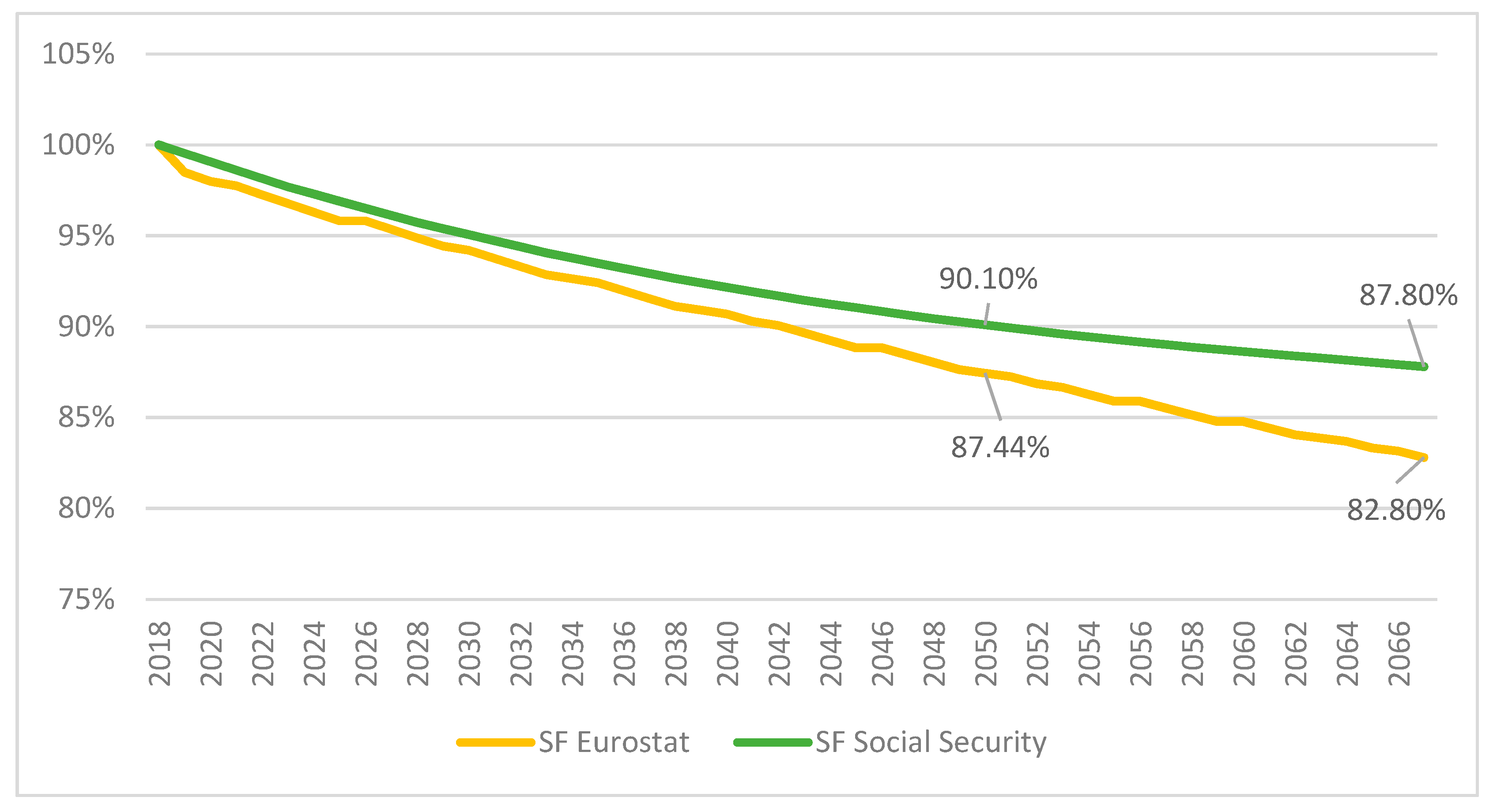
The sustainability factor (SF) modifies the starting amount of the retirement pension benefit as life expectancy changes5.

(b)

The pension revaluation index adjusts the revaluation of all pensions based on the financial health of the system.

Several studies on SFs have been published (Gaya et al. 2013; Sanchez Martin 2014; Hoyo 2014; Pérez Alonso 2016; Díaz-Giménez and Díaz-Saavedra 2017; Alda et al. 2018), including on its design, advantages, and disadvantages. However, there are few evaluations of the impact of the SF on savings in pension expenditures6. The contributions of our study are that it not only assesses the effect of the SF on pension expenditure but also creates a model to estimate this expenditure based on the information available. A financial-actuarial method that uses microdata along with aggregated social security data to fit the hypotheses was applied. This method, although it has been designed for Spain, could be applied to any country since it adapts to the available information.

Given the large number of specificities of all pension systems, financial models are strengthened when actuarial elements are added. These elements take into account longevity, which is fundamental in the field of pensions. In Spain, we have both aggregated data and microdata from the Continuous Sample of Working Lives; in our case, we used the data from 2018 (hereinafter MCVL2018)7, though the model we applied allows the joint use of both data sources. Unlike other studies, this one focusses only on the retirement pension.

As indicated above, the SF is one of the two automatic resetting mechanisms that were introduced in Spain in the 2011 pension reform. It was refined in the 2013 pension reform, which defines it as “an instrument that automatically adjusts the amount of the starting retirement pension to the evolving life expectancy, at 67 years, of the pensioner population”. That is, in Spain, it was decided that the SF adjustment would fall on the starting amount of the retirement pension and not on the retirement age, as happens in many European countries8.

The fundamental objective for which this instrument was designed was to improve the intergenerational equity of the Spanish pension system9 because it adjusts the starting pension of new retirees. Thus, two individuals who have similar careers and who retire at the same age will receive the same total pension amount, regardless of their retirement date. Therefore, in reality, the SF is not an element of sustainability—as its name indicates—but of actuarial equity, though as life expectancy increases, the result of the adjustment, ceteris paribus, will be a lower starting pension than in the absence of SF. This will generate a decrease in pension expenditure and an improvement in system sustainability. It will also cause the internal rate of return (IRR) of the pension system to be maintained since, as we have mentioned, the starting pension is adjusted exactly to compensate for the increase in life expectancy. Therefore, estimating the impact of the SF on pension spending was one of the objectives of this study.

Another parameter is added to the SF, in addition to the ones already present in the formula for calculating the starting pension (regulatory base, coefficient by contribution years, and by retirement age) to safeguard the system against longevity risk.

Initially, the effective implementation of the SF formula was planned for 2019 but has been delayed until 2023, and its reversal has not been ruled out. Therefore, this study will consider options regarding the reversal of the SF and the effect this would have on the system.

The specific formula, designed in Law 23 2013, for the calculation of the SF, starts with the following relationship, where for each period, the 5-year variation of the ratio between the life expectancies of individuals at age 67 is annualized:

$$\mathrm{Period} \left[2019, 2023\right]:{ \mathrm{e}}_{67}^{*\left[2019,2023\right]}= {\left(\frac{{\mathrm{e}}_{67}^{2012}}{{\mathrm{e}}_{67}^{2017}}\right)}^{\frac{1}{5}}$$

$$\mathrm{Period} \left[2024, 2028\right]:{ \mathrm{e}}_{67}^{*\left[2024,2028\right]}= {\left(\frac{{\mathrm{e}}_{67}^{2017}}{{\mathrm{e}}_{67}^{2022}}\right)}^{\frac{1}{5}} \dots$$

The SF of any year t is calculated by multiplying the SF of the previous year by the coefficient e^* corresponding to the 5-year period of the calculation year:

$${\mathrm{SF}}^{\mathrm{t}}={\mathrm{SF}}^{\mathrm{t}-1}{ \mathrm{e}}_{67}^{*\left[\mathsf{\tau },\mathsf{\tau }+4\right]};\mathrm{such} \mathrm{that} \mathrm{t} \mathrm{is} \mathrm{an} \mathrm{integer} ϵ\left[\mathsf{\tau },\mathsf{\tau }+4\right]$$

where ${\mathrm{e}}_{67}^{\mathrm{t}}$ is the life expectancy of a 67-year-old in year t. SF^t is the sustainability factor in year t. ${\mathrm{e}}_{67}^{*\left[\mathsf{\tau },\mathsf{\tau }+4\right]}$ is the life expectancy average annual change at 67 from the previous 5-year period [τ, τ + 4].

4. Financial-Actuarial Model with Microdata to Simulate Retirement Pension Expenditures

From an aggregate perspective, pension expenditure, expressed in relation to GDP, depends on three types of factors (Hernández de Cos et al. 2017)—demographics, the labour market, and the ratio between average pension and productivity, which can be reduced to the ratio between the number of pensions multiplied by the average pension in relation to GDP. Therefore, the formula for estimating the pension-expenditure-to-GDP ratio would be

$$\frac{\mathrm{PE}}{\mathrm{GDP}}=\frac{\mathrm{NP}}{\mathrm{Pop}}\frac{\mathrm{Pop}}{\mathrm{L}}\frac{\mathrm{AP}}{\mathrm{W}}\frac{\mathrm{W}\ast \mathrm{L}}{\mathrm{GDP}}=\frac{\mathrm{NP}\ast \mathrm{AP}}{\mathrm{GDP}}$$

(1)

where PE is the pension expenditure; GDP is the gross domestic product; NP is the number of pensions; AP is the average pension; Pop is the population with age of work; L is population working; W is the wage.

The average pension and the number of pensions will be estimated from multiple perspectives, since information from both the aggregated statistics and the microdata provided by the MCVL will be used.

First, the pension expenditure for retirement benefits must be obtained for the year 2019 (the notation used is shown in Scheme 1).

New retirement pension expenditures (year 2019):

Σ No. N¹⁹ ˑ AP¹⁹ ˑ SF¹⁹.

In the first year of analysis, 2019, pension expenditure in the case where the SF is applied will be the product of the number of new registrations (new pensions) for 2019, multiplied by their average pension benefit of that year and by the SF corresponding to 2019. Savings in 2019 pension expenditures will be calculated by comparing this result with what would be obtained if the SF were not applied, that is, when the SF equals 1.

Retirement pension expenditures (year 2020):

Σ No. N²⁰ ˑ AP²⁰ ˑ SF²⁰ + Σ No. N¹⁹ ˑ AP¹⁹ ˑ SF¹⁹ ˑ ₁pxj¹⁹ (1 + α).

In the second year of analysis, 2020, pension expenditure is calculated as the sum of two sums. The first sum is equivalent to that calculated in the first year, but adjusted to 2020 values. The second sum includes the expenditure corresponding to the surviving cohort who retired in 2019 (therefore multiplied by the probability of survival) adjusted by the estimated pension revaluation index, α.

Retirement pension expenditures (year 2019 + s):

In any given year, s years after the start of the calculations, 2019 + s, we will obtain

Σ No. N^{19 + s} · AP^{19 + s} · SF^{19 + s} + Σ No. N^{19 + s − 1} · AP^{19 + s − 1} · SF^{19 + s − 1} · ₁p_xj^{19 + s − 1} · (1 + α)
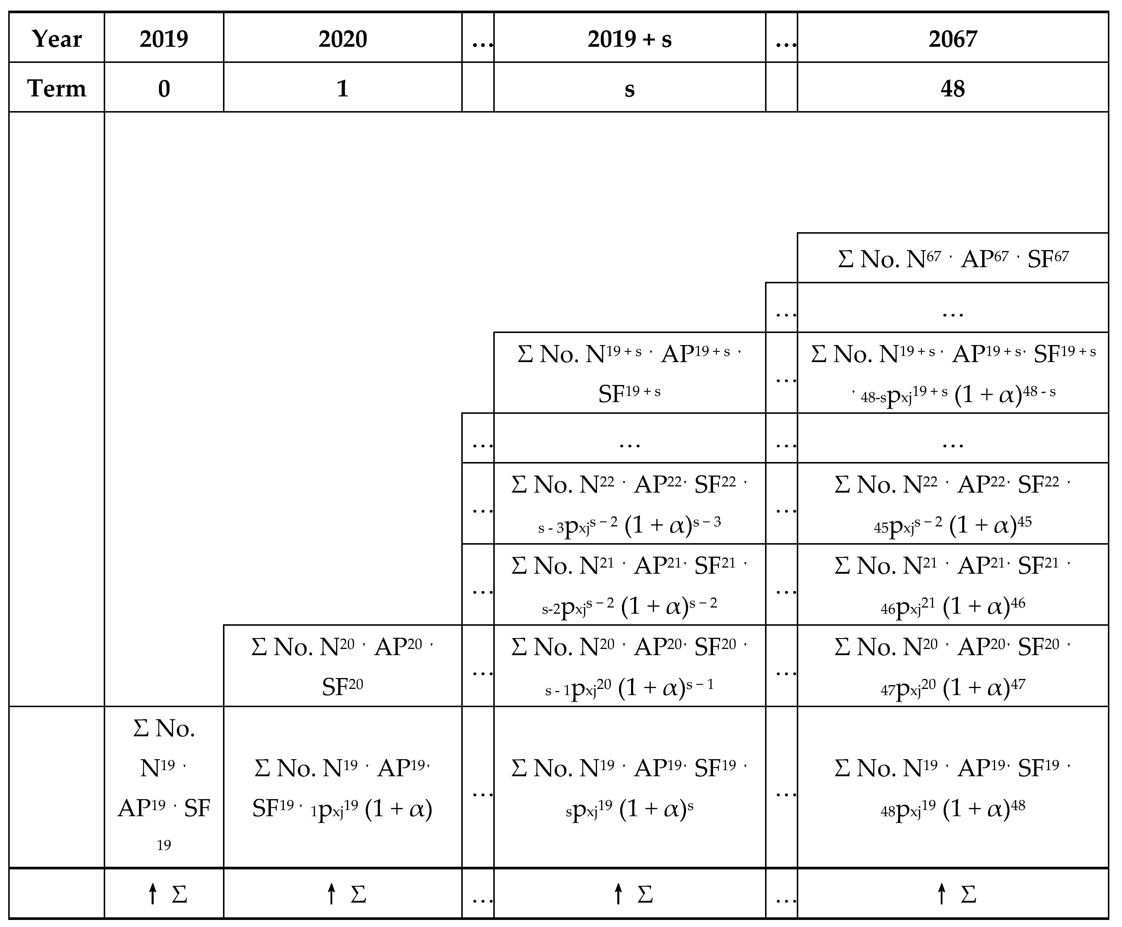
+...+ Σ No. N²⁰ · AP²⁰ · SF²⁰ · _s−1p_xj²⁰ · (1 + α)^{s − 1} + Σ No. N¹⁹ · AP¹⁹ · SF¹⁹ · _sp_xj¹⁹ · (1 + α)^s.

In the year 2019 + s, retirement pension expenditure is the sum of s + 1 components. The first sum is equivalent to that calculated in the first year, but adjusted to 2019 + s values. The second sum includes the expenditure corresponding to the surviving cohort who retired the previous year, in 2019 + s − 1, adjusted by the pension revaluation index α. The penultimate corresponds to the surviving 2020 cohort of retirees and the last to the surviving 2019 cohort, in all cases adjusted for the corresponding estimated revaluation index.

Scheme 1 shows the procedure followed to calculate the pension expenditure.

In this study, we worked with two models of expenditure measurement, one in terms of cash and the other in terms of accrual.

-

In terms of cash, although this is the model that has been used by multiple researchers10, we intended to improve upon it by introducing both aggregate and microdata information. We did this because of the different levels of information that we can extract from each of these bases.

-

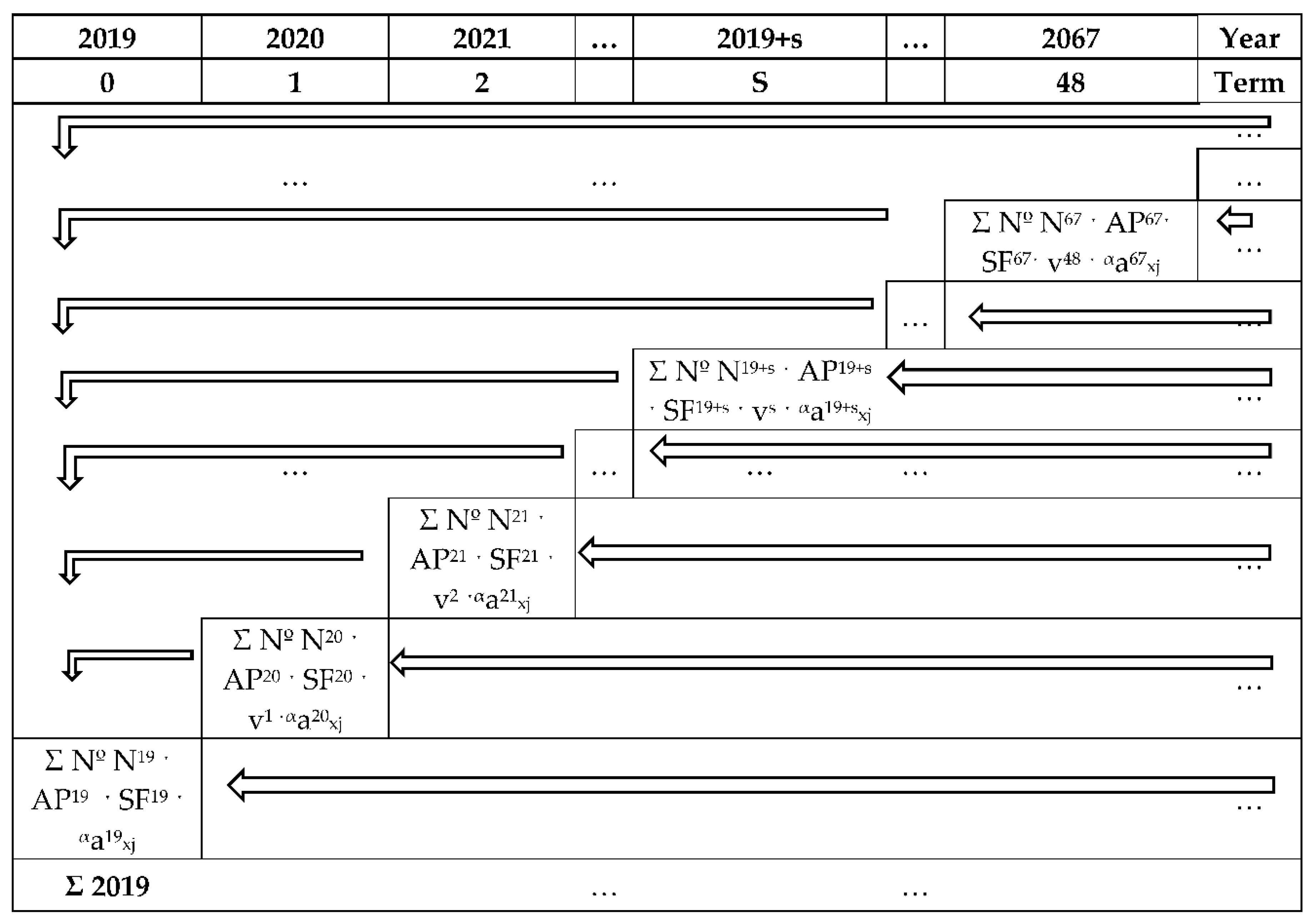
The accrual model, which requires the calculation of the present actuarial value of pension expenditure, gives us a complementary view of the information on the cash balance. The box model does not collect information on everything that will happen with each cohort but rather what happens each year. Analyzing expenditure from the actuarial point of view involves

• Having a global perspective of what happens with a cohort or group of individuals during the entire contributory period.
• Knowing the effect on the increase in the implicit debt of the pension system due to not applying the SF.
• Knowing the amount that would have to be allocated annually to meet the new commitments arising from not applying the SF.

By “present actuarial value”, we mean the actuarial sum of the expenditure generated for each group of individuals who retire in a given year, that is, the value of future flows updated by a financial factor (which takes into account different availability over time) and by a statistical factor (to adjust for the probability of survival).

As seen in Scheme 2, each year, this method takes into account not only the cash expenditure of that same year but also the present actuarial value of all expenditure flows for that cohort. The formulas used are as follows (the notation used is shown in Scheme 2):

PAV Retirement pension expenditures (2019 cohort):

Σ N° N¹⁹ · AP¹⁹ · SF¹⁹ · ^αa¹⁹_xj

In the first year of analysis, 2019, the present actuarial value of pension expenditure in the case of applying the SF will be the product of the number of new pensions for 2019, their average benefit amount in 2019, the SF corresponding to 2019, and the present value of an annuity that grows in a geometric progression of ratio α.

PAV Retirement pension expenditures (2020 cohort):

Σ No. N²⁰ · AP²⁰ · SF²⁰ · ^αa²⁰_xj · v¹

In the second year of analysis, 2020, the present actuarial value of pension expenditure is obtained in a similar way as in the previous year. The number of new pensions in 2020 will change, as will the average pension benefit of that year, the SF of that same year, and the present value of the annuity changes because, although the average retirement age of all cohorts is the same, the value of the income changes since the mortality tables used are dynamic, implying that the probabilities vary by year. In addition, this present actuarial value is multiplied by the factor v¹ = (1 + i)⁻¹ to update it financially11 until 2019. By taking the difference from the scenario where the SF equals 1, we obtain the savings in total expenditures:

PAV Retirement pension expenditures (2019 + s cohort):

Σ No. N^{19 + s} · AP^{19 + s} · SF^{19 + s} · ^αa^{19 + s}_xj · v^s

In any given year, s years after the start of the calculations, i.e., year 2019 + s, the scheme is similar to the previous ones, and it would be necessary to update by s years, with the factor v^s = (1 + i)^−s, to evaluate the expenditure in 2019.

The arrows in Scheme 2 indicate that there is a double process to obtain the present actuarial value: first, it is discounted until the beginning of the annuity and then that value is discounted until the time of valuation, which is 2019.

5. Working Hypothesis for the Application of the Financial-Actuarial Model, with Microdata, to Generate Pension Expenditure

A complex projection model of the expenditure of the Spanish retirement pension system has been developed to adjust it to the data available in Spain, but it can be valid for any other country since it allows adaptation to existing information. It could be classified as a financial-actuarial model with microdata and adjusted to the aggregate data of the system. The model is structured by combining different instruments:

✓

Instrument 1. Microdata: Microdata were used, obtained from the MCVL2018, with which it was possible to generate information on the distribution of both the new retirement pensions and the total number of retirement pensions. This allows us to know, for each age and gender, the number of pensions and amount of their benefits, which is essential to apply the actuarial methods.

✓

Instrument 2. Aggregate data: Real aggregate data on the total number and average amount of retirement pensions have also been used. This information obtained from Social Security, and the data from the MCVL2018 allow us to obtain the results for the population.

✓

Instrument 3. Actuarial method. An actuarial method has been used, employing financial factors, survival probabilities, and annuities, which are necessary to adequately project the evolution of the different cohorts of retirees, as well as to correctly quantify them.

✓

Instrument 4. Financial method. A financial or arithmetic projection method has been applied, complementing all the information obtained from the previous instruments.

The joint use of the four instruments will allow us to measure the impact of applying the SF or not in terms of the cash value and the present actuarial value of the annual expenditure. These two complementary views enrich the analysis. Apart from errors, this is the first time that such a complete model has been designed not only for Spain but for other countries in our environment. The idea underlying our model is to bring together different methods and different information to achieve a more elaborate projection than that of the models that rely on a single technique.

The model consists of several components whose aggregation will allow us to project expenditures on contributory retirement pensions. In this section, we will work with a baseline scenario, which, in the section, after that will be subjected to a sensitivity analysis. The methodology and working hypotheses considered are presented below.

5.1. Projection of the Number of New Retirement Pensions in the Period 2018–2067

From the MCVL2018, (Spanish Continuous Sample of Working Lives 2018), the distribution by gender and age in 2018 of the number of new retirement pensions has been obtained12 (

Table 2. Average data on new retirement pensions in 2018.

Variable	All	Men	Women	% Men	% Women	Men/Women
Number	12,245	7014	5231	57.28%	42.72%	1.341
Average retirement age	64.44	64.24	64.80	99.69%	100.56%	0.991
Average annual amount	18,562	20,491	15,976	110.39%	86.07%	1.283

Source: Own elaboration based on the MCVL2018.

).

To determine the number of new retirement pensions registered (key to calculating the SF), in the period 2018-206713, the following iterative procedure was followed.

1st

The number is based on the variation of the number of pensions provided by the Social Security estimates until 2050. For the years 2051 to 2067, it has been assumed that the average variation will stay between the 2045 value and the 2050 value. These data were adjusted according to the growth in the number of retirement pensions between 2016 and 2019, which is 50% higher than the total pensions: 1.76% for retirement compared to 1.17%. In addition, within retirement, they were adjusted again by gender to keep growth between the 2016 and 2019 levels, which is 1.08% for men and 3.01% for women.

2nd

The distribution by age and gender of the total existing retirement pensions in the year 2018 was obtained from the MCVL2018 regarding the total pensions of the system (

Table 3. Average data on retirement pensions in 2018.

Variable	All	Men	Women	% Men	% Women	Men/Women
Number	240,215	148,599	91,616	61.86%	38.14%	1.62
Average retirement age	73.86	73.89	73.78	100.04%	99.89%	1.002
Average annual amount	15,485	17,858	11,636	115.32%	75.14%	1.53

Source: Own elaboration based on the MCVL2018.

).

3rd

The next step is to apply the survival probabilities by age and gender to the previous distribution. The difference between the number of pensions of survivors from the previous year and the number of pensions estimated in sub–paragraph 1 will give us the number of new pensions that year.

4th

Next, assuming that all the retirement pension withdrawals come from death14, the number of new pensions calculated in sub-paragraph 3 is added to the pensioner group, always maintaining the same age and gender distribution as for the new pensions for 2018. This process is repeated for the next few years.

5.2. Projection of the Starting Retirement Pension Benefit in the Period 2018–2067

Again, we highlight that we analyzed only retirement pensions, without taking into account other coverages. With regard to the amount of the starting pension of new pensioners, the average annualized data provided by Social Security for 2018, which was EUR 18,357.25 were split, a result of multiplying the average monthly benefit of EUR 1,311.23 by the number of payments, which is 14.

The future variation in the average starting benefit of new pensioners has consistently been 1.411% according to Social Security data for the years 2010 to 2018. This variation in the average benefit consists of two elements, which have been obtained from the MCVL2018.

These are the regulatory base, which has increased by 1.78% per year in that period and the theoretical replacement rate (percentage applied to the regulatory base), which has decreased by 0.36% annually.

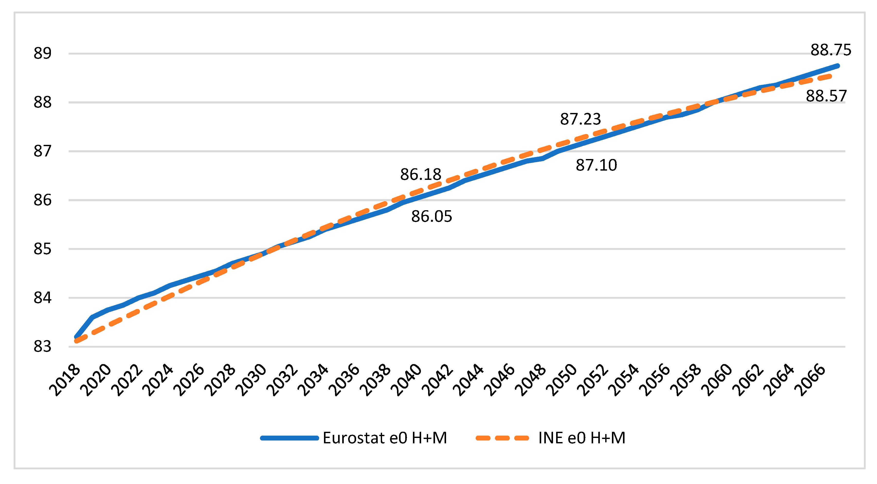
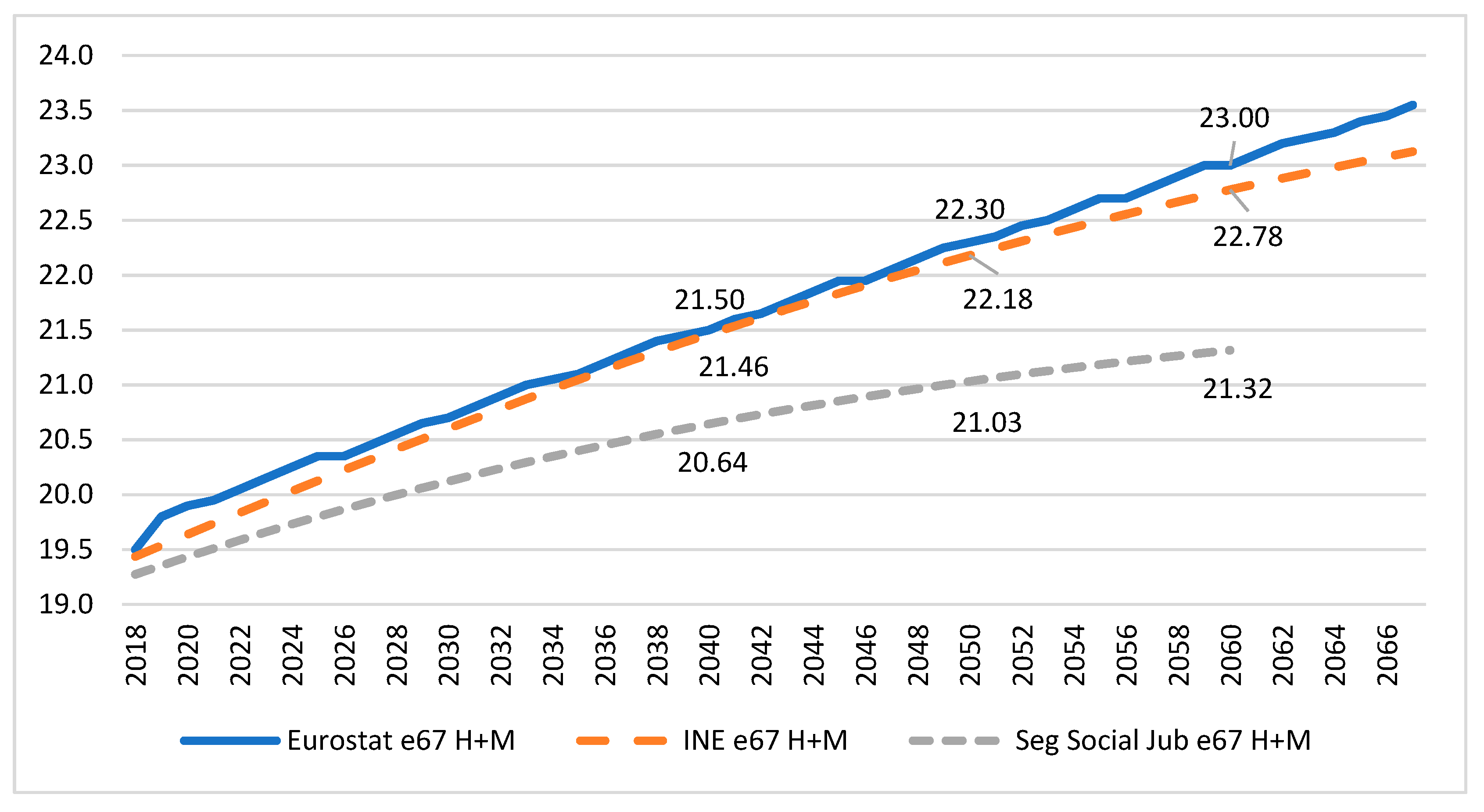
5.3. Mortality Tables

The mortality table is a very important element because it pivots much of the calculation. Three tables were initially used: the INE (National Statistics Institute) projections between 2018 and 2067, by age and sex; the unisex mortality tables for Social Security retirees between 2018 and 2060, by age; and those of Eurostat between 2018 and 2100, by age and gender.

Social Security tables have several drawbacks. On the one hand, they provide data up to 2060, but they have not been updated for many years (the earliest data are from 2007) and have yielded very different results to the other two. In addition, this table does not provide separate data for men and women, and retirement data begin at age 50. However, as seen in Figure 1, in the case of life expectancy at birth (e₀), those of the INE and Eurostat are quite similar, intersecting at several points.

As seen in Figure 2, if the comparison is made between the three mortality tables and with data on life expectancy at 67 years (e₆₇), life expectancy in the Eurostat table is always higher than that of the INE, although not much, but this difference appears to grow after 2055. However, the Social Security data are far off from the other two and, in addition, only go until 2060. For all of the above reasons, the Social Security tables were not analyzed. Given the small difference and the possibility of extending the study to 2100 (in contrast to the INE’s 2067), Eurostat was chosen.

5.4. Sustainability Factor

The SF was applied only once, at the time when the retirement pension was collected. Figure 3 shows the SF values using the Eurostat dynamic tables and taking the annual values15. The SF reaches a value of 87.44% in 2050.

As seen in Figure 4, the social security mortality tables would generate higher SF values, but as we have mentioned above, this may be due to the improved survival compiled in the most updated Eurostat tables.

5.5. Other Working Hypotheses

The rest of the hypotheses adopted in the baseline scenario are shown in

Table 4. Hypotheses adopted for the baseline scenario.

Parameter	Baseline Scenario
Interest rate	2%
Inflation	1.6%
α = Pension revaluation	1.6%
GDP growth since 202116	Ageing Report
β = Variation in the average benefit of new retirement pensions	1.411%
Mortality tables	Eurostat

Source: Prepared by the authors.

. These hypotheses will be subjected to sensitivity analysis later.

To calculate the present actuarial value of retirement pension expenditures, the present value of a post-payable annuity is used, which increases in a geometric progression of the ratio equal to the revaluation of pensions.

6. Savings in the Annual Expenditure on Retirement Pensions with the Application of the Sustainability Factor

We will carry out the calculations of the expenditure on retirement pensions in terms of cash and in terms of accrual, showing the savings in that expenditure with the application of the SF.

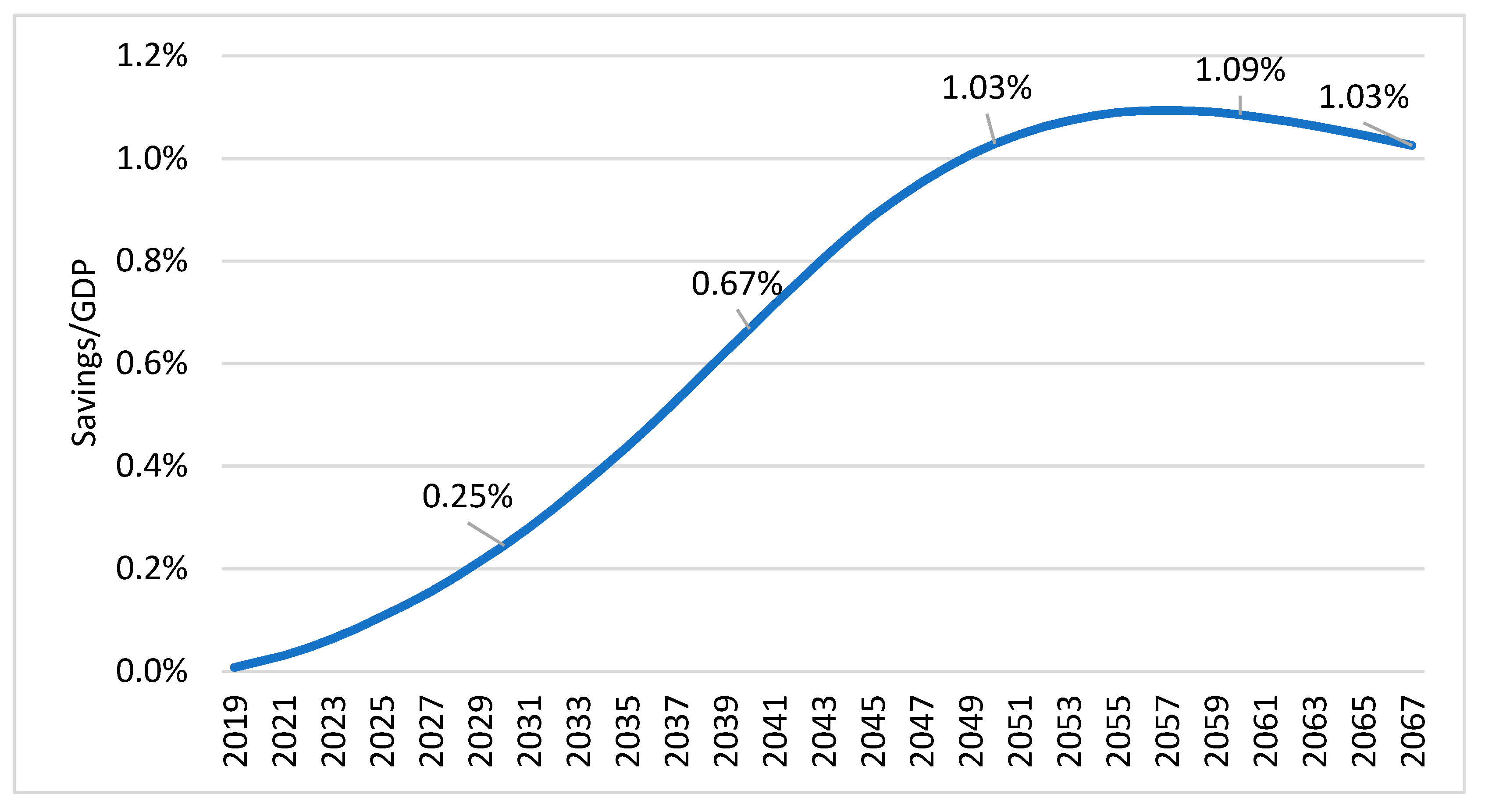
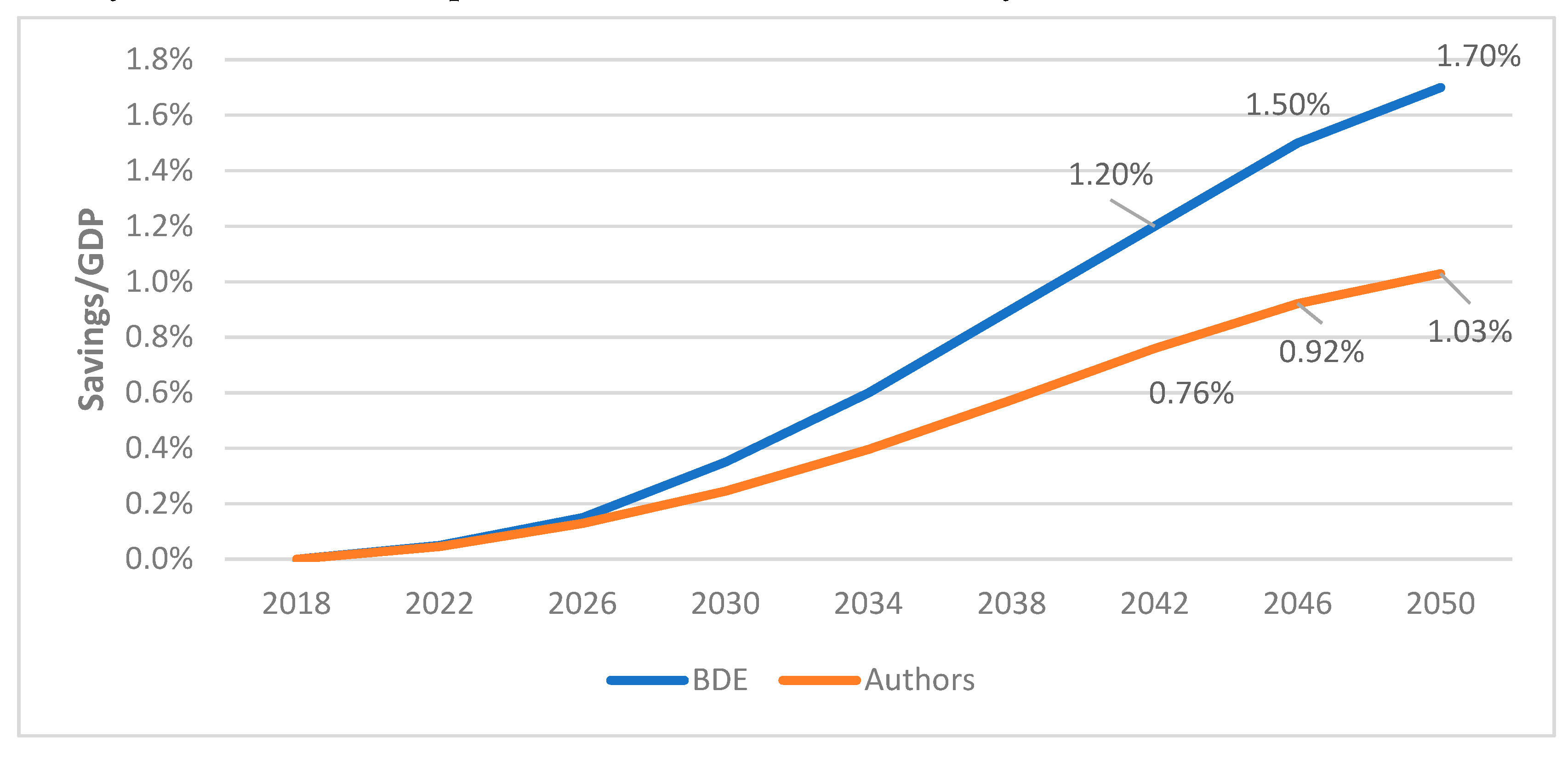
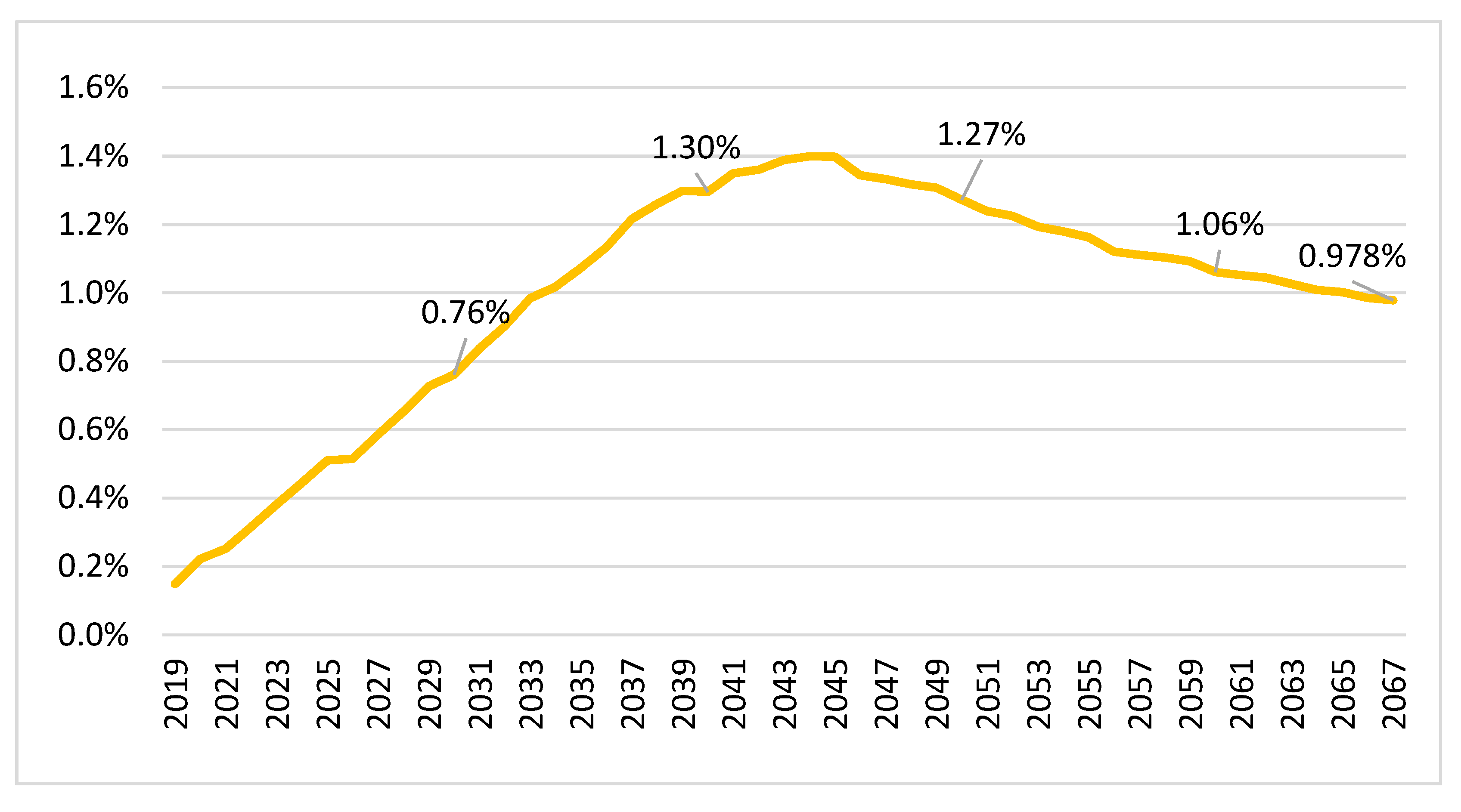
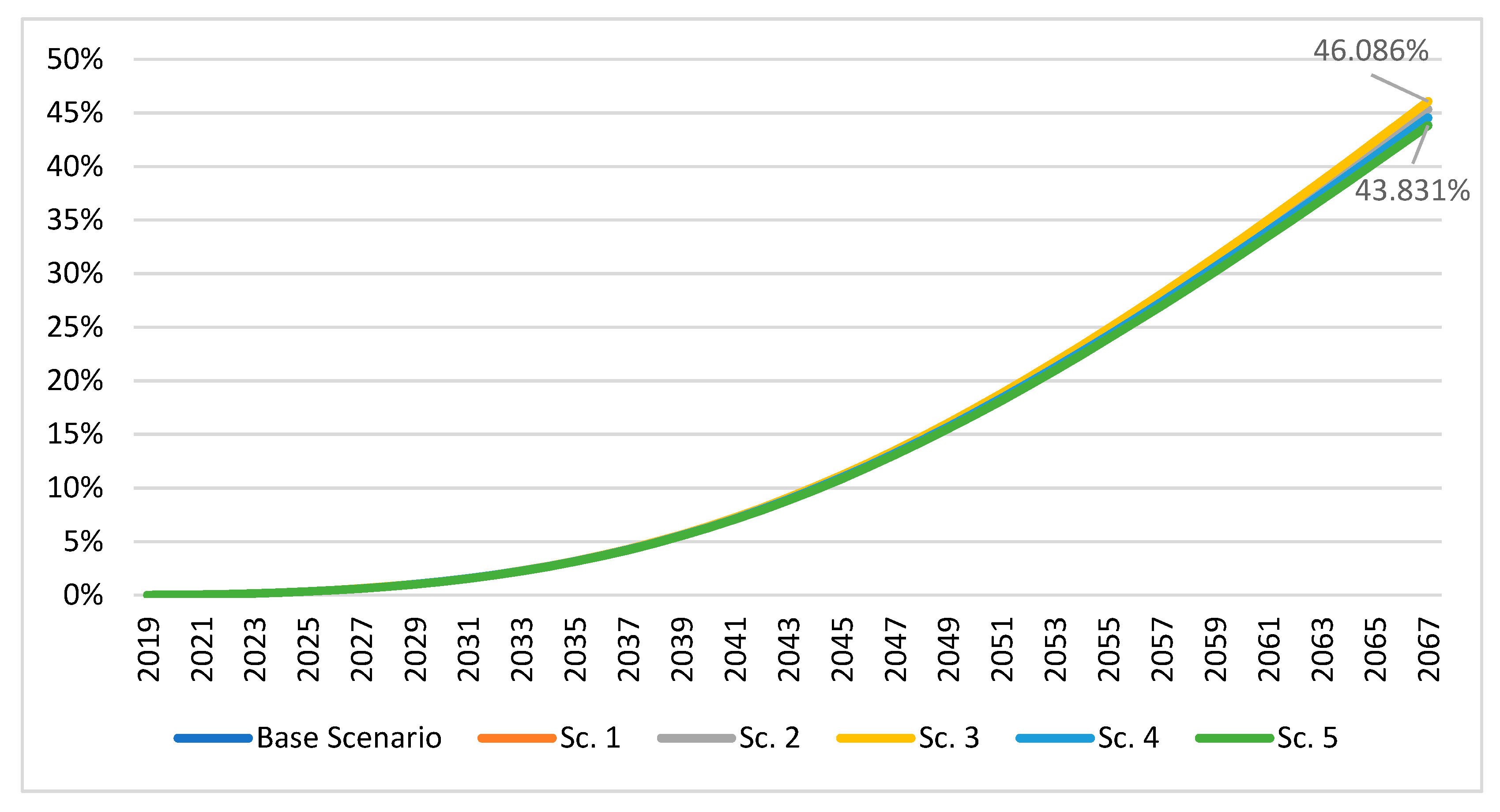
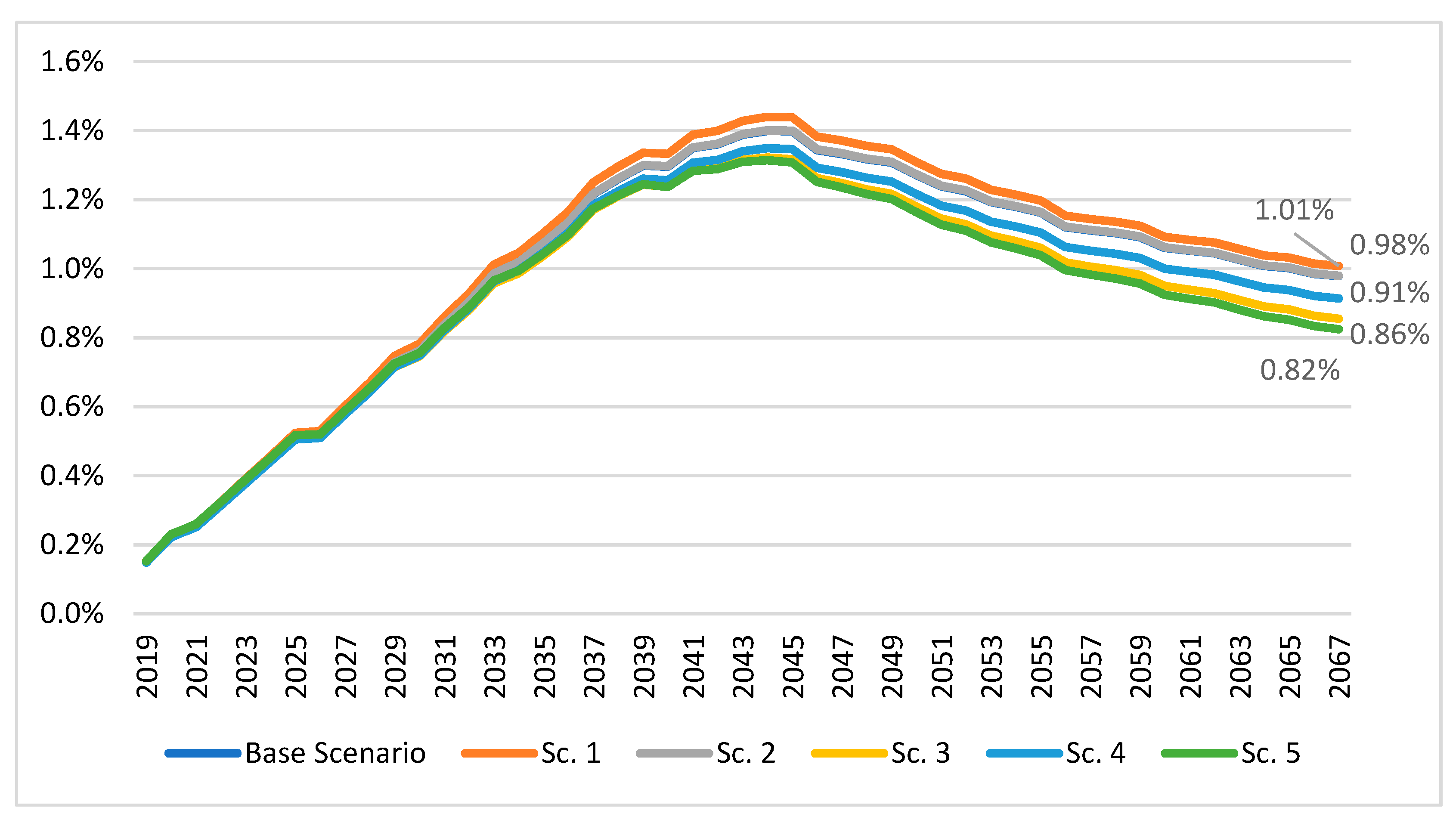
6.1. Estimation of Savings in Annual Retirement Pension Expenditure in Cash Terms

With the methodology outlined above and the working hypotheses considered, we show in Figure 5 the results, for the base scenario, of the annual savings in the retirement pension payroll that would be reaped from the application of the SF starting in 2019 in terms of GDP for the year of its calculation.

There is a clear growth during the first years of the analyzed period, reaching a maximum in 2057 at 1.094%, followed by a slight decline. In any case, the figure obtained in 2050 indicates a savings of 1.029% of the GDP for that year, almost the same as the 1.026% achieved in 2067.

The profile shown in Figure 5, with a growth that softens from 2035 and begins to decline from 2057, is due, above all, to the evolution of the number of new pensions, which in turn depends on two elements: first, the evolution of mortality (since a dynamic mortality table is used) and second, the evolution of the number of pensions, data that has been provided by Social Security.

The Banco de España (BDE) through Hernández de Cos et al. (2017) has also published the savings data generated by the application of the SF; however, these results would be overestimating the real impact of the SF because, as stated in the document, “For simplicity, it is assumed that the SF affects all pensions, not only retirement pensions”.

Figure 6 shows the difference between the BDE estimate and the one we calculated in this work. The data in the BDE document only went until 2040 but could be extended to 2050 with another document, Hernandez de Cos (2020). The BDE always shows greater savings on GDP, reaching a maximum of 65% higher, although it should be remembered that our calculations are made exclusively for the retirement pension and not for all as done by the BDE.

The Independent Authority for Fiscal Responsibility (AIReF (2019)), using the INE tables, in its assessment of the SF’s effect on pension expenditure, states that “The implementation of the Sustainability Factor implies containing an additional expenditure of 0.6% through 2048”, a value that in our case would be 0.982%, or 64% more than the AIReF projection, in part because the Authority uses older mortality tables.

We also thought it appropriate to show the cumulative effect on retirement pension savings that applying the SF would have, to give us a clearer idea of the importance of this automatic resetting mechanism. To this end, we chose to represent the value of the accumulated savings in 2019 fixed terms, relative to GDP of the same year, not including the payment of interest that could involve the indebtedness of the Social Security system nor updating the interest rate. Figure 7 shows that until 2050 the implementation of the SF would achieve a cumulative savings of 17.39% of GDP in 2019, reaching 33.24% in 2060 and more than 46% in 2067, which is the last year of the study.

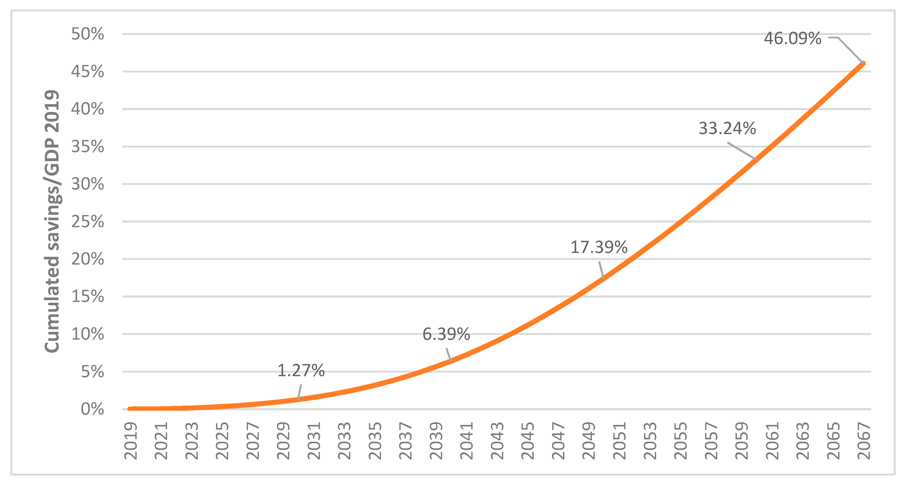
6.2. Estimation of Savings in Expenditures on Retirement Pensions in Terms of Accrual

Figure 8 shows the savings in present actuarial value with respect to the GDP of each year that is generated by the cohort that retires in that year if the SF is applied, compared to not applying the SF. For example, in 2050, the savings would be 1.27% of the GDP of that year, which could be understood as the extra amount that would have to be delivered in 2050 to be able to pay, for life, those retiring that year if the SF is not applied. This value is not comparable to that of the previous section because before we measured that effect in terms of cash and not accrual. The maximum would be reached in 2044 at 1.40% of the GDP of that year.

The profile shown in Figure 8 is similar to that of Figure 5, although the variations from one year to another are more similar in this case than in that of annual savings. This is because when the present actuarial value is calculated there is no “carry-over” of the previous values. This also means that Figure 8 is a less smooth function.

If we calculate the financial sum (updating according to expected inflation) of the present actuarial value of the savings for each year from 2019 to 2067 and divide it by the GDP of 2019, the result is 56.34%. That is, more than EUR 700,000 million (in 2019 euros) would have to be deposited today to secure the greater expenditure caused by not applying the SF to the cohorts of 2019–2067.

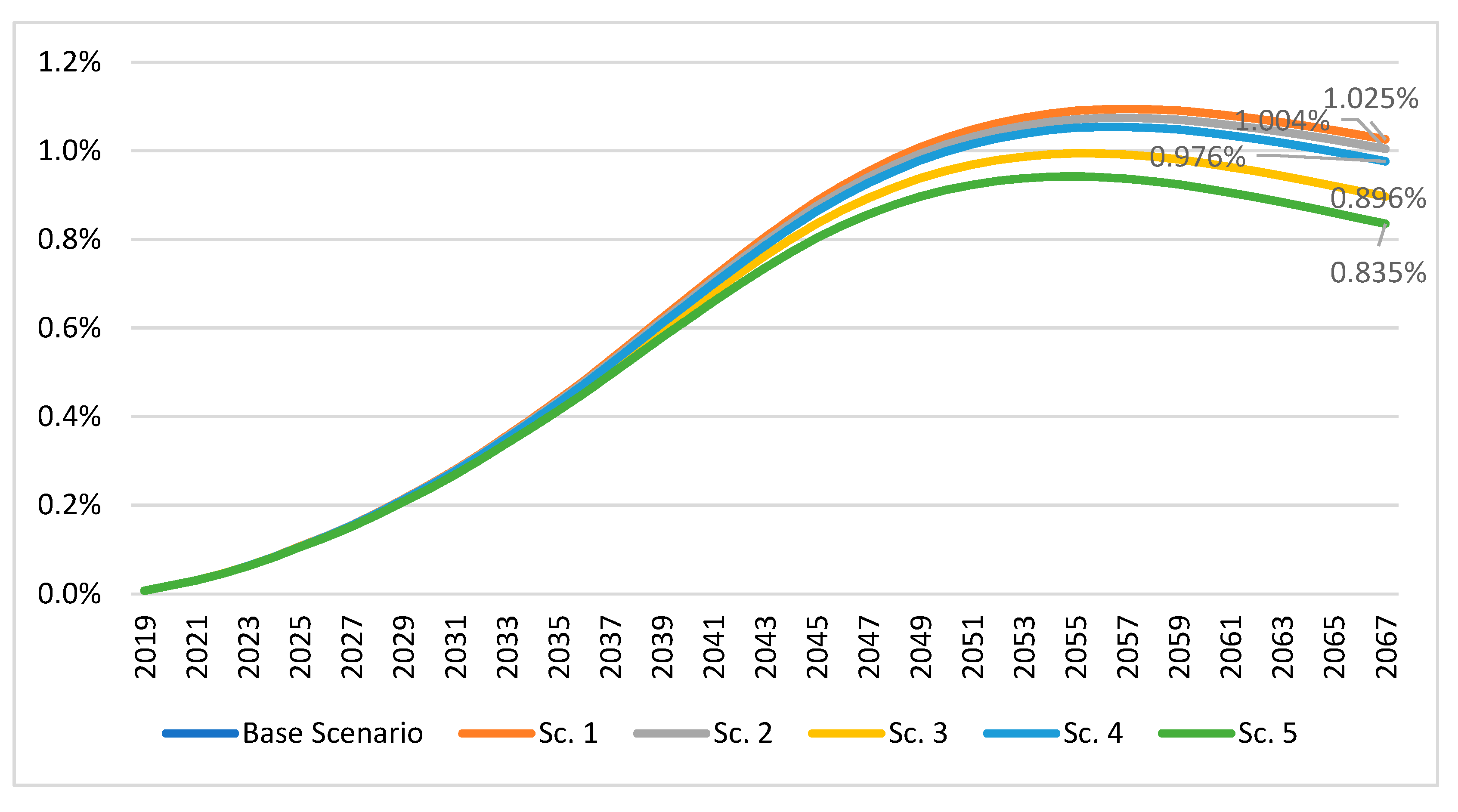
7. Sensitivity Analysis of the Working Hypotheses and the Effect of Delaying the Application of the Sustainability Factor

In this section, we will perform a sensitivity analysis with respect to the baseline scenario. The consequences of delaying the application of the SF are also analysed.

7.1. Modification of the Baseline Scenario

A series of variables that we have considered relevant will be taken into account. The values used in the different scenarios are showed in

Table 5. Hypotheses adopted for the sensitivity analysis.

Parameter	Baseline Scenario	Scenario 1	Scenario 2	Scenario 3	Scenario 4	Scenario 5
Interest rate	2%	1.8%	2%	2%	2%	1.8%
Inflation	1.6%	1.6%	1.6%	1.6%	1.6%	1.6%
α = Pension revaluation	1.6%	1.6%	1.44%	1.6%	1.6%	1.44%
GDP growth since 2021	Ageing Report	Ageing Report	Ageing Report	110% Ageing Report	Ageing Report	110% Ageing Report
β = Variation in the average pension benefit of new retirement registrations	1.411%	1.411%	1.411%	1.411%	1.27%	1.27%
Mortality tables	Eurostat	Eurostat	Eurostat	Eurostat	Eurostat	Eurostat

Source: Own elaboration.

. In all of them, the base scenario data were varied by 10% up and down. Scenarios 1 to 4 examine the variation of a single variable to determine its impact alone. Scenario 5 shows the joint impact of the four modified variables.

Figure 9 shows the impact of the SF on annual savings with respect to the GDP of each year. The baseline scenario overlaps with scenario 1 since the interest rate does not alter the valuation in cash terms. Regarding the rest of the variables, the one that least influences is the pensions revaluation (scenario 2), since in 2067 savings would go from 1.025% to 1.004%, while the variable that most modifies the results from the baseline scenario is the variation in GDP (scenario 3), which reduces annual savings to 0.896% of GDP. When we consider all the variables together (scenario 5), the savings would fall to 0.835% in 2067. The variations are not very large because we measure only the impact of the SF by modifying the different variables in the two expenditure projections considering the SF and not considering it.

In Figure 10, we show the accumulated savings from 2019 to the reference year, measured with respect to the GDP of 2019. The base scenario, the scenario 1 and the scenario 3 overlap, since the variation in neither the interest rate nor the GDP affects these last two scenarios, because the accumulated savings are being calculated against the GDP of 2019. The differences brought by the rest of the variables are small; the greatest difference is when the compared variable is the variation of the average benefit of new pensions, whose value in 2067 would go from 46.086% to 44.550%. In scenario 5, which jointly considers the two variables that modify the values of savings (pension revaluation and average benefit of new pensions), there is a somewhat stronger decrease, reaching 43.831% by the end. Therefore, the variation (taking into account that it is in the last year of analysis) is very small.

If we make the comparison taking into account the present actuarial value (Figure 11), the base scenario fully matches with scenario 2, which includes the variation in pension revaluation. There is an increase in savings when the interest rate decreases (scenario 1) because this updates future flows; this value would go from 0.978% to 1.01% in 2067. The variable that generates the greatest decrease in savings is the highest GDP growth (scenario 3), in which case the savings decrease by 0.86% in 2067. The variation of the average benefit of new pensions (scenario 4) is intermediate, at 0.91%. When considering all the variables together, savings would fall to 0.82%, though as we have mentioned, the decrease in the interest rate increases savings and therefore partially compensates for the effects of the other variables.

7.2. Delay in Applying the Sustainability Factor

Initially, it was planned that the SF would be implemented in 2019, but this did not happen, although it is possible that it will be applied in 2023. We also wanted to evaluate the impact of this delay on pension expenditures. We recalculated the SF assuming it would be applied in 2023, leaving the rest of the variables of the base scenario constant. This told us what effect the delay itself would have.

In 2050, savings in annual expenditures on retirement pensions in cash terms would drop from 1.03% to 0.72% of GDP that year17, while if the comparison is made in 2067, savings would drop from 1.03% to 0.83%. In view of these data, it should be noted that a delay of only 4 years in applying the SF will significantly lower the savings in pension spending: 0.31% of the GDP in 2050 and 0.20% in 2067.

8. Conclusions

One of the contributions of the work was the development of a complex model of expenditure projection for the Spanish retirement pension system, which has been designed specifically to adjust it to the available data. It has been structured by combining different instruments:

(a)

Microdata were used, obtained from the MCVL2018, with which we generated information on both new registrations of retirement pensions (new pensions) and on the total retirement pensions, by age and by gender.

(b)

Real aggregate data from the pension system on the total number of retirement pensions and their average benefit amount were used, which allowed complete extraction of the data without loss of information.

(c)

An actuarial method was used, with financial factors, survival probabilities, and annuities, which are essential to adequately project the evolution of the different cohorts of retirees, as well as to correctly value them quantitative terms.

(d)

A projection using financial methods was applied, complementing all the information with that obtained from the previous instruments.

We believe that the combination of four sub-models to achieve a model that performs a more precise adjustment of the desired objective is the first time that has been applied not only for Spanish data but also for data from other neighboring countries. Moreover, we consider that this method is well suited to the objective of the work, since it allows us to incorporate all the peculiarities of the pension system.

Another advantage is that the effect of SF has been isolated from the rest of the variables involved in pension expenditures. This has allowed us to conclude that applying the SF has significant effects on pension expenditure, since in 2050, this expenditure would decrease by 1.03% of the GDP of that year, with a slight growth until 2057, reaching 1.09%, after which it falls until 2067 to 1.03% of the GDP that year. Undoubtedly, this would relieve some of the stress on the sustainability of a pension system that currently presents significant problems.

The savings is more striking when we accumulate the effect since 2019. In this case, in 2050 an updated savings value of 17.39% of the 2019 GDP is reached, while in 2067, the cumulative real value of savings would reach 46.09% of the 2019 GDP.

We also thought it necessary to calculate the savings in terms of present actuarial value. That is, we calculated for each year what would be the single disbursement that would be necessary to meet the greater expense generated by each cohort of new retirees if the SF were not applied. The values obtained are 1.27% in 2050 and 0.98% in 2067. These data give us complementary information to the cash flow since they take into account the accrual of flows.

The sensitivity analysis carried out by modifying the base scenario shows that the variations proposed in the hypotheses do not significantly affect the results obtained. Thus, for example, in the case that four of the variables used in the projection were simultaneously modified, savings in 2050 would only decrease from 1.03% to 0.91% of GDP.

The same does not happen when we analyse the effect of a four-year delay in applying the SF, from 2019 to 2023: This would result in a significantly smaller expenditure reduction: just over 0.3% of the GDP in 2050.

The evolution of the data that we showed allows us to better understand the impact that the arrival of the Baby Boom generation will have at retirement age if the SF is applied or not. The impact is significantly greater, 64% more than projected by AIReF; therefore, we believe that the methods used for those projections should be reviewed. The BDE data are not comparable because their study applied the SF to all benefits.

All of the above allows us to conclude that not only should the SF designed for the Spanish pension system not be reversed but also that it should be implemented as soon as possible due to the large impact in delaying it until 2023.

Specifically, the application of the SF would achieve two objectives:

(a)

One, a significant savings in spending, which would either increase the sustainability of the system or allow the savings to be allocated to improve the situation of those receiving the fewest benefits.

(b)

Two, an increase in the intergenerational equity of the pension system by assigning individuals with the same work careers the same total sum in pensions, regardless of their year of retirement.

Obviously, a model that involves a high number of variables is always subject to changes in the projections, especially when they are made in the long term. We are aware of the limitations not only of this model but of any other one that can be implemented. But, on the other hand, the sensitivity analysis carried out in our work indicates that changes in the values of the different variables do not generate significant variations in the estimated savings.

It is very likely that the SF regulations in Spain will be reviewed in the coming months. In this case, our future research will focus on analyzing the effect that these measures may have on savings in pension expenditures.

References

1. AIReF. 2019. Spanish Independent Authority for Fiscal Responsibility. Opinión Sobre la Sostenibilidad del Sistema de Seguridad Social. Opinión 1/19. Available online: https://www.airef.es/wp-content/uploads/2019/OPINIONES/190109_Opinion_Seguridad-Social.pdf (accessed on 29 November 2020).
2. Alda, Mercedes, Isabel Marco, and Adrián Marzo. 2018. La reforma del sistema público de pensiones español: El factor de sostenibilidad. Revista de Finanzas y Política Económica 10: 25–43. [Google Scholar] [CrossRef] [Green Version]
3. Antn, Sorin Gabriel, Elena Toader, and Bogdan Firtescu. 2016. Does Risk Management with Derivatives Improve the Financial Performance of Pension Funds? Empirical Evidence from Romania. Transformations in Business & Economics 15: 565–79. [Google Scholar]
4. Barea, José, Maximino Carpio, and Eugenio Domingo. 1996. Escenarios de Evolución del Gasto Público en Pensiones y Desempleo en el Horizonte 2020. Bilbao: Fundación BBV Documenta. [Google Scholar]
5. Carone, Giuseppe, Per Eckefeldt, Luigi Giamboni, Veli Laine, and Stephanie Pamies. 2016. Pension Reforms in the EU since the Early 2000’s: Achievements and Challenges Ahead. European Economy Discussion Paper, 42. Available online: http://ec.europa.eu/economy_finance/publications/eedp/pdf/dp042_en.pdf (accessed on 29 November 2020).
6. Committee of Experts. 2013. Informe del Comite de Expertos Sobre el Factor de Sostenibilidad del Sistema Público de Pensiones. Available online: http://www1.seg-social.es/ActivaInternet/groups/public/documents/rev_anexo/rev_032187.pdf (accessed on 29 November 2020).
7. Da-Rocha, José-Marıa, and Francisco Xavier Lores. 2005. ¿Es Urgente Reformar la Seguridad Social. RGEA Research Group in Economic Analisis, Working Paper Series; Vigo: Vigo University. [Google Scholar]
8. Devesa-Carpio, José-Enrique, and Mar Devesa-Carpio. 2010. The cost and actuarial imbalance of pay-as-you-go systems: The case of Spain. Journal of Economic Policy Reform 13: 259–76. [Google Scholar] [CrossRef]
9. Devesa, José Enrique, Mar Devesa, Robert Meneu, Juan José Alonso, Inmaculada Domínguez, Borja Encinas, Francisco Escribano, Pablo Moya, Isabel Pardo, and Raúl del Pozo. 2016. La Revolución de la Longevidad y su Influencia en las Necesidades de Financiación de los Mayores. Madrid: Fundación Edad & Vida, Available online: https://www.vidacaixa.es/documents/51066/91055/estudio.pdf/4247f979-a9ac-05a9-ac42-3d319ea8ada7 (accessed on 29 November 2020).
10. Díaz-Giménez, Javier. 2014. Las Pensiones Europeas y sus Reformas Recientes. Documento de Trabajo nº 7. In Instituto BBVA de Pensiones. Madrid. Available online: https://www.jubilaciondefuturo.es/recursos/doc/pensiones/20131003/posts/2015-7-las-pensiones-europeas-y-sus-reformas-recientes-esp.pdf (accessed on 29 November 2020).
11. Díaz-Giménez, Javier, and Julián Díaz-Saavedra. 2017. The future of spanish pensions. Journal of Pension Economics & Finance 16: 233–65. [Google Scholar]
12. Duran, Almudena. 2007. La Muestra Continua de Vidas Laborales de la Seguridad Social. Revista del Ministerio de Trabajo y Asuntos Sociales 1: 231–240. [Google Scholar]
13. Economic Policy Committee, and Social Protection Committee from the European Commission. 2020. Joint Paper on Pensions 2019. Available online: https://europa.eu/epc/system/files/2020-01/Joint-Paper-on-Pensions-2019.pdf (accessed on 29 November 2020).
14. Encinas-Goenechea, Borja, Robert Meneu-Gaya, and María de la Cruz del Río. 2020. The Public Pension Systems and the Economic Crisis. In Economic Challenges of Pension Systems. A Sustainability and International Management Perspective. Edited by Marta Peris-Ortiz, José Alvarez-Garcia, Inmaculada Dominguez-Fabian and Pierre Devolder. Cham: Springer, pp. 57–80. [Google Scholar] [CrossRef]
15. European Commission. 2012. Libro Blanco, Agenda Para una Pensiones Adecuadas, Seguras y Sostenibles. Bruselas, COM (2012) 55 Final, February 16. Available online: http://eurlex.europa.eu/LexUriServ/LexUriServ.do?uri=COM:2012:0055:FIN:ES:PDF (accessed on 29 November 2020).
16. European Commission. 2018. The 2018 Ageing Report. Economic and Budgetary Projections for the 28 EU Member States (2016–2070). European Economy, Institutional Paper 079. Available online: https://ec.europa.eu/info/sites/info/files/economy-finance/ip079_en.pdf (accessed on 29 November 2020).
17. Eurostat Database. 2020. Available online: https://ec.europa.eu/eurostat/data/database (accessed on 29 November 2020).
18. Herce, José Antonio A., and Víctor Perez-Diaz, eds. 1995. La Reforma del Sistema Público de Pensiones en España. Servicio de Estudios de La Caixa, Colección Estudios e Informes, nº 4. Available online: https://www.caixabankresearch.com/sites/default/files/content/file/2016/09/ee04_esp.pdf (accessed on 29 November 2020).
19. Hernandez de Cos, Pablo. 2020. Retos del Envejecimiento de la Población. Desayuno de Trabajo con la Junta de Gobierno del Instituto de Actuarios Españoles. Madrid. Available online: https://www.bde.es/f/webbde/GAP/Secciones/SalaPrensa/IntervencionesPublicas/Gobernador/Arc/Fic/hdc270120.pdf (accessed on 29 November 2020).
20. Hernández de Cos, Pablo, Juan F. Jimeno Serrano, and Roberto Ramos. 2017. El sistema público de pensiones en España: Situación actual, retos y alternativas de reforma. In Documentos Ocasionales. Banco de España. Nº 1701. Available online: https://www.bde.es/f/webbde/SES/Secciones/Publicaciones/PublicacionesSeriadas/DocumentosOcasionales/17/Fich/do1701.pdf (accessed on 29 November 2020).
21. Hoyo, Lao. 2014. El factor de sostenibilidad el sistema público de pensiones y su entrada en vigor. El factor de equidad intergeneracional ajustado a la edad de acceso a la jubilación. Economía Española y Protección Social, 75–117. Available online: file:///C:/Users/USUARIO/Downloads/EEYPS%20VI%20-%202014%20-%203.pdf (accessed on 29 November 2020).
22. Lapuerta, Irene. 2010. Claves para el trabajo con la Muestra Continua de Vidas Laborales. In DemoSoc Working Paper. nº 2010-37. Barcelona: Universidad Pompeu Fabra. [Google Scholar]
23. Law 27. 2011. de 1 de Agosto, Sobre Actualización, Adecuación y Modernización del Sistema de Seguridad Socia. Published in BOE Num. 184 of August, 2. Available online: https://www.boe.es/eli/es/l/2011/08/01/27 (accessed on 29 November 2020).
24. Law 23. 2013. de 23 de Diciembre, Reguladora del Factor de Sostenibilidad y del Índice de Revalorización del Sistema de Pensiones de la Seguridad Social. Published in BOE Num. 309 of December, 26. Available online: https://www.boe.es/eli/es/l/2013/12/23/23 (accessed on 29 November 2020).
25. Spanish Continuous Sample of Working Lives. 2018. Available online: http://www.seg-social.es/wps/portal/wss/internet/EstadisticasPresupuestosEstudios/Estadisticas/EST211 (accessed on 29 November 2020).
26. Gaya, Robert Meneu, José Enrique Devesa Carpio, Mar Devesa Carpio, Amparo Nagore García, Inmaculada Domínguez Fabián, and Borja Encinas Goenechea. 2013. El factor de sostenibilidad: Diseños alternativos y valoración financiero-actuarial de sus efectos sobre los parámetros del sistema. Economía Española y Protección Social 63–96. Available online: file:///C:/Users/USUARIO/Downloads/EEYPS%20V%20-%202013%20-%203.pdf (accessed on 29 November 2020).
27. Pérez Alonso, María Antonia. 2016. El Factor de Sostenibilidad en España. Lex Social 6: 145–74. [Google Scholar]
28. Real Decreto-Law 5. 2013. de 15 de marzo, de Medidas Para Favorecer la Continuidad de la vida Laboral de los Trabajadores de Mayor edad y Promover el Envejecimiento Activo. Published in BOE Num. de 16/03/2013. Available online: https://www.boe.es/eli/es/rdl/2013/03/15/5/con (accessed on 29 November 2020).
29. Sanchez Martin, Alfonso. 2014. The automatic adjustment of pension expenditures in Spain: An evaluation of the 2013 pension reform. In Banco de España. Documento de Trabajo nº 1420. Available online: https://www.bde.es/f/webbde/SES/Secciones/Publicaciones/PublicacionesSeriadas/DocumentosTrabajo/14/Fich/dt1420e.pdf (accessed on 29 November 2020).
30. Serrano, Felipe, Miguel A. García, and Carlos Bravo. 2004. El Sistema Español de Pensiones. Un Proyecto viable Desde un Enfoque Economico. Barcelona: Ariel. [Google Scholar]
31. Social Protection Comitee from the European Commision. 2016. Review of Recent Social Policy Reforms: 2015 Report of the Social Protection Committee. Available online: https://op.europa.eu/en/publication-detail/-/publication/3aff6199-ca44-11e5-a4b5-01aa75ed71a1/language-en (accessed on 29 November 2020).
1
According to the most recent Eurostat data (Eurostat Database 2020), from years 2002 to 2018, the life expectancy at 65 years of age in the EU increased by 2.2 years and in Spain, one of the longest-living countries, by 2.5 years. This means that with each passing year, life expectancy grew by 1.65 and 1.88 months, respectively. In addition, according to the European Commission (2018), this increase in longevity will continue in the coming decades from 18 years for the EU as a whole in 2016 to 23.4 years in 2070.
2
Another type of reforms of the three-pillar system would be reforms focused on an additional private pillar and the different structure of the pension funds in Central and Eastern Europe (Anton et al. 2016).
3
4
For more details on the characteristics of these automatic resetting mechanisms, see Gaya et al. (2013), Carone et al. (2016), European Commission (2018), and Economic Policy Committee and Social Protection Committee from the European Commission (2020).
5
In fact, this automatic mechanism was introduced in the reform approved in 2011 (Law 27 2011), but it did not specify which parameter of the system would be affected by changes in life expectancy.
6
Later, we will present the valuation data of Hernández de Cos et al. (2017) and AIReF (2019), although both have some drawbacks.
7
The Continuous Work Lives Sample (MCVL) is a random, non-stratified sample with information from more than 1.2 million individuals, representing 4% of all those who were associated with Social Security during a given year. This database is published annually by Social Security. For more information on MCVL, please refer to: Duran (2007), Lapuerta (2010) and Pérez Alonso (2016).
8
See Gaya et al. (2013) for more on this topic.
9
Although the current legislation includes the name sustainability factor, in the work (Committee of Experts 2013) that gave rise to regulatory development, the name used was intergenerational equity factor.
10
11
It was not updated actuarially because we have been able to generate the data on new retirement rates, that is, how many individuals are retiring in 2020.
12
The rest of the benefits are not taken into account because, according to regulations in effect, the SF only applies to retirement pensions.
13
Calculations until 2067 are done because this spans a broad period of time that includes the end of the impact of the Baby Boom generation.
14
Actually, pension withdrawals can occur, according to Social Security data itself, for three reasons: “death”, “age or term”, and “other causes”. In the case of retirement, in March 2020, only 6.87% of total withdrawals were not death-related. This rate in July 2020 is 15.7%, which suggests that these variations are due to the effect of COVID-19.
15
Instead of the annualized five-year data set by the regulations.
16
For GDP growth in the base scenario, data from the Ageing Report (European Commission 2018) have been used.
17
On 28 September 2020, AIReF modified its demographic projections and updated its estimate of the sustainability factor, indicating that its 2023 application will mean an additional saving of 0.9 points of GDP in 2050, a figure somewhat higher than the result that we obtained.
Scheme 1. Evolution of annual retirement pension expenditures including the sustainability factor. Source: Prepared by the authors. Where Σ is the sum for each retirement age, distinguishing between men and women. No. Nt: number of new retirement pensions registered in year t. APt: average pension benefit of new retirement pensions registered in year t. SFt: sustainability factor applicable to new retirement pensions registered in year t. spxjt: probability that an individual of age xj will survive s periods beyond year t. α: annual pension revaluation. It is assumed to be constant in this scheme.
Risks 08 00134 sch001
Scheme 2. Evolution of the Present Actuarial Value (PAV) of the annual expenditure on retirement pensions with a Sustainability Factor. Source: Prepared by the authors. Σ: 2019 sum of all the values of the scheme. Nº Nt: number of retirement registrations produced in year t. APt: average pension benefit of new retirement pensions registered in year t. FSt: sustainability factor applicable to new retirement pensions registered in year t. vt: financial discount factor for t periods; that is, vt = (1 + i)−t. α: annual pension revaluation. It is assumed to be constant in this scheme. αatxj: present actuarial value of an annuity, variable in a geometric progression of ratio α, initially payable in year t, to an individual of age xj.
Risks 08 00134 sch002
Figure 1. Life expectancy at birth. INE and Eurostat tables. Source: Prepared by the authors.
Risks 08 00134 g001
Figure 2. Life expectancy at 67 years. INE, Eurostat, and Social Security retiree tables. Source: Prepared by the authors.
Risks 08 00134 g002
Figure 3. Sustainability factor 2018–2100, Eurostat tables. Source: Prepared by the authors.
Risks 08 00134 g003
Figure 4. Sustainability factor 2018–2067, Eurostat and Social Security tables.
Risks 08 00134 g004
Figure 5. Annual savings/GDP with the application of the SF. Source: Prepared by the authors.
Risks 08 00134 g005
Figure 6. Annual savings/GDP applying the SF. BDE and Authors. Source: Hernandez de Cos (2020) and prepared by author.
Risks 08 00134 g006
Figure 7. Cumulative savings, since 2019, over GDP for 2019, with the application of the sustainability factor. Source: Prepared by the authors.
Risks 08 00134 g007
Figure 8. Savings in PAV/GDP each year with the application of the SF. Source: Own elaboration.
Risks 08 00134 g008
Figure 9. Annual savings/GDP with the application of the SF. Various scenarios. Source: Own elaboration.
Risks 08 00134 g009
Figure 10. Cumulative savings since 2019/GDP 2019 by applying the SF. Various scenarios. Source: Own elaboration.
Risks 08 00134 g010
Figure 11. Savings in PAV/GDP each year, with the application of the SF. Various scenarios. Source: Own elaboration.
Risks 08 00134 g011