Tail Risk Transmission: A Study of the Iran Food Industry

Abstract

This paper extends the extreme downside correlation (EDC) and extreme downside hedge (EDH) methodology to model the interdependence in the sensitivity of assets to the downside risk of other financial assets under severe firm-level and market conditions. The model is applied to analyze both systematic and systemic exposures in the Iranian Food Industry. The empirical application investigates (1) which company is the safest for investors to diversify their investment, and (2) which companies are the “transmitters” and “receivers” of downside risk. We study the return series of 11 companies and the Food Industry index publicly listed on the Tehran Stock Exchange. The data covers daily close prices from 2015–2020. The result shows that Mahram Manufacturing is the safest to hedge equity risk, and Glucosan and Behshahr Industries are the riskiest, while Gorji Biscuit is central to risk transmission, and Pegah Fars Diary is the main “receiver” of risk in turbulent times.

1. Introduction

Iran is one of the largest economies in the Middle East and North Africa (MENA) region with abundant natural resources. The country has almost one-tenth of the world’s oil, and one fifth of its natural gas reserves, with large mineral deposits which include copper, lead, zinc, Iron ore, and decorative stones. The agricultural sector of Iran is also vital to the country’s economy as it contributes to export earnings while ensuring food security, and serves as a major source of employment. Since the 1990s, the agricultural sector has continued to be the fastest-growing sector of the country (Stads et al. 2008). However, in an environment with increasing population and consumption, against a backdrop of shrinking land and water resources, there are concerns about the inability of the agricultural sector to provide food security to sustain the ever-increasing demand, which could lead to food crises and price hikes (Mesgaran et al. 2017). To mitigate these possible future occurrences, most developing countries, including Iran, must address the problem of agricultural financing through investment in food production (Nikabadi and Nouri 2017).

In recent years, to meet the desired food security, there has been an increase in the emergence of the Food and Conversion Industry for processing, preparing, preserving, and packaging of foodstuffs, in many developing countries, including Iran. Again, a key challenge facing these companies is access to capital to finance their operations. It is well known that in most emerging and developed economies, the stock market plays a significant role in economic growth. Therefore, by allowing these Food and Conversion Industries access to the stock market can improve the capital input allocation which would enhance productivity and contribution to the country’s economy (Amiri et al. 2009; Durnev et al. 2004).

Although the stock market will be convenient to raise capital for food manufacturing companies, there are many factors that directly/indirectly affect stock performance and causes uncertainty in stock price movements. One such factor is the “risk” of a stock, and potential investors are usually concerned with the trade-off between expected returns and risk associated with investment decisions (Bera and Kannan 1986; Puspitaningtyas 2018; Scott and O’Brien 2003). The first type of risk to consider is “systematic”—the sensitivity of the performance of an asset to a market crash. This type of risk is unavoidable in the sense that as long as a company operates in a given market, any shock that affects the market will definitely impact the performance of an individual asset. The second type of risk to consider is “systemic”—the inherent vulnerability of the system that propagates initial shocks leading to the failure of many institutions, whose cascading effects may endanger the whole system (see Battiston et al. 2012; Billio et al. 2012; Diebold and Yilmaz 2014). The financial crisis of 2008–2009 showed that shocks can spread from one market to institutions operating in different markets, causing widespread losses. This type of risk can be diversified. The third type of risk to consider in addition to systematic and systemic is “downside risk”. Stock markets often experience sudden and extreme events that trigger downside price movements, and investors are highly concerned about the performance of their assets in such circumstances. Many studies have documented the considerable impact of downside (tail) risk on expected returns (see Barro 2006; Gabaix 2012; Gillman et al. 2015; Rietz 1988; Wachter 2013).

In this paper, we study the sensitivity of assets to the downside risk of other financial assets under severe firm-level and market conditions. It is well known that in turbulent times some assets usually perform badly while others have mild reactions. Assets that react mildly are often desirable and usually, sell at a premium. We study these reactions via two recently proposed econometric techniques for tail risk measurement, i.e., the extreme downside hedge (EDH) and extreme downside correlation (EDC) (see Harris et al. 2019). The EDC is a non-parametric correlation-based measure, while EDH is a parametric measure of the sensitivity of a stock’s return to downside risk in the market and/or other competing stocks (Ahelegbey et al. 2020). We summarize the downside reactions among companies via a network model—the use graphs to represent statistical relationships (Lauritzen 1996). The network summarizes the complex channels of reactions by using nodes to represent companies and edges to describe the statistical relationships between pairs of companies. By ranking companies via network centrality measures, we identify the safest from the riskiest companies, as well as the “transmitters” and “receivers” of risk in a downturn.

The contributions of this paper is manifold. First, we contribute to the literature on financial risk by considering a model that combines tail risk with systemic and systematic risks. Secondly, we contribute to the expanding stream of literature on the relationship between tail risk and asset returns (Almeida et al. 2017; Chabi-Yo et al. 2018; Van Oordt and Zhou 2016). Van Oordt and Zhou (2016) studied a systematic tail risk measure that captures the sensitivity of asset returns to market returns conditional on market tail events. Almeida et al. (2017) analyzed a tail risk measure based on the risk-neutral excess expected shortfall of a cross-section of asset returns. Chabi-Yo et al. (2018) studied lower tail dependence (LTD) systematic tail risk based on estimating the sensitivity of an individual asset to a market crash. Our third contribution is an empirical exercise that aims at investigating the reaction of food companies to systemic and systematic risk in downturn situations. Our goal is to identify: (1) which companies are the safest for investors to diversify their investment; and (2) which companies are risk “transmitters” and “receivers” in turbulent times.

We apply our methodology to the return series of 11 companies and the Food Industry index listed on the Tehran Stock Exchange. Closely related to our study are Abbasi et al. (2012); Afrooz et al. (2010); Akbari et al. (2020); Azad et al. (2013); Hajiha et al. (2011); Hosseini et al. (2012); Hosseininia and Ramezani (2016); Naeini et al. (2019). Our application, however, differ from these studies in terms of model formulation. The result shows that Mahram Manufacturing is the safest stock to hedge equity risk, Glucosan and Behshahr Industries are the riskiest, while Gorji Biscuit is critical to risk transmission, and Pegah Fars Diary is the main “receiver” of risk in turbulent times.

The paper is organized as follows: Section 2 presents our proposed methodology. For our empirical application, we present a description of the data and report the results in Section 3 and Section 4 concludes the paper with a brief discussion and suggestions for future research.

2. Methodology

In this section, we briefly present the background to network models. Next, we describe our extension of the extreme downside correlation (EDC) and the extreme downside hedge (EDH) measures, aimed at modeling tail risk dependence among return series of assets.

2.1. Background: Network Models

A network model is a convenient class of multivariate analysis that uses graphs to represent statistical models (Lauritzen 1996). They are formally represented by $(G,\theta )\in (\mathcal{G}\times \Theta )$, where G is a graph of relationships between variables, $\theta$ is the model parameter, $\mathcal{G}$ is the space of graphs and $\Theta$ is the parameter space. The graph, G, is defined by a set of vertices (nodes/variables) joined by a set of edges (links), describing the statistical relationships between a pair of variables. A typical multivariate multiple regression model is given by

$$\begin{array}{c}\hfill Y=BX+U\end{array}$$

(1)

where $X=(X_1,\dots ,X_n)$ and $Y=(Y_1,\dots ,Y_n)$ are vector of exogenous and response variables respectively, B is a coefficient matrix and U is a vector of errors typically assumed to be multivariate normal. In this example, relationships between X and Y can be summarized by a weighted ($A^W$) or unweighted adjacency matrix ($A^U$), where $A_{ij}^W$ or $A_{ij}^U$ is such that

$$\begin{array}{c}\hfill \begin{array}{ccccc}{A}_{ij}^W=0\hfill & \Rightarrow \hfill & A_{ij}^U=0\hfill & \Rightarrow \hfill & X_j\cancel{\to }{Y}_i\hfill \\ A_{ij}^W=B_{ij}\in \mathbb{R}\hfill & \Rightarrow \hfill & A_{ij}^U=1\hfill & \Rightarrow \hfill & X_j\to Y_i\hfill \end{array}\end{array}$$

(2)

where $X_j\cancel{\to }{Y}_i$ means that $X_j$ does not influence $Y_i$.

A key feature of network models in contagion analysis is their usefulness in ranking systemically important institutions by identifying firms whose features are critical to the robustness/fragility of the system. We briefly present some standard network summary methods used in this study.

2.1.1. Degree Centrality

Degree centrality can be computed as unweighted/weighted in-degree and out-degree. Let $A=\{A^U,A^W\}$, then the in-degree of node-i, ${\overleftarrow{D}}_i$, and out-degree of node-j, ${\overrightarrow{D}}_j$, is given by

$$\begin{array}{ccc}\hfill {\overleftarrow{D}}_i=\sum _j{A}_{ij},& \hfill & \hfill {\overrightarrow{D}}_j=\sum _i{A}_{ij}\end{array}$$

(3)

where ${\overleftarrow{D}}_i$ counts the number of links directed towards node-i, while ${\overrightarrow{D}}_j$ is the number of links going out of node-j. If A is bi-directed (or undirected), then the in-degree of node-i is equal to its out-degree, which can be simply referred to as the degree of node-i.

2.1.2. Eigenvector Centrality

Eigenvector centrality can also be computed in terms of unweighted or weighted hub/authority centrality. Following the notation, $A=\{A^U,A^W\}$, the hub and authority centrality measures assign a score to nodes by solving the following:

$$\begin{array}{ccc}\hfill \left(A^{\prime }A\right)h={\lambda }_{h}h,& \hfill & \hfill \left(A{A}^{\prime }\right)a={\lambda }_{a}a,\end{array}$$

(4)

where h and a are the hub score and authority score eigenvectors, corresponding to ${\lambda }_h$ and ${\lambda }_a$, the largest eigenvalues of $A^{\prime }A$ and $A{A}^{\prime }$ respectively. If A is a bi-directed adjacency matrix, then $A^{\prime }=A$, which means that ${\lambda }_h={\lambda }_a$ and the hub score of the network is the same as the authority score, which is generally referred to as the eigenvalue centrality score.

From a financial contagion viewpoint, nodes with the highest in-degree are liable to be influenced and those with high out-degree are “influencers”. Nodes with high hub scores indicate high “transmitters” of risk, while high authority score nodes are “receivers” of risk. If the underlying network is undirected, then the “influencers” are also liable to be influenced, and the risk “transmitters” are also risk “receivers”.

2.1.3. Network Visualization

To visualize the network structure, we position the nodes in network via eigen-decomposition of $\Omega ={(I+A^W)}^{\prime }(I+A^W)$, whose $ij$-th entry can be parametrized as:

$$\begin{array}{cc}\hfill {\Omega }_{ij}& ={\left(U\mathsf{\Lambda }{U}^{\prime }\right)}_{ij}\hfill \end{array}$$

(5)

where ${\Omega }_{ij}$ is the i-th row and the j-th column of $\Omega$, $\mathsf{\Lambda }=\mathrm{diag}({\lambda }_1,\dots ,{\lambda }_r)$, is a diagonal matrix of eigenvalues, U is a $n\times r$ coordinate matrix of n points in an r-dimensional system such that $U_{i,:}$ denotes the i-th row of U (i.e., the coordinates of i-th node). These coordinates describe a spatial position of the firms in a financial network which can be very useful for their interpretation (see Ahelegbey et al. 2017; Ahelegbey and Giudici 2020; Hoff 2008).

2.1.4. Hierarchical Clustering—Node Segmentation

Hierarchical clustering is a technique for decomposing a network into community structures where nodes with similar attributes form a group, and nodes in two different groups have dissimilar characteristics. In this application, we compute the Euclidean distance between the latent coordinated of the nodes and apply the median weighting function, where the distance between two clusters is defined as the weighted distance between the centroids, with the weight being proportional to the number of individuals in each group. See Clauset et al. (2004); Fagiolo (2007) for further discussion.

2.2. Extreme Downside Correlation (EDC)

The EDC is a correlation-based technique that measures the marginal relationship between a pair of continuous variables, focusing on the tail of their joint return distributions. It is a non-parametric measure of tail risk co-movement of financial assets. Let $Y_{i,t}$ be the returns of assets i (or $Y_i$) at time t and denote with ${\mu }_i$ the historical mean of asset i. The $ED{C}_{\tau ,ij}$ measures the tail correlation between assets i and j given by

$$\begin{array}{c}ED{C}_{\tau ,ij}=\frac{Cov(Y_{\tau ,i},Y_{\tau ,j})}{\sqrt{Cov(Y_{\tau ,i},Y_{\tau ,i})}\sqrt{Cov(Y_{\tau ,j},Y_{\tau ,j})}}\end{array}$$

(6)

where $Cov(Y_{\tau ,i},Y_{\tau ,j})$ is the covariance between $Y_{\tau ,i}$ and $Y_{\tau ,j}$, $Y_{\tau ,i}$ is the left-side $\tau$-quantile of the standardized distribution on $Y_i$, $\tau \in (0,1)$, and $F_X\left(\tau \right)=Pr(Y_i\le \tau )$ is the cumulative distribution function (CDF) of $Y_i$. The value of $\tau$ defines the percentage confidence level, $100(1-\tau )\%$. If $j=m$ is a market index, then $ED{C}_{\tau ,im}$ captures the systematic relationship between asset-i and the market.

The tail of the return distribution technically corresponds to either extremely low gains (left tail) or very high returns (right tail). Following standard applications, we set our focus on the left tail to study the co-movement in returns of assets during stressful times which are usually characterized by losses. Following standard practice, we use the $\tau =5\%$ quantile level which corresponds to a 95% confidence level in our empirical application. We also conduct robustness checks with other $\tau$-quantile levels to validate the sensitivity of the findings.

2.3. Extreme Downside Hedge (EDH)

The extreme downside hedge (EDH) measures the sensitivity of returns to innovations in the tail risk of the market and/or of other counterparties. The variables of interest for the EDH model are the return series of the assets and a measure of innovation in the tail risk of the conditioning set of variables. Recent measures for assessing the riskiness of assets is the expected shortfall (also referred to as conditional value at risk—CoVaR or CVaR) (see Adrian and Brunnermeier 2016; Alexander 2009; Bali et al. 2009).

Let $Y_t=(Y_{1,t},\dots ,Y_{n,t})$ be n-variable vector of return observations at time t, where $Y_{i,t}$ is the time series of asset-i at time t. Let $Y_{\tau ,i}$ denote the left-side $\tau$-quantile of the distribution on $Y_i$, for $\tau \in (0,1)$. Following Rockafellar and Uryasev (2002) and Gaivoronski and Pflug (2005), we compute the $CVa{R}_{\tau }\left(Y_i\right)$ as a proxy for the tail risk by

$$\begin{array}{c}CVa{R}_{\tau }\left(Y_i\right)=\lambda E\left(Y_i|Y_i<Y_{\tau ,i}\right)+(1-\lambda )Y_{\tau ,i}\end{array}$$

(7)

where $\lambda =\frac{1}{\tau }{F}_X\left(\tau \right)$, $F_X\left(\tau \right)=Pr(Y_i\le Y_{\tau ,i})$ is the CDF of $Y_i$. $CVa{R}_{\tau }\left(Y_i\right)$ calculates the weighted average of the losses that occur beyond $Y_{\tau ,i}$, the value at risk point, in a distribution. We denote with $CVa{R}_{i,t}$—the $CVa{R}_{\tau }\left(Y_i\right)$ at time t. We employ $\Delta CVaR$ as a proxy for the innovation in the tail risk.

Following Harris et al. (2019), we start the EDH model with the systematic tail risk of an asset as the sensitivity of returns of asset-i with respect to $\Delta CVaR$ of the market index as

$$\begin{array}{cc}\hfill Y_{i,t}& ={\alpha }_i+{\beta }_{i|m}\Delta CVa{R}_{m,t}+{ϵ}_{i,t}\hfill \end{array}$$

(8)

where $\Delta CVa{R}_{m,t}=CVa{R}_{m,t}-CVa{R}_{m,t-1}$, ${\alpha }_i$ is the intercept, ${ϵ}_{i,t}$ is the error term, and ${\beta }_{i|m}$ is the response of the asset returns to changes in market tail risk. The vector of error term ${ϵ}_t=({ϵ}_{1,t},\dots ,{ϵ}_{n,t})$ is assumed to be multivariate normal.

The EDH for systematic risk in (8) expresses the “contagion” effect of the market tail risk on asset returns. It does not, however, capture other channels such as exposure to the tail risk of other assets. This application extends the EDH to consider a “systemic” version that estimate the sensitivity of the returns of a single index to the innovation in the CVaR of other indices. More formally, we can define the single index model of the EDH systemic risk by

$$\begin{array}{cc}\hfill Y_{i,t}& ={\alpha }_i+\sum _{i\ne j=1}^{n-1}{\beta }_{i|j}\Delta CVa{R}_{j,t}+{ϵ}_{i,t}\hfill \end{array}$$

(9)

where $\Delta CVa{R}_{j,t}=CVa{R}_{j,t}-CVa{R}_{j,t-1}$, ${\beta }_{i|j}$ is the response of the stock return of asset-i to changes in the tail risk of other assets.

A further approximation is a mixed EDH models that combines the right-hand side of (8) and (9) in the single index model. Thus, the mixed covariates model is a combined systemic and systematic representation given by

$$\begin{array}{cc}\hfill Y_{i,t}& ={\alpha }_i+\sum _{i\ne j=1}^{n-1}{\beta }_{i|j}\Delta CVa{R}_{j,t}+{\beta }_{i|m}\Delta CVa{R}_{m,t}+{ϵ}_{i,t}\hfill \end{array}$$

(10)

3. Empirical Findings

We apply our proposed methodology to the return series of 11 companies and the index for the food industry, all listed on the Tehran Stock Exchange. The data covers the period from 5 October 2015 to 19 April 2020. The choice of the Iranian Food Industry is motivated by the relevance of Iran in the Middle East and North Africa (MENA) region and its food industry widely recognized as a “sunrise industry”. This description is due to the huge potential in the enlistment of the agricultural economy, the creation of large-scale processed food manufacturing, the food chain facilities, and the generation of employment and export earnings. As a result, it can be considered to be one of the largest industries in Iran. The development of this industry would also increase the demand for agricultural products in food processing and reduce the level of waste (Afrooz et al. 2010). Despite the essential role of the industry, it has not received much attention as compared to that of the financial sector.

Table 1. Company Profile in terms of location and products.

No.	Name	Code	Location	Products
1	Behshahr Industrial Company	BEH	Tehran	All kinds of vegetable oil
2	Glucosan Company	GLN	Tehran	Process corn
3	Gorji Biscuit Company	GOJ	Tehran	Biscuit, Wafer, Cracker and Cookie
4	Kalber Dairy Company	KLR	Tehran	Diary products
5	Mahram Manufacturing Company	MHM	Tehran	Mayonnaise, sandwiches, honey, olives
6	Margarine Company	MRN	Tehran	Herbaceous oil, soybean oil, frying oil
7	Minoo Industrial Company	MIN	Tehran	Biscuit, Carbonated drinks and Cookies
8	Pars Minoo Industrial Company	PMI	Tehran	Chocolate, Cookie, Soft Drinks, Syrup
9	Pegah Fars Dairy Company	PFC	Shiraz	Milk and Dairy products
10	Salemin Factory	SLM	Tabriz	Biscuit, Chocolate and Confectionery products
11	West Azarbaijan Pegah Dairy	AZP	Urmia	Diary Products
12	Food Industry Index	FI	Tehran	Food Products

presents a profile of the companies in terms of location and products.

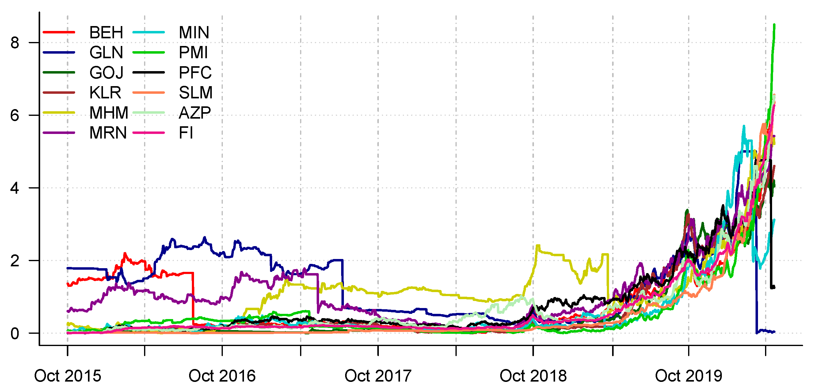
Figure 1 reports the time series of the daily index closing prices, on a logarithmic scale. Due to differences in values, we scale the prices to a zero mean and unit variance and add the absolute minimum value of each series to avoid negative outcomes. This standardizes the scale of measurement for the different series.

Let $P_{i,t}$ be the daily close price of company i on trading day t. We compute the return series as the 30-day percentage changes in the closing prices, i.e.,:

$$Y_{i,t}=100\left(\frac{P_{i,t}-P_{i,t-30}}{P_{i,t-30}}\right)$$

Table 2. Summary statistics of 30-day return series of the companies (October 2015 to April 2020).

Code	Mean	Sdev	Min	Max	Skew.	Ex.Kurt
BEH	2.8655	26.3890	−112.4748	82.0604	−1.7741	7.8269
GLN	−3.8449	48.1351	−285.9472	69.6142	−4.0990	20.4928
GOJ	6.4953	16.7188	−28.7854	89.2357	1.6114	3.7200
KLR	7.3899	21.9543	−39.6847	114.5958	1.4579	3.0709
MHM	5.2630	19.8725	−80.8469	63.3660	−0.3134	2.6338
MRN	4.4412	22.5201	−74.8406	85.4551	−0.1246	0.7690
MIN	4.4642	23.0606	−87.6150	62.0337	−0.4916	2.0921
PMI	7.5050	24.1774	−60.5344	102.8489	0.5807	2.0994
PFC	8.2288	20.7224	−101.7980	64.6445	0.0065	1.9441
SLM	11.4875	18.6729	−16.3660	82.4291	1.2085	0.7997
AZP	7.7350	21.4221	−56.4672	63.8704	0.1092	−0.0489
FI	7.8959	13.9899	−26.8253	59.3385	1.0293	0.5462

presents the summary statistics of the 30-day return series of the companies. It shows that on average the 30-day returns are quite different from zero and exhibit different variability in terms of standard deviations. In particular, Glucosan Company (GLN) is the riskiest with highest variability, followed by Behshahr Industrial Company (BEH). Gorji Biscuits Company (GOJ) reported the lowest variability among the companies. The skewness of the 30-day returns of the companies varies between −4.1 and 1.61, with most companies exhibiting moderate skewness. The reported excess kurtosis varies from −0.05 to 20.5. Except for West Azarbaijan Pegah Diary (AZP) recording a negative excess kurtosis. Majority of the companies displayed a platykurtic behavior (excess kurtosis $<3$).

A summary of Table 2 based on the mean-variance relationship of stock returns shows that the Salemin Factory (SLM) has the highest average monthly returns (11.4875) and relatively lower risk (18.6729 of returns) compared to the rest over the full sample period. The only stocks with a much lower risk than SLM are the Food Industry index (FI) and the Gorji Biscuits Company (GOJ); however, both indices have a relatively lower average monthly returns compared to SLM. Glucosan Company (GLN), on the other hand recorded the lowest average month returns (−3.8449) with the highest risk (48.1351). It is followed by Behshahr. Thus, in normal times, investing in Salemin Factory (SLM) will yield high returns and lower risk for investors.

In the rest of this section, we present the results of the Extreme Downside Correlation analysis in Section 3.1 and Extreme Downside Hedging in Section 3.2.

3.1. Extreme Downside Correlation Analysis of Iran’s Food Industry

We analyze the tail correlations by daily $VaR$ via a 30-period rolling estimation of daily returns. Preliminary estimation of the $VaR$ of some returns produced constant observations overtime. We used a Monte Carlo Sampling algorithm to draw 1000 samples of the loss vector given the mean and standard deviation of the loss distribution. This exercise is replicated 10 times to estimate the $VaR$ series and the EDC model. 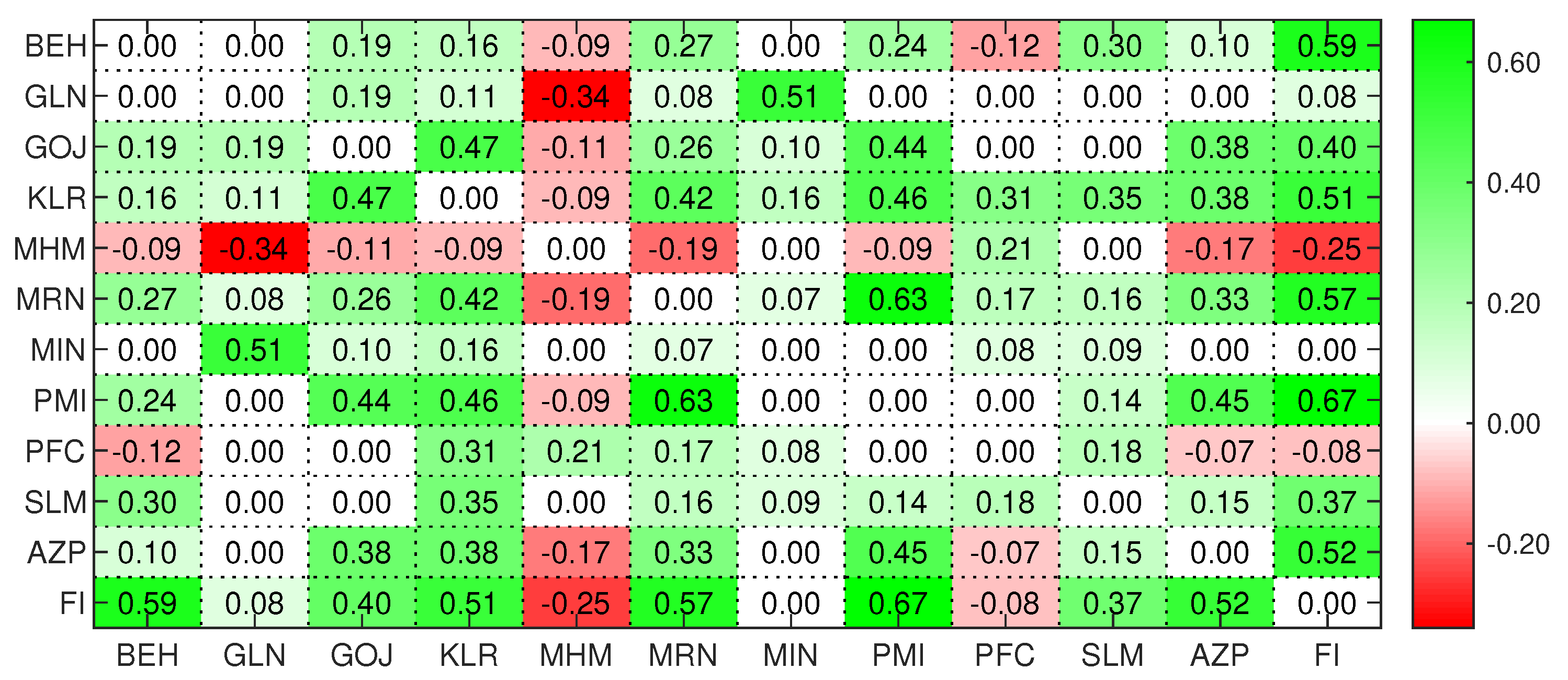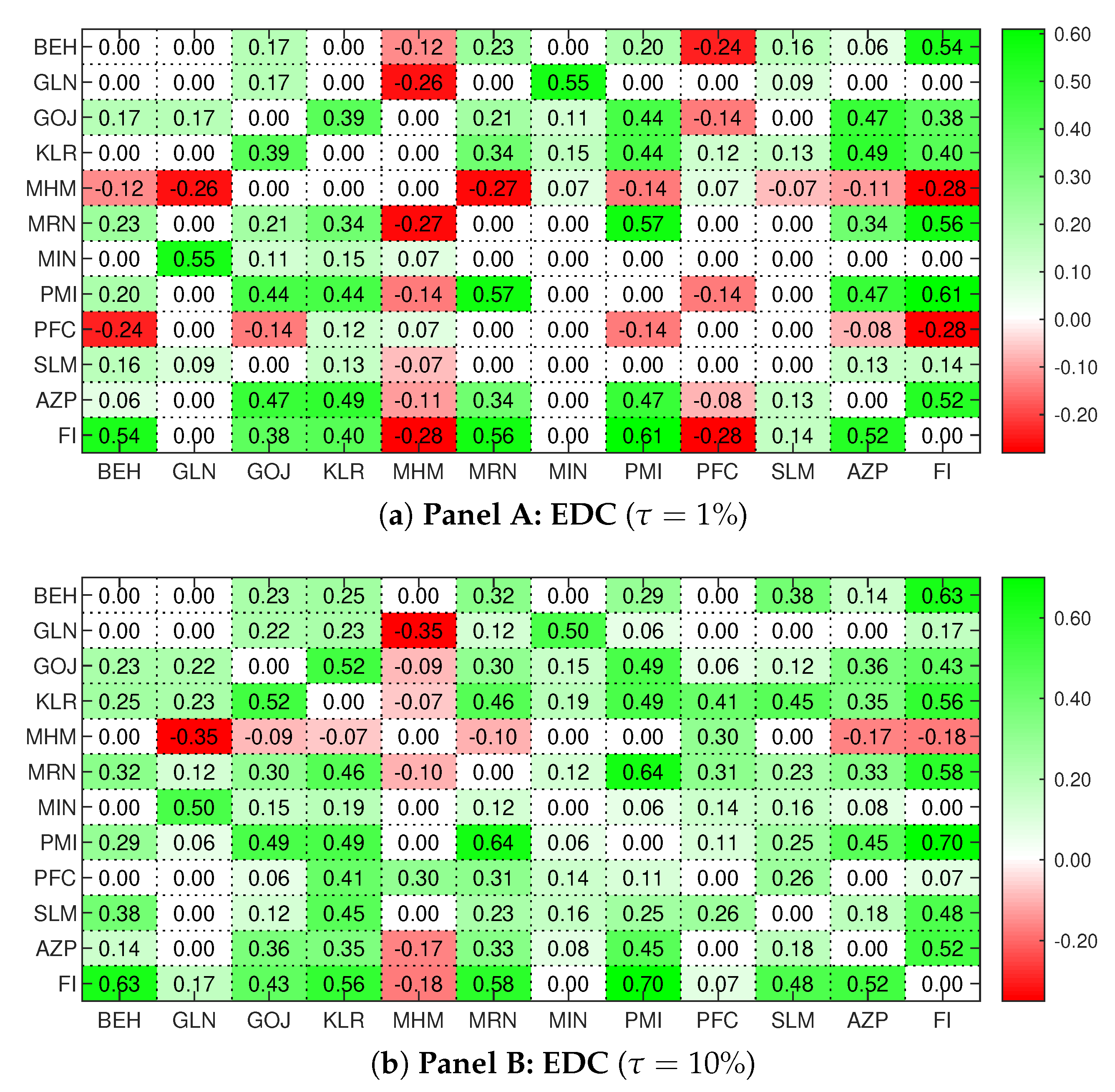Figure 2 report the result of the extreme downside correlation (EDC) matrix at $5\%$-quantile level. Correlations coefficients lower than the 5% significance level are set to zeros. A systematic analysis of the results focuses on the co-movement between the Food Industry index (FI) and the rest, while the systemic analysis concentrates only on the companies excluding the industry index.

3.1.1. Systematic EDC Analysis

From a systematic perspective, Figure 2 reveals that the downside risk of the market strongly correlates with PMI (a correlation coefficients around 0.67), followed by BEH, MRN, and AZP. Companies like MIN, PFC, and GLN are, however, strongly uncorrelated with the market, while MHM is the only negatively correlated company with the market.

Table 3. Ranking tail correlation coefficients between companies and Food Industry index. The light (dark) green color indicates weak (strong) positive correlations, and red indicates negative correlations.

EDC	Companies
High	GOJ,   KLR,   AZP,   MRN,   BEH,   PMI
Low	PFC,   MIN,  GLN,   SLM
Negative	MHM

summarizes this result by ranking the correlations between the companies and the market index over the full sample period. By decomposing the systematic reactions between the companies and the market, we have three group of assets to comprising of high correlation assets (GOJ, KLR, AZP, MRN, BEH, PMI), low-to-no-correlation stocks (PFC, MIN, GLN, SLM), and negative correlation assets (MHM). Therefore, to manage systematic risk (such as the Iran Food Industry risk), an investor can choose assets within the low-to-no-correlation or negatively correlated assets. However, to hedge equity risk, it is ideal for an investor to select an asset that has a negative correlation with the market index. In this particular case and based on the results over the past 5 years, stocks of MHM presents that opportunity for investors such that poor performance in the market can be offset by better performance in them. This assertion is in line with Hosseini et al. (2017), who found Mahram Manufacturing (MHM) Company with the highest share in portfolio selection.

3.1.2. Systemic EDC Analysis

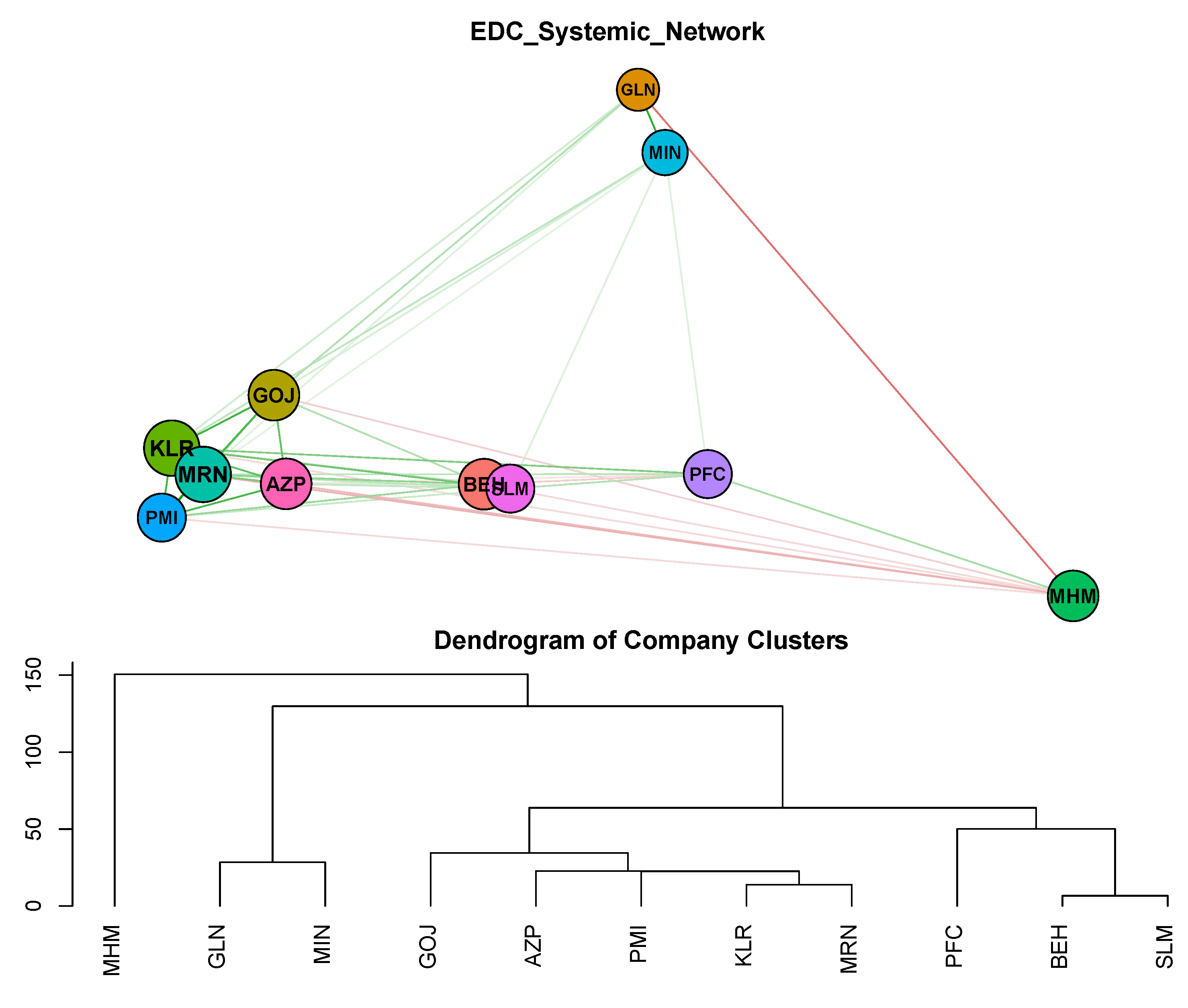
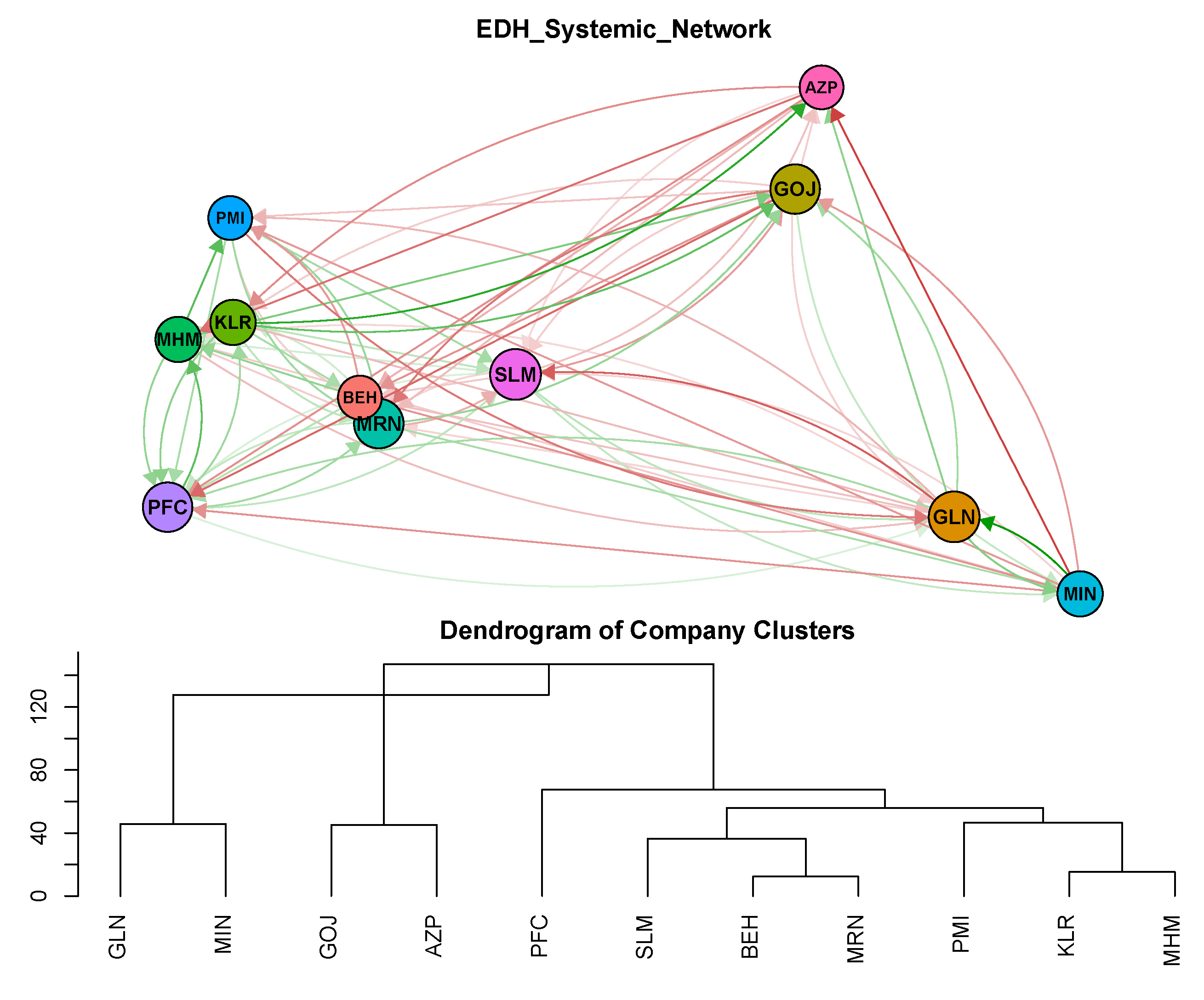
From a systemic perspective, Figure 3 reports the downside risk network among companies. The links are color-coded to describe the sign of reactions, where green (red) represents a positive (negative) reaction. The size of the vertices corresponds to the degree of the nodes. The companies are clustered according to median hierarchical clustering and summarized in dendrogram. The clustering of the companies in the figure reveal four community structures inherent in the full sample network. MHM alone constitutes one community, (GLN and MIN) constitute a second, (GOJ, AZP, PMI, KLR, and MRN) form the third, and the rest (PFC, BEH, and SLM) constitutes the fourth. These communities of companies seem to follow the pattern of correlation coefficient ranking shown in Table 3. More specifically, the negatively correlated stocks with the market index form a cluster, those with low-and-no correlation constitute two clusters, and the high-correlated ones form the fourth cluster.

To better understand the systemic importance of the companies,

Table 4. Centrality Measures for EDC network according to degree and eigenvector score from unweighted and weighted networks. Boldface values indicate the best choice for each metric.

	Degree		Eigenvector
	Unweighted	Weighted	Unweighted	Weighted
BEH	8	1.0527	0.3205	0.2408
GLN	5	0.5492	0.2015	0.1312
GOJ	8	1.9159	0.3064	0.3612
KLR	10	2.7267	0.3690	0.4354
MHM	8	−0.8734	0.3120	0.1759
MRN	10	2.1929	0.3690	0.4121
MIN	6	1.0105	0.2290	0.1140
PMI	7	2.2648	0.2890	0.4316
PFC	7	0.7739	0.2792	0.1676
SLM	7	1.3670	0.2766	0.2172
AZP	8	1.5752	0.3205	0.3597

summarize the EDC network using standard network measures. Since the EDC is an undirected network, the in-degree and out-degree of nodes are the same for weighted and unweighted networks. The same is true for hub and authority centrality measures. The table shows that if centrality is expressed by the number of connected counterparties (degrees), then the most important companies are KLR alongside MRN, followed by BEH, GOJ, MHM, and AZP. By weighting the connections among companies, KLR is ranked the most influential in terms of connectedness. Although MHM is highly interconnected with the rest, the associated weighted degree is −0.8734 since it is negatively correlated with almost all the others. If centrality, however, depends on the importance of an individual’s neighbor’s (i.e., eigenvector centrality), then the order of ranking of assets coincides with that of the degree.

In summary, both systematic and systemic EDC reveal a clustering behavior among the companies. Those who exhibit a high positive correlation with the market index have similar characteristics and are strongly interconnected among themselves. The companies identified in this group are (GOJ, AZP, PMI, KLR, and MRN). Companies of low-to-no correlation with the market index identified into two groups (GLN and MIN) and (PFC, BEH, and SLM). Lastly, MHM constituted a different cluster with a negative relationship with the market index and with almost all the other companies. The result, therefore, suggests that to hedge equity risk, MHM is the ideal choice of stock for investors. The most critical stock, highly correlated with the market and other food manufacturing companies is KLR.

3.2. Extreme Downside Hedging of Iran’s Food Industry

We compute the daily $CVaR$ as in (7) via a 30-day horizon rolling estimation of daily returns. As with every rolling window estimation, we acknowledge that by choosing a different and rather larger windows size might alter the daily estimates of the $CVaR$. We used the Monte Carlo sampling approach to draw 1000 samples of the loss vector given the mean and standard deviation of the loss distribution. We replicate the simulation 10 times to estimate the $CVaR$ series and the EDH model. We report the EDH results for a scenario model whose covariates include the market index and the other companies a single model.

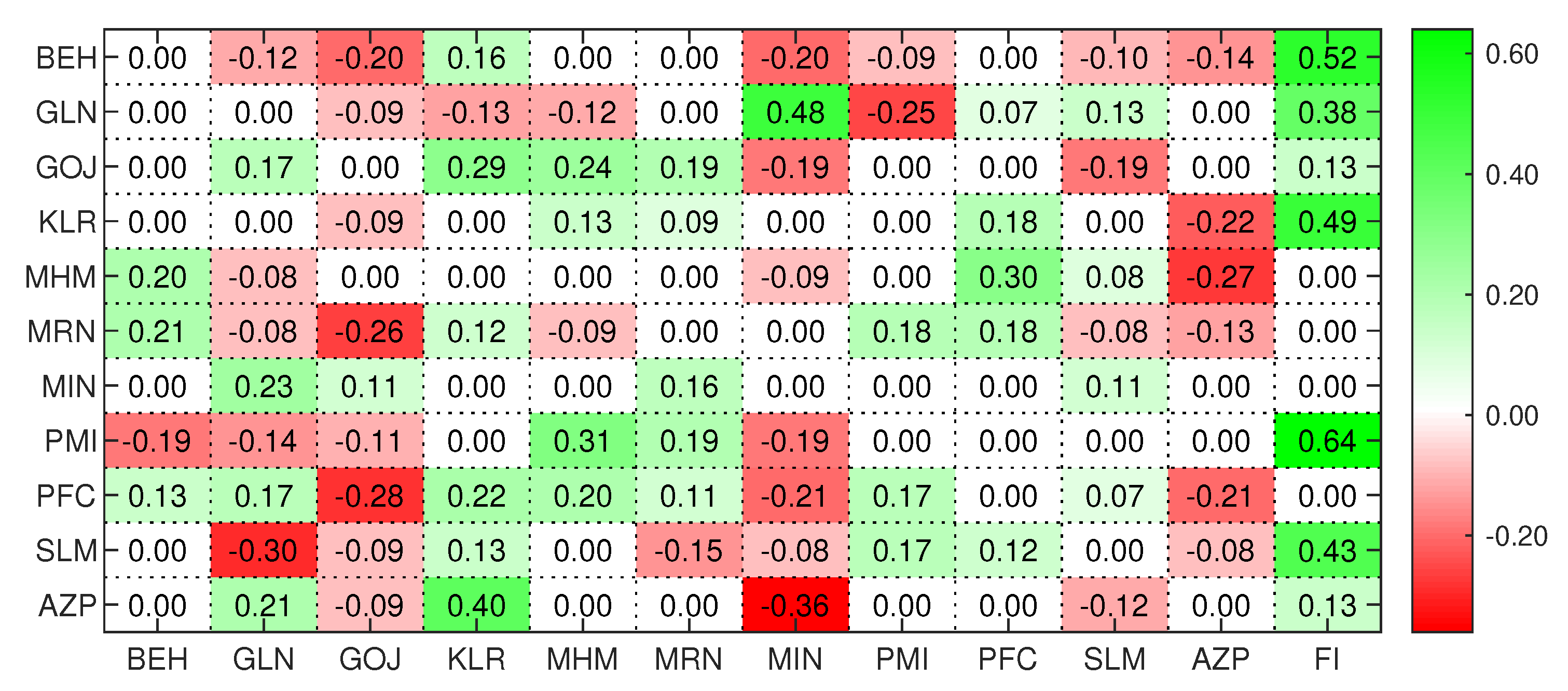
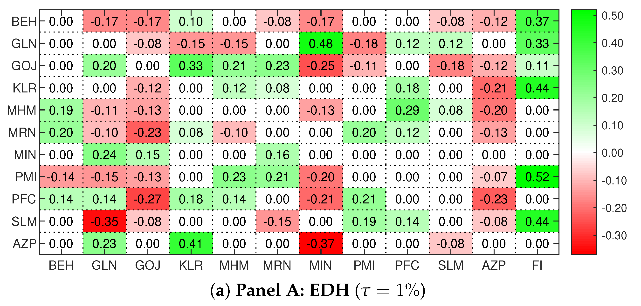
We begin by first discussing the results of the systematic analysis of the EDH which focuses on the relationship between the Food Industry index (FI) and the rest. This can be seen from the last column of Figure 4. This is followed by the systemic analysis, which concentrates on the results of Figure 4 without the last column.

3.2.1. Systematic EDH Analysis

Here the analysis is focused on how the stock return of the companies react to downside risk in the market index. A look at the last column of Figure 4 shows that most company returns reacts positively to turbulent events in the market. We rank the reactions of the companies according to the coefficients of the sensitivity and found three groups of companies. The outcome of the ranking exercise is reported in Figure 5. From the

Table 5. Ranking of companies based on systematic EDH coefficients. The light (dark) green color indicates weak (strong) positive reactions.

EDH Sensitivity	Companies
Strong	GLN,   SLM,   KLR,   BEH,   PMI
Mild	AZP,   GOJ
None	MHM,   MRN,   MIN,   PFC

, (GLN, SLM, KLR, BEH, PMI) constitute a group of assets that reacts strongly (or badly) in downturn market conditions. Companies like AZP and GOJ exhibit mild reactions, while (MHM, MRN, MIN, and PFC) have no reactions to turbulent market conditions. It is well known that assets that reacts mildly or have no reactions to downturn market events are often desirable and usually sell at a premium.

The result, therefore, suggests that based on the reaction of companies to downside movements in the Iran Food Industry over the past 5 years, it is worth selecting (AZP and/or GOJ) that have mild reactions to the market or choosing from (MHM, MRN, MIN, and PFC), which exhibit no sensitivity to extreme downturn market conditions.

Clearly, there seem to be some complementarity between the results of the EDH systematic outcome and that of the EDC. In particular, both results identify (PFC, MIN, and MHM) as instruments for diversification. Also, companies like (KLR, BEH, and PMI), which according to the EDC were highly correlated with the market, have strong reactions to extreme downside market risk.

3.2.2. Systemic EDH Analysis

We now turn our attention to analyze how the stock return of a company react to downside risk of other companies. A look at the columns of Figure 4 shows that the downside risk of AZP, GOJ, and MIN has negative effects on the returns of majority of other companies. PFC has only positive effects. The rest, however, have mixed interactions. In studying the rows of Figure 4, we notice that most of the companies have mild negative and positive reactions to the downsize risk of other companies.

Figure 5 display the network extracted from Figure 4 through the eigen-decomposition in (5). The result shows a scattered placement of the companies with some close communities like (GLN, MIN), (GOJ, AZP), (PFC), (SLM, BEH, MRN), and (PMI, KLR, and MHM).

The result of the most critical company to the transmission and receipt of risk is summarized in

Table 6. Centrality Measures for EDH systemic. Boldface values indicate the best choice for each metric.

	In-Degree	Out-Degree	Hub	Authority
BEH	6	4	0.1952	0.2917
GLN	7	9	0.3837	0.3003
GOJ	6	10	0.4164	0.2632
KLR	5	7	0.3149	0.1962
MHM	8	6	0.2541	0.3404
MRN	9	6	0.2349	0.3716
MIN	4	8	0.3466	0.1932
PMI	6	5	0.2493	0.2569
PFC	10	5	0.2176	0.4226
SLM	8	8	0.3418	0.3422
AZP	5	6	0.2756	0.2530

. Since the EDH is a directed network, we notice a difference in the in- and out-degrees. The hub and out-degree show GOJ as the most influential with 10 out-links, which indicates that GOJ is the top “transmitter” of risk in the sense that its downside risk influence the returns of all 10 remaining companies. It is closely followed by GLN. The authority and in-degree show PFC as the company whose return is highly sensitive to the downside risk of other companies. Thus, PFC is the highest “receiver” of risk, followed by MRN, SLM, and MHM.

3.3. Sensitivity Analysis

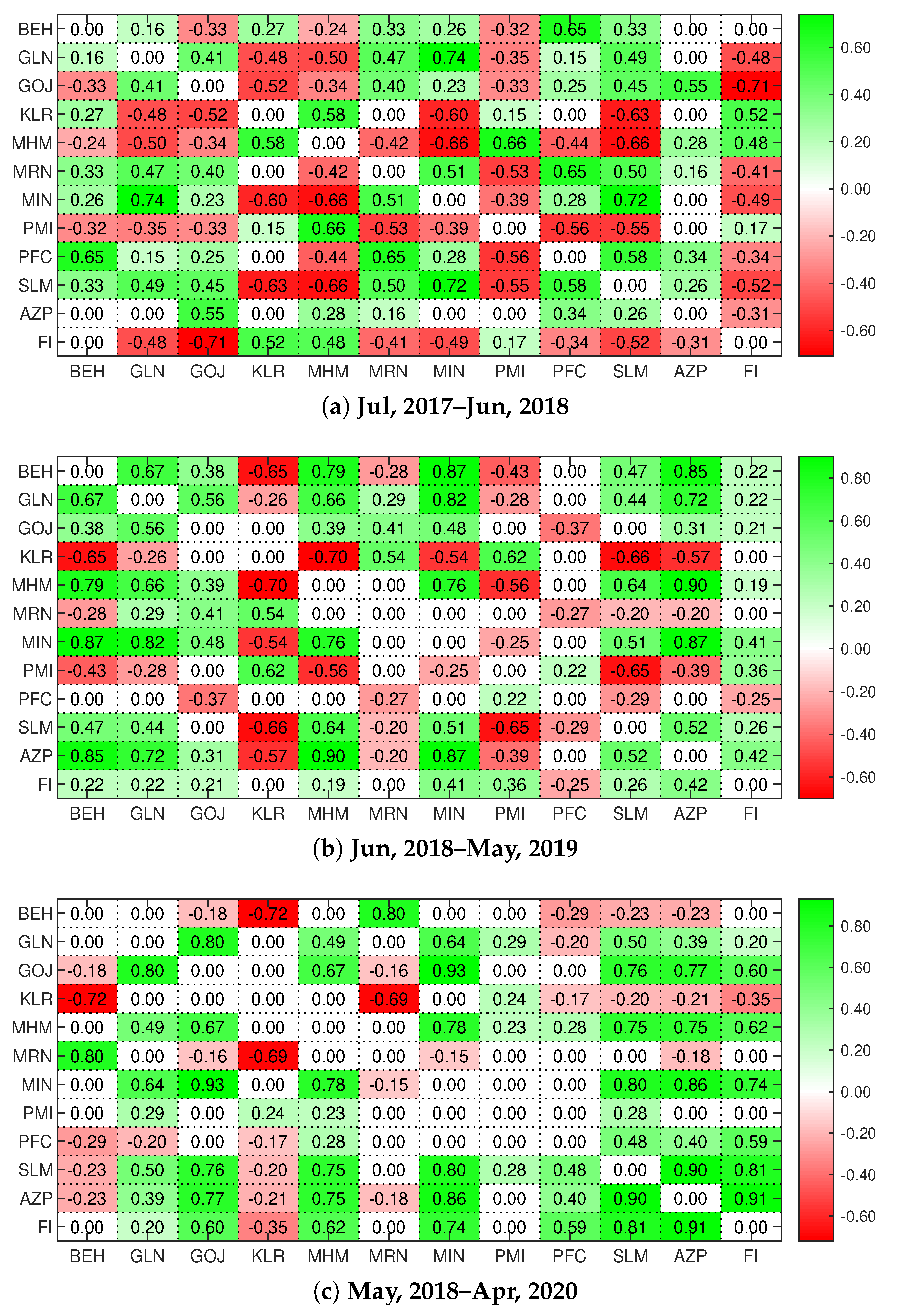
To validate the sensitivity of our empirical results, and our conclusions, we have conducted several robustness checks, as described by the following tables. The stability of the obtained results confirms the validity of our results. The result shows that the choice of different values of $\tau \in \{1\%,10\%\}$ does not change the results significantly (see Figure A1 and Figure A2). Figure A3 and Figure A4 refer, respectively, to EDC and EDH, calculated over three non-overlapping yearly periods. Both figures note the stability of the obtained results, which confirms the validity of our empirical findings.

4. Conclusions

In the paper, we extend the extreme risk model introduced by Harris et al. (2019) to analyze the systemic and systematic exposures of financial assets under severe firm-level and market conditions. The model is applied to study the interconnectedness among food manufacturing companies in Iran. We address the question of which company in the Iranian Food Industry is, from an investment viewpoint, the safest, or the most critical, and which companies transmit, or receive, risks from the market, particularly during crisis times.

Our result shows Mahram Manufacturing (MHM) as the safest and ideal stock to hedge equity risk due to its negative correlation with the market and other companies. This is in line with Hosseini et al. (2017), which shows that Mahram Manufacturing has the highest share in their portfolio selection. We found Glucosan Company (GLN) and Behshahr (BEH) Industries are the riskiest, with the lowest average return and the highest risk, whose returns reacts badly to downside market risk. The evidence shows that Gorji Biscuits (GOJ) and Pegah Fars Diary (PFC) as the main “transmitter” and “receiver” of downside risk.

In conclusion, our results show that the proposed extended downside risk measures are quite effective to individuate risky companies in the Iranian Food market. Future research will involve the application of the methodology to other markets and extension to portfolio optimization.