A Multi-State Approach to Modelling Intermediate Events and Multiple Mortgage Loan Outcomes


Abstract
1. Introduction
2. Literature Review
3. Modelling Intermediate Events and Multiple Loan Outcomes
3.1. Competing Risks
3.2. Multi-State Models
4. Statistical Analysis and Results
4.1. Data
4.2. Conceptual Framework
4.3. Results and Discussion
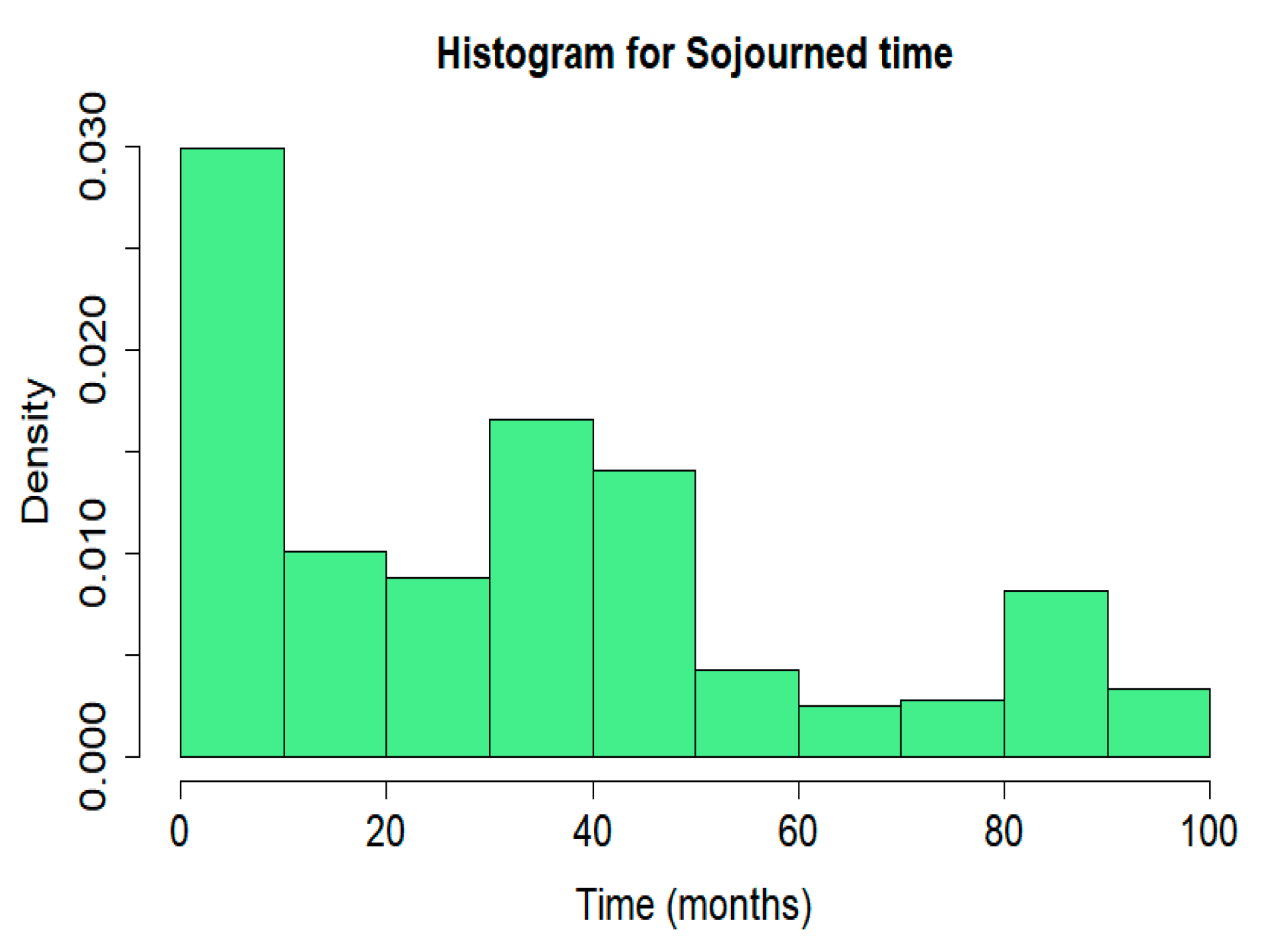
4.3.1. Descriptive Statistics
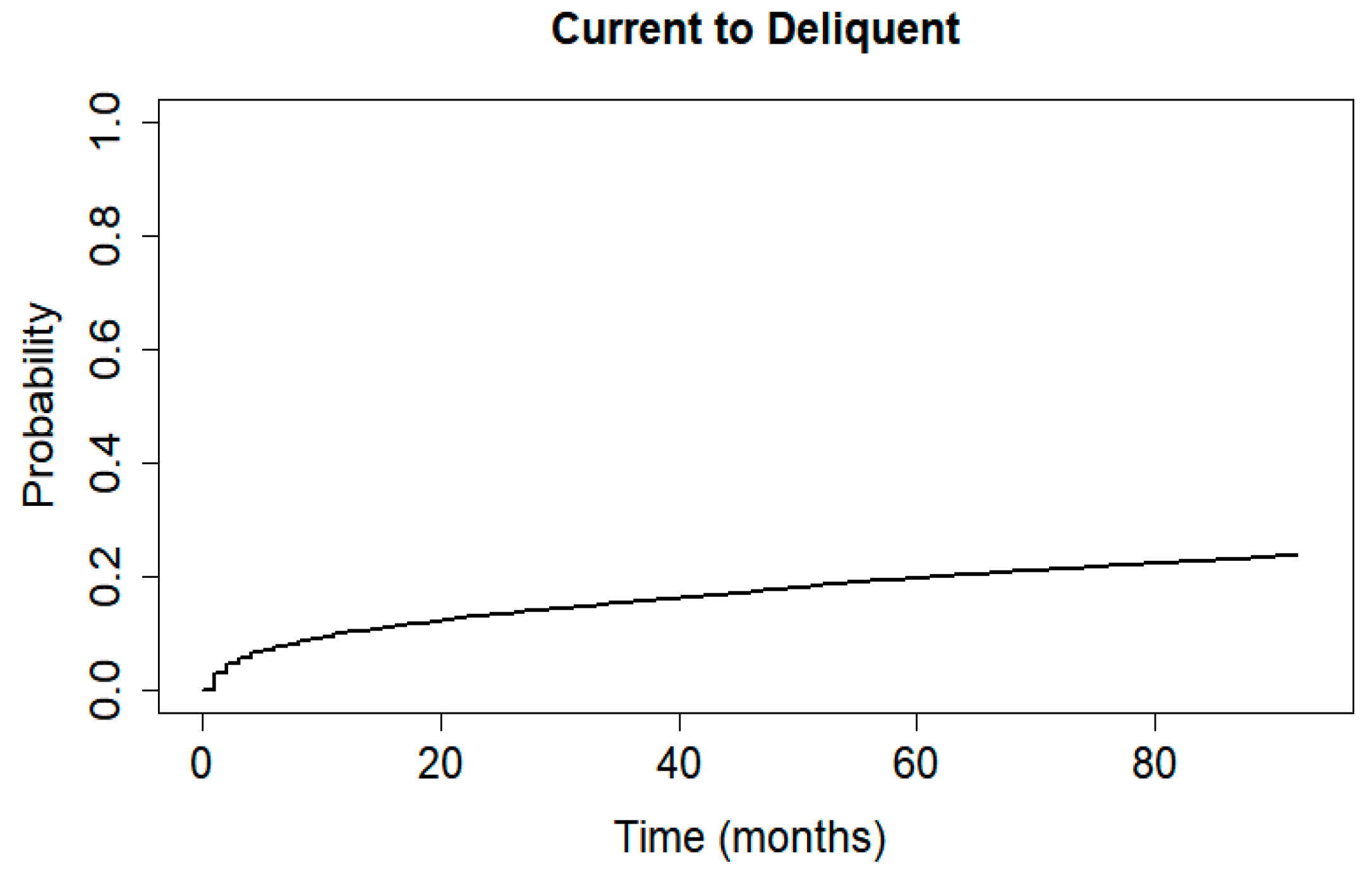
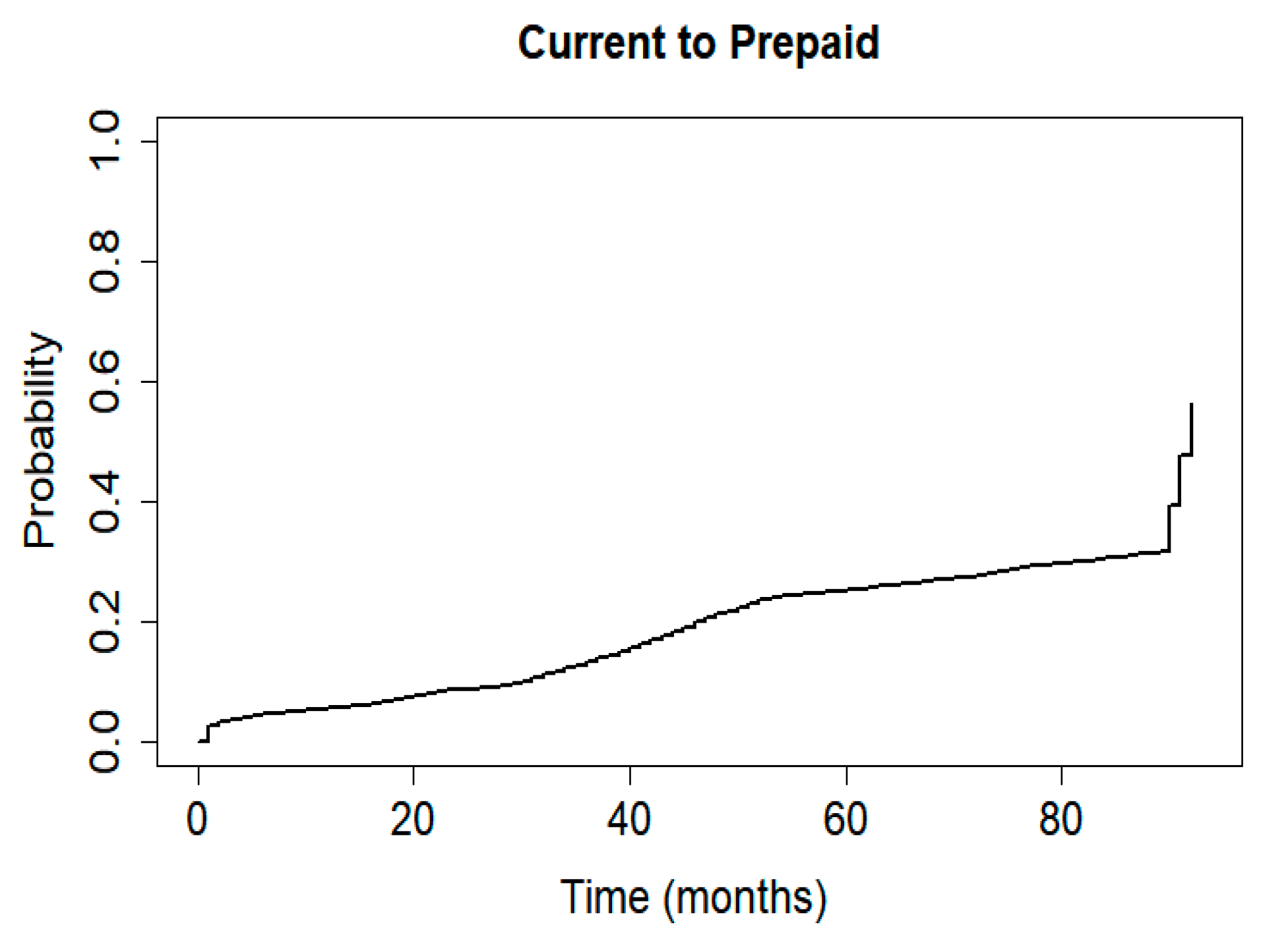
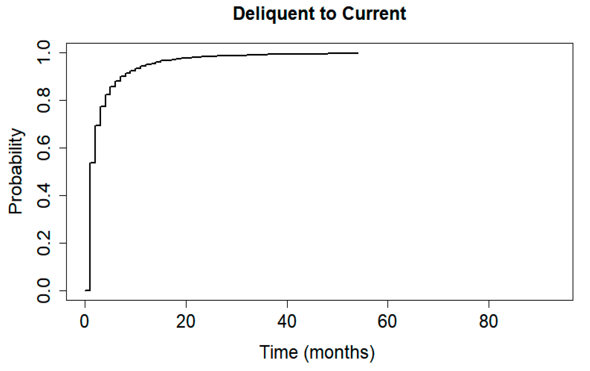
4.3.2. Transition Matrix
4.3.3. Cumulative Incidence Functions
4.3.4. Prognostic Factors for Event Specific Transitions
Current to Prepayment Transitions
Current to Delinquency and Default Transitions
Delinquent to Current Transition (Cure or Recovery)
Default to Current Transition (Cure or Recovery)
4.4. Model Validation
5. Conclusions
Author Contributions
Funding
Conflicts of Interest
References
- Altman, Edward I. 1968. Financial ratios, discriminant analysis and the prediction of corporate bankruptcy. Journal of Finance 23: 589–609. [Google Scholar] [CrossRef]
- Aalen, Odd O., and Søren Johansen. 1978. An empirical transition matrix for nonhomogeneous Markov chains based on censored observations. Scandinavian Journal of Statistics 5: 141–50. [Google Scholar]
- Abellán, Joaquín, and Javier G. Castellano. 2017. A comparative study on base classifiers in ensemble methods for credit scoring. Expert Systems with Applications 73: 1–10. [Google Scholar] [CrossRef]
- Agarwal, Sumit, Gene Amromin, Itzhak Ben-David, Souphala Chomsisengphet, Tomasz Piskorski, and Amit Seru. 2017. Policy Intervention in Debt Renegotiation: Evidence from Home Affordable Modification Program. Journal of Political Economy 125: 654–712. [Google Scholar] [CrossRef]
- Agarwal, Sumit, Gene Amromin, Souphala Chomsisengphet, Tim Landvoigt, Tomasz Piskorski, Amit Seru, and Vincent Yao. 2015. Mortgage Refinancing, Consumer Spending, and Competition: Evidence from the Home Affordable Refinancing Program. NBER Working Paper No. 21512. Cambridge: National Bureau of Economic Research. [Google Scholar]
- Ahlawat, Samit. 2018. Evaluation of Mortgage Default Characteristics Using Fannie Mae’s Loan Performance Data. Journal of Real Estate Finance & Economics 97: 58–69. [Google Scholar]
- Andersen, Per Kragh, and Niels Keiding. 2002. Multi-state models for event history analysis. Statistical Methods in Medical Research 11: 91–115. [Google Scholar] [CrossRef]
- Arminger, Gerhard, Daniel Enache, and Thorsten Bonne. 1997. Analyzing credit risk data: A comparison of logistic discrimination, classification tree analysis, and feedforward networks. Computational Statistics 12: 293–310. [Google Scholar]
- Aron, Janine, and John Muellbauer. 2010. Modelling and Forecasting UK Mortgage Arrears and Possessions. London: Department for Communities and Local Government. [Google Scholar]
- Aron, Janine, and John Muellbauer. 2016. Modelling and forecasting mortgage delinquency and foreclosure in the UK. Journal of Urban Economics 94: 32–53. [Google Scholar] [CrossRef]
- Baesens, Bart, Tony Van Gestel, Stijn Viaene, Maria Stepanova, Johan Suykens, and Jan Vanthienen. 2003. Benchmarking State-of-the-Art Classification Algorithms for Credit Scoring. The Journal of the Operational Research Society 54: 627–35. [Google Scholar] [CrossRef]
- Bajari, Patrick, Chenghuan Sean Chu, and Minjung Park. 2008. An Empirical Model of Subprime Mortgage Default from 2000 to 2007. NBER Working Paper 14625. Cambridge: National Bureau of Economic Research. [Google Scholar]
- Bajari, Patrick, Chenghuan Sean Chu, Denis Nekipelov, and Minjung Park. 2013. A Dynamic Model of Subprime Mortgage Default: Estimation and Policy Implications. Working Paper 18850. Cambridge: National Bureau of Economic Research. [Google Scholar]
- Bellotti, Tony, and Jonathan Crook. 2013. Forecasting and stress testing credit card default using dynamic models. International Journal of Forecasting 29: 563–74. [Google Scholar] [CrossRef]
- Beyersmann, Jan, Arthur Allignol, and Martin Schumacher. 2012. Competing Risks and Multi-State Models with R. New York: Dordrecht: Heidelberg: London: Springer. [Google Scholar]
- Black, Fischer, and Myron Scholes. 1973. The pricing of options and corporate liabilities. Journal of Political Economy 81: 637–54. [Google Scholar] [CrossRef]
- Bhutta, Neil, Jane Dokko, and Hui Shan. 2010. The Depth of Negative Equity and Mortgage Default Decisions. FEDS Series; Washington, DC: Board of Governors of the Federal Reserve System, pp. 2010–35. [Google Scholar]
- Bhutta, Neil, Jane Dokko, and Hui Shan. 2017. Consumer Ruthlessness and Mortgage Default during the 2007 to 2009 Housing Bust. The Journal of Finance 72: 2433–66. [Google Scholar] [CrossRef]
- Bravo, Jorge Miguel Ventura, and Carlos Manuel Pereira da Silva. 2006. Immunization Using a Stochastic Process Independent Multifactor Model: The Portuguese Experience. Journal of Banking and Finance 30: 133–56. [Google Scholar] [CrossRef]
- Butaru, Florentin, Qingqing Chen, Brian Clark, Sanmay Das, Andrew W. Lo, and Akhtar Siddique. 2016. Risk and risk management in the credit card industry. Journal of Banking and Finance 72: 218–39. [Google Scholar] [CrossRef]
- Campbell, John Y. 2013. Mortgage Market Design. Review of Finance 17: 1–33. [Google Scholar] [CrossRef]
- Carranza, Juan Esteban, and Dairo Estrada. 2013. Identifying the determinants of mortgage default in Colombia between 1997 and 2004. Annals of Finance 9: 501–18. [Google Scholar] [CrossRef]
- Castro, Vítor. 2013. Macroeconomic determinants of the credit risk in the banking system: The case of the GIPSI. Economic Modelling 31: 672–83. [Google Scholar] [CrossRef]
- Charlier, Erwin, and Arjan Van Bussel. 2003. Prepayment behavior of Dutch mortgages: An empirical analysis. Real Estate Economics 31: 165–204. [Google Scholar] [CrossRef]
- Chamboko, Richard, and Jorge M. Bravo. 2016. On the modelling of prognosis from delinquency to normal performance on retail consumer loans. Risk Management 18: 264–87. [Google Scholar] [CrossRef]
- Chamboko, Richard, and Jorge M. Bravo. 2019a. Frailty correlated default on retail consumer loans in Zimbabwe. International Journal of Applied Decision Sciences 12: 271–87. [Google Scholar] [CrossRef]
- Chamboko, Richard, and Jorge M. Bravo. 2019b. Modelling and forecasting recurrent recovery events on consumer loans. International Journal of Applied Decision Sciences 12: 257–70. [Google Scholar] [CrossRef]
- Chan, Sewin, Claudia Sharygin, Vicki Been, and Andrew Haughwout. 2014. Pathways After Default: What Happens to Distressed Mortgage Borrowers and Their Homes? Journal of Real Estate Finance and Economics 48: 342–79. [Google Scholar] [CrossRef]
- Crook, Jonathan N., David B. Edelman, and Lyn C. Thomas. 2007. Recent developments in consumer credit risk assessment. European Journal of Operational Research 183: 1447–65. [Google Scholar] [CrossRef]
- Danis, Michelle A., and Anthony Pennington-Cross. 2005. A Dynamic Look at Subprime Loan Performance. Journal of Fixed Income 15: 28–39. [Google Scholar] [CrossRef][Green Version]
- Deng, Yongheng, John M. Quigley, and Robert Van Order. 2000. Mortgage Terminations, Heterogeneity and the Exercise of Mortgage Options. Econometrica 68: 275–307. [Google Scholar] [CrossRef]
- Deng, Yongheng, John M. Quigley, Robert Van Order, and Freddie Mac. 1996. Mortgage default and low downpayment loans: The costs of public subsidy. Regional Science and Urban Economics 26: 263–85. [Google Scholar] [CrossRef]
- Di Maggio, Marco, Amir Kermani, Benjamin J. Keys, Tomasz Piskorski, Rodney Ramcharan, Amit Seru, and Vincent Yao. 2017. Interest Rate Pass-Through: Mortgage Rates, Household Consumption, and Voluntary Deleveraging. American Economic Review 107: 3550–88. [Google Scholar] [CrossRef]
- Du Jardin, Philippe, and Eric Séverin. 2011. Predicting corporate bankruptcy using a self-organizing map: An empirical study to improve the forecasting horizon of a financial failure model. Decision Support Systems 51: 701–11. [Google Scholar] [CrossRef]
- Elul, Ronel, Nicholas S. Souleles, Souphala Chomsisengphet, Dennis Glennon, and Robert Hunt. 2010. What “Triggers” Mortgage Default? The American Economic Review 100: 490–94. [Google Scholar] [CrossRef]
- Foote, Christopher L., Kristopher Gerardi, and Paul S. 2008. Negative equity and foreclosure: Theory and evidence. Journal of Urban Economics 64: 234–45. [Google Scholar] [CrossRef]
- Fuster, Andreas, and Paul S. Willen. 2017. Payment Size, Negative Equity, and Mortgage Default. American Economic Journal: Economic Policy 9: 167–91. [Google Scholar] [CrossRef]
- Gerardi, Kristopher, Adam Shapiro, and Paul Willen. 2007. Subprime Outcomes: Risky Mortgages, Homeownership and Foreclosure. Technical Report Working Paper 07–15. Atlanta: Federal Reserve Bank of Atlanta. [Google Scholar]
- Gerardi, Kristopher, Kyle Herkenhoff, Lee E. Ohanian, and Paul Willen. 2013. Unemployment, Negative Equity and Strategic Default. Working Papers Series; Atlanta: Federal Reserve Bank of Atlanta. [Google Scholar]
- Grimshaw, Scott D., and William P. Alexander. 2011. Markov chain models for delinquency: Transition matrix estimation and forecasting. Applied Stochastic Models in Business Industry 27: 267–79. [Google Scholar] [CrossRef]
- Guiso, Luigi, Paola Sapienza, and Luigi Zingales. 2009. Moral and Social Constraints to Strategic Default on Mortgages. NBER Working Paper No. 15145. Cambridge: National Bureau of Economic Research. [Google Scholar]
- Gupton, Gred M., Christopher Clemens Finger, and Mickey Bhatia. 1997. CreditMetricsTM–Technical Document. New York: JP Morgan, pp. 1–212. [Google Scholar]
- Guren, Adam M., Arvind Krishnamurthy, and Timothy J. McQuade. 2018. Mortgage Design in an Equilibrium Model of the Housing Market. NBER Working Paper 24446. Cambridge: National Bureau of Economic Research. [Google Scholar]
- Ha, Sung Ho. 2010. Behavioral assessment of recoverable credit of retailer’s customers. Information Sciences 180: 3703–17. [Google Scholar] [CrossRef]
- Ha, Sung Ho, and Ramayya Krishnan. 2012. Predicting repayment of the credit card debt. Computers and Operations Research 39: 765–73. [Google Scholar] [CrossRef]
- Hand, David J., and William E. Henley. 1997. Statistical Classification Methods in Consumer Credit Scoring: A Review. Journal of the Royal Statistical Society Series A (Statistics in Society) 160: 523–41. [Google Scholar] [CrossRef]
- Heagerty, Patrick J., Thomas Lumley, and Margaret S. Pepe. 2000. Time-dependent ROC curves for censored survival data and a diagnostic marker. Biometrics 56: 337–44. [Google Scholar] [CrossRef]
- Heagerty, Patrick J., and Yingye Zheng. 2005. Survival model predictive accuracy and ROC curves. Biometrics 61: 92–105. [Google Scholar] [CrossRef]
- Hosmer, W. David, Stanley Lemeshow, and X. Rodney Sturdivant. 2013. Applied Logistic Regression, 3rd ed. Wiley Series in Probability and Statistics; Hoboken: Wiley. [Google Scholar]
- Jones, Timothy, Dean Gatzlaff, and G. Stacy Sirmans. 2016. Housing Market Dynamics: Disequilibrium, Mortgage Default, and Reverse Mortgages. Journal of Real Estate Finance and Economics 53: 269–81. [Google Scholar] [CrossRef]
- Kaplan, Edward L., and Paul Meier. 1958. Nonparametric estimation from incomplete observations. Journal of the American Statistical Association 53: 457–81. [Google Scholar] [CrossRef]
- Kau, James B., Donald C. Keenan, Walter J. Muller, and James F. Epperson. 1992. A Generalized Valuation Model for Fixed-Rate Residential Mortgages. Journal of Money, Credit and Banking 24: 279–99. [Google Scholar] [CrossRef]
- Kau, James B., Donald C. Keenan, and Taewon Kim. 1993. Transaction costs, suboptimal termination and default probabilities. Real Estate Economics 21: 247–63. [Google Scholar] [CrossRef]
- Kelly, Robert, and Terence O’Malley. 2016. The good, the bad and the impaired: A credit risk model of the Irish mortgage market. Journal of Financial Stability 22: 1–9. [Google Scholar] [CrossRef]
- Kruppa, Jochen, Alexandra Schwarz, Gerhard Arminger, and Andreas Ziegler. 2013. Consumer credit risk: Individual probability estimates using machine learning. Expert Systems with Applications 40: 5125–31. [Google Scholar] [CrossRef]
- Lessmann, Stefan, Bart Baesens, Hsin-Vonn Seow, and Lyn C. Thomas. 2015. Benchmarking state-of-the-art classification algorithms for credit scoring: An update of research. European Journal of Operational Research 247: 124–36. [Google Scholar] [CrossRef]
- Liu, Bo, and Tien Foo Sing. 2018. “Cure” Effects and Mortgage Default: A Split Population Survival Time Model. Journal of Real Estate Finance and Economics 56: 217–51. [Google Scholar] [CrossRef]
- Mayer, Christopher, Karen Pence, and Shane M. Sherlund. 2009. The Rise in Mortgage Defaults. Journal of Economic Perspectives 23: 27–50. [Google Scholar] [CrossRef]
- Mayer, Christopher, Edward Morrison, Tomasz Piskorski, and Arpit Gupta. 2014. Mortgage modification and strategic behavior: Evidence from a legal settlement with Countrywide. American Economic Review 104: 2830–57. [Google Scholar] [CrossRef]
- McKinsey and Company. 1998. CreditPortfolioViewTM Approach Documentation and User’s Documentation. Zurich: McKinsey and Company. [Google Scholar]
- Mesnard, Benoit, A. Margerit, Cairen Power, and Marcel Magnus. 2016. Non-Performing Loans in the Banking Union: Stocktaking and Challenges. European Parliament, IPOL-EGOV. Available online: http://www.europarl.europa.eu/RegData/etudes/BRIE/2016/574400/IPOL_BRI(2016)574400_EN.pdf (accessed on 20 June 2019).
- Mian, Atif, Amir Sufi, and Francesco Trebbi. 2015. Foreclosures, House Prices, and the Real Economy. Journal of Finance 70: 2587–634. [Google Scholar] [CrossRef]
- Nyström, Kaj, and Jimmy Skoglund. 2006. A Credit Risk Model for Large Dimensional Portfolios with Application to Economic Capital. Journal of Banking & Finance 30: 2163–97. [Google Scholar]
- Noh, Hyun Ju, Tae Hyup Roh, and Ingoo Han. 2005. Prognostic personal credit risk model considering censored information. Expert Systems with Applications 28: 753–62. [Google Scholar] [CrossRef]
- Ncube, Mthuli, and Stephen E. Satchell. 1994. Modelling UK Mortgage Defaults Using a Hazard Approach Based on American Options. Working Paper 8. Cambridge: Department of Applied Economics, University of Cambridge. [Google Scholar]
- Ozkan, Mr F. Gulcin, and D. Filiz Unsal. 2012. Global Financial Crisis, Financial Contagion, and Emerging Markets. IMF Working Papers. Washington, DC: International Monetary Fund, vol. 12, p. 1. [Google Scholar]
- Piskorski, Tomasz, Amit Seru, and Vikrant Vig. 2010. Securitization and Distressed Loan Renegotiation: Evidence from the Subprime Mortgage Crisis. Journal of Financial Economics 97: 369–97. [Google Scholar] [CrossRef]
- Piskorski, Tomasz, and Amit Seru. 2018. Mortgage Market Design: Lessons from the Great Recession. Brookings Papers on Economic Activity, Economic Studies Program. Washington, DC: The Brookings Institution, vol. 49, pp. 429–513. [Google Scholar]
- Putter, Hein, Marta Fiocco, and Ronald B. Geskus. 2007. Tutorial in biostatistics: Competing risks and multi-state models. Statistics in Medicine 26: 2389–430. [Google Scholar] [CrossRef] [PubMed]
- Riddiough, Timothy J. 1991. Equilibrium Mortgage Default Pricing with Non-Optimal Borrower Behavior. Ph.D. dissertation, University of Wisconsin, Madison, WI, USA. [Google Scholar]
- Sarlija, Natasa, Mirta Bensic, and Marijana Zekic-Susac. 2009. Comparison procedure of predicting the time to default in behavioural scoring. Expert Systems with Applications 36: 8778–88. [Google Scholar] [CrossRef]
- Schwartz, Eduardo S., and Walter N. Torous. 1993. Mortgage Prepayment and Default Decisions: A Poisson Regression Approach. Real Estate Economics 21: 431–49. [Google Scholar] [CrossRef]
- Skoglund, Jimmy, and Wei Chen. 2016. The Application of Credit Risk Models to Macroeconomic Scenario Analysis and Stress Testing. Journal of Credit Risk 12: 1–45. [Google Scholar] [CrossRef]
- Stein, R. M., A. Das, Y. Ding, and S. Chinchalkar. 2010. Moody’s Mortgage Metrics Prime: A Quasi-Structural Model of Prime Mortgage Portfolio Losses. New York: Moody’s Research Labs. [Google Scholar]
- Stepanova, Maria, and Lyn Thomas. 2002. Survival analysis methods for personal loan data. Operations Research 50: 277–89. [Google Scholar] [CrossRef]
- Tian, Chao Yue, Roberto G. Quercia, and Sarah Riley. 2016. Unemployment as an Adverse Trigger Event for Mortgage Default. Journal of Real Estate Finance and Economics 52: 28–49. [Google Scholar] [CrossRef]
- Tong, Edward NC, Christophe Mues, and Lyn C. Thomas. 2012. Mixture cure models in credit scoring: If and when borrowers default. European Journal of Operational Research 218: 132–39. [Google Scholar] [CrossRef]
- Tracy, Joseph S., and Joshua Wright. 2016. Payment changes and default risk: The impact of refinancing on expected credit losses. Journal of Urban Economics 93: 60–70. [Google Scholar] [CrossRef]
- Vandell, Kerry D., Walter Barnes, David Hartzell, Dennis Kraft, and William Wendt. 1993. Commercial Mortgage Defaults: Proportional Hazards Estimation Using Individual Loan Histories. Real Estate Economics 21: 451–80. [Google Scholar] [CrossRef]
- Vandell, Kerry D. 1995. How ruthless is mortgage default? A review and synthesis of the evidence. Journal of Housing Research 6: 245–64. [Google Scholar]
- Volkov, Andrey, Dries F. Benoit, and Dirk Van den Poel. 2017. Incorporating sequential information in bankruptcy prediction with predictors based on Markov for discrimination. Decision Support Systems 98: 59–68. [Google Scholar] [CrossRef]
- Whelan, Karl. 2013. Ireland’s Economic Crisis: The Good, the Bad and the Ugly. UCD Working Paper. Dublin: University College Dublin. [Google Scholar]
| 1 | The recently approved BCBS (Basel IV) reforms of the standardised (CR-SA) approach (by making it more granular and risk sensitive) and of the CR-IRB approach for the calculation of risk weighted assets for credit risk will limit the extent to which banks can reduce capital requirements through the use of internal models (e.g., by eliminating the option to use any IRB approach for equity and advanced CR-IRB for institutions and large corporations). |
| 2 | The early repayment of a mortgage significantly impacts both the bank’s profitability, via reduced interest margins, the loss of foregone interest payments (less the risk of a default on the outstanding debt) and the bank’s interest rate and liquidity positions. Prepayment creates a reinvestment risk problem for banks that must be addressed by appropriate Asset–Liability Management (e.g., immunization) techniques (see, e.g., Bravo and Silva 2006). |


| Acquisition Variables | Description/Values |
|---|---|
| Loan Identifier | Mortgage loan unique identifier. |
| Origination Date | MM/YYYY |
| Loan Purpose | An indicator that denotes if a mortgage loan in a pool is either a purchase money mortgage or refinance mortgage. |
| Product Type | Fixed-rate mortgage or adjustable-rate mortgage. |
| Property Type | Single-Family (SF), Condo (CO), Co-Op (CP), Manufactured Housing (MH), PUD (PU) |
| Relocation Mortgage Indicator | Yes/No |
| Channel/ Origination Type | Retail (R), broker (B), correspondent (C) |
| Borrower Credit Score | 300–850 |
| Co-Borrower Credit Score | 300–850 |
| Debt-to-Income (DTI) Ratio | Calculated at origination and is obtained by dividing the borrower’s total monthly obligations by stable monthly income. |
| First-Time Homebuyer Indicator | Denotes if a borrower is a first-time homebuyer. |
| Number of Borrowers | Number of individuals who are obligated to repay the loan. |
| Number of Units | The number of units the mortgaged property has. |
| Occupancy Status | Indicates how the borrower used the mortgaged property at the time of origination. |
| Original Interest Rate | Mortgage original interest rate |
| Original Loan Term | The number of months for which a borrower’s payments are due |
| Original Loan-to-Value (LTV) | The Original LTV reflects the loan-to-value ratio of the loan amount secured by a mortgaged property on the origination date of the underlying mortgage loan. |
| Original Unpaid Principal Balance (UPB) | The original amount of the mortgage loan as indicated by the mortgage documents. |
| Performance Variables | Description/Values |
|---|---|
| Current Loan/Delinquency Status | The number of days (months) a borrower is delinquent, i.e., 0 = Current, or < 30 days overdue; 1 = 30–59 days; 2 = 60–89; 3 = 90–119; and so on. |
| Modification Flag | Y = Yes, N = No |
| Monthly Reporting Period | MM/DD/YYYY |
| Loan Age | Number of months after origination |
| Zero balance code | Reason mortgage loan’s balance was reduced to zero, e.g., 01= prepaid; 03 = Short Sale; and so on. |
| State | Description |
|---|---|
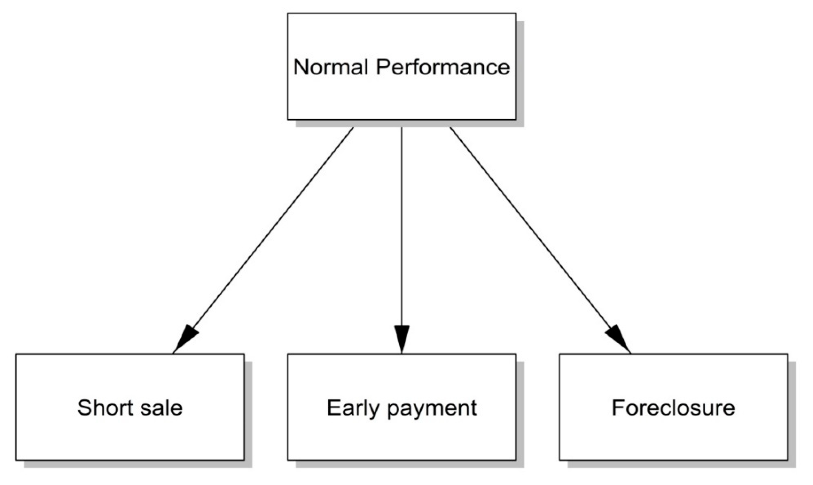
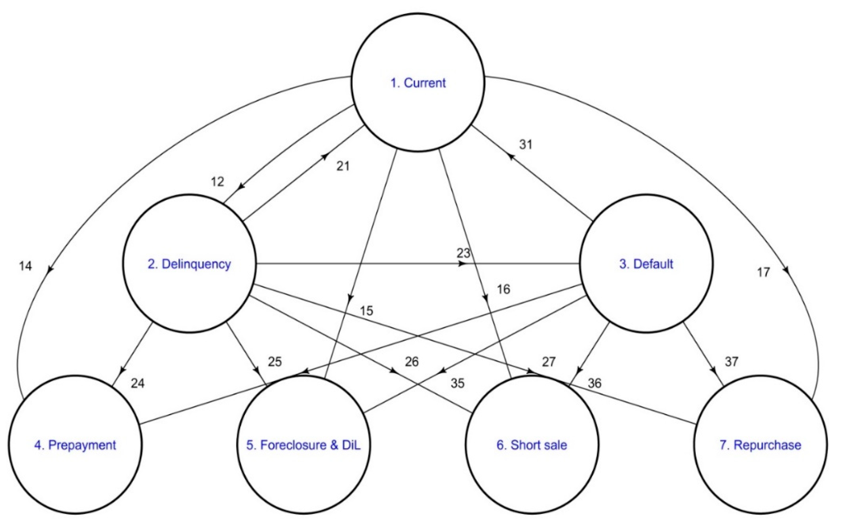
| Current/normal performance | This is when a borrower is up to date with payments or overdue by less than 30 days. |
| Delinquency | When payments are 30–59 days overdue. |
| Default | This is when a borrower missed payments for 60 days or more consecutively. |
| Prepayment | Occurs when a loan is paid in a shorter period than agreed contractually. |
| Mortgage foreclosure | Occurs when a borrower fails to pay in time or in full instalments and the lender repossesses the property. |
| Deed-in-Lieu, REO Disposition | This is when the borrower seeks release from the mortgage contract by voluntarily transferring the title of the property to the lender. |
| Short sale | This is when a homeowner sells a home for less than the balance remaining on a mortgage and pays off all (or a portion of) mortgage balance with the proceeds. |
| Recovery or cure | This is when a borrower once in delinquency or default resumes making payments. |
| Class of Variables | Variable | Category | Percent |
|---|---|---|---|
| Loan and borrower characteristics | Channel | Broker | 13.6 |
| Correspondent | 31.8 | ||
| Retail | 54.6 | ||
| First Time Homebuyer Indicator | Yes | 5.3 | |
| No | 94.7 | ||
| Property characteristics and purpose | Loan Purpose | Purchase | 15.3 |
| No Cash-out Refinance | 53.4 | ||
| Cash-out Refinance | 31.3 | ||
| Occupancy Status | Principal | 93.2 | |
| Second | 4.0 | ||
| Investor | 2.9 | ||
| Property Type | Condo | 6.8 | |
| Co-op | 0.4 | ||
| Manufactured Housing | 0.2 | ||
| Planned Urban Development | 19.5 | ||
| Single Family | 73.1 | ||
| Number of Units | 1 | 98.7 | |
| 2 | 1.1 | ||
| 3 | 0.1 | ||
| 4 | 0.1 | ||
| Behavioural variables | Relocation | Yes | 0.2 |
| No | 99.8 | ||
| Modification Flag | Yes | 0.3 | |
| No | 99.7 |
| Variable | Min | 1st Quantile | Median | Mean | 3rd Quartile | Max | Std Dev |
|---|---|---|---|---|---|---|---|
| Borrower characteristics | |||||||
| Borrowers’ Credit Score | 508.0 | 741.0 | 773.0 | 763.0 | 793.0 | 850.0 | 40.06 |
| Co-borrower’s Credit Score | 505.0 | 751.0 | 779.0 | 769.3 | 797.0 | 850.0 | 36.99 |
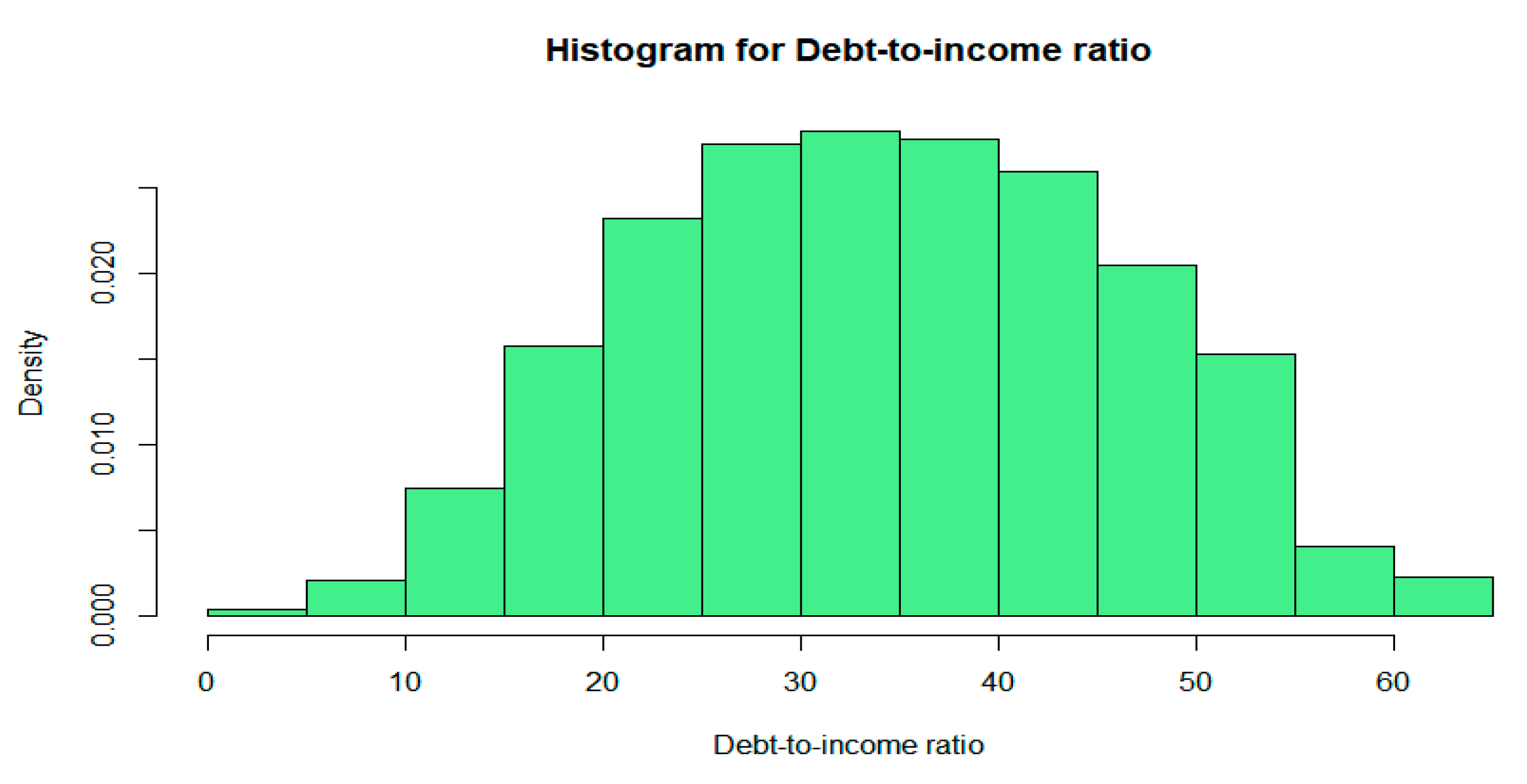
| Debt-to-Income Ratio | 1 | 24 | 32 | 33.08 | 42.0 | 64.0 | 11.81 |
| Number of Borrowers | 1.0 | 1.0 | 2.0 | 1.61 | 2.0 | 7.0 | 0.498 |
| Loan characteristics | |||||||
| Loan-to-Value | 3.0 | 60.0 | 73.0 | 68.77 | 80.0 | 97.0 | 15.65 |
| Original Loan Term (months) | 301 | 360 | 360 | 359.9 | 360 | 360 | 1.88 |
| Unpaid Principal Balance | 10,000 | 147,000 | 215,000 | 235,223.13 | 308,000 | 950,000 | 113,370.64 |
| Original Interest Rate | 1.88 | 4.75 | 4.875 | 4.98 | 5.125 | 8.625 | 0.361 |
| Behavioural variables | |||||||
| Loan Age at estimation (months) | 0 | 30 | 41.0 | 45.77 | 58.0 | 92.0 | 24.63 |
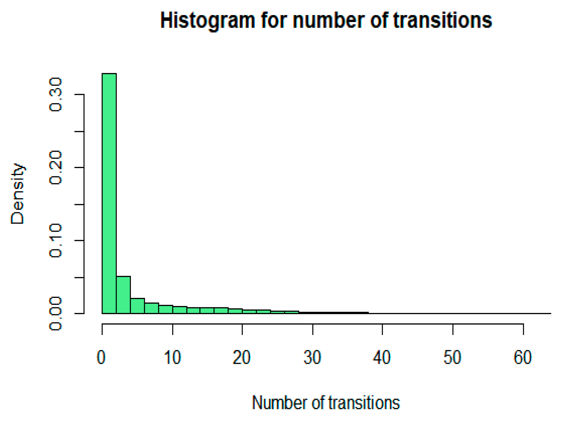
| Number of transitions | 0 | 1.0 | 1.0 | 1.27 | 1 | 63.0 | 2.156 |
| Sojourned time (months) | 1.0 | 26 | 40.0 | 43.61 | 54 | 92.0 | 25.96 |
| To | ||||||||
|---|---|---|---|---|---|---|---|---|
| Current | Delinquency | Default | Repurchase | Prepayment | Foreclosure and Dil | Short Sale | ||
| Current | 0.116 | 0.169 | 0.0 | 0.001 | 0.714 | 0.0 | 0.0 | |
| From | Delinquency | 0.706 | 0.0 | 0.271 | 0.0 | 0.023 | 0.0 | 0.0 |
| Default | 0.749 | 0.0 | 0.0 | 0.011 | 0.054 | 0.127 | 0.06 | |
| Current to Prepaid Transitions (1) | Current to Delinquent/Default (2) | Delinquent to Current (3) | Default to Current (4) | |
|---|---|---|---|---|
| Covariate | HR [Estimate] (SE) | HR [Estimate] (SE) | HR [Estimate] (SE) | HR [Estimate] (SE) |
| Modification Y | 2.37 [0.863 ***] (0.0145) | 5.57 [1.72 ***] (0.0299) | Omitted | Omitted |
| Purpose P | 0.979 [−0.0208 ***] 0.00778 | 0.819 [−0.199 ***] (0.0136) | 1.16 [0.152 ***] (0.0147) | 1.36 [0.305 ***] (0.0367) |
| Purpose R | 1.08 [0.08 ***] (0.00435 | 0.852 [−0.16 ***] (0.0136) | 1.06 [0.0564 ***] (0.00983) | 1.03 [0.0281] (0.0245) |
| Property Type CP | 0.78 [−0.249 ***] (0.0517) | 1.13 [0.123] (0.147) | 1.23 [0.207 ***] (0.0862) | 0.989 [−0.0112] (0.228) |
| Property Type MH | 0.654 [−0.424 ***] (0.0408) | 0.938 [−0.0636] (0.110) | 1.04 [0.0346] (0.0861) | 1.02 [0.0199] (0.223) |
| Property Type PU | 1.10 [0.0988 ***] (0.00111) | 0.993 [−0.00682] (0.0372) | 0.95 [0.0515 **] (0.0212) | 1.27 [0.236 ***] (0.0535) |
| Property Type SF | 1.12 [0.112 ***] (0.0104 | 1.21 [0.190 ***] (0.0343) | 0.927 [−0.0762 ***] (0.0188) | 1.27 [0.242 ***] (0.0417) |
| Relocation Y | 1.29 [0.253 ***] (0.0442) | 0.952 [−0.0495] (0.135) | 1.08 [0.0773] (0.106) | 1.83 [0.604 ***] (0.216) |
| Occupancy P | 1.49 [0.399 ***] (0.0128) | 1.10 [0.094 ***] (0.0335) | 0.818 [−0.201] (0.0216) | 1.04 [0.0404] (0.0573) |
| Occupancy S | 1.32 [0.274 ***] (0.0155) | 1.02 [0.0218] (0.0441) | 0.925 [−0.0783 **] (0.0491) | 1.01 [0.00872] (0.0832) |
| First time homebuyer U | 0.575 [−0.553 *] (0.2.36) | 0.92 [−0.11] (0.0113) | Omitted | Omitted |
| First time homebuyer Y | 0.901 [−0.104 ***] (0.0124) | 0.791 [−0.234 ***] (0.0355) | 0.985 [−0.0172] (0.0202) | 0.927 [−0.0753] (0.0475) |
| Units | 0.753 [−0.283 ***] (0.0143) | 0.854 [−0.1.58 ***] (0.0361) | 0.988 [−0.0116] (0.0216) | 0.828 [−0.189 ***] (0.0542) |
| Channel C | 1.03 [0.0267 ***] (0.00635) | 0.897 [−0.109 ***] (0.0192) | 0.978 [−0.0219 *] (0.0129) | 1.03 [0.0266] (0.0315) |
| Channel R | 0.911 [−0.0933 ***] (0.00587) | 0.785 [−0.242 ***] (0.0179) | 0.941 [−0.0861 ***] (0.0123) | 0.972 [−0.0284] (0.0303) |
| Co-borrower credit score | 0.998 [−0.00163 ***] (0.0000712) | 0.993 [−0.00714 ***] (0.000197) | Omitted | Omitted |
| Borrower credit score | 0.998 [−0.00174 ***] (0.0000706) | 0.989 [−0.0112 ***] (0.000199) | 1.0 1 [0.00202 ***] (0.0000895) | 1.03 [0.00174 ***] (0.000219) |
| DTI | 0.999 [−0.000439 *] (0.000175) | 1.02 [0.0214 ***] (0.000558) | 0.992 [−0.0081 ***] (0.00038) | 0.996 [−0.00415 ***] (0.000983) |
| Number of borrowers | 0.905 [−0.0999 ***] (0.0181) | 0.982 [−0.0186] (0.0518) | 1.04 [0.0378 ***] (0.00865) | 1.09 [0.0846 ***] (0.0219) |
| Loan-to-Value (LTV) | 0.996 [−0.00358 ***] (0.000128) | 1.01 [0.012 ***] (0.000462) | 0.994 (−0.0059 ***) (0.000317) | 0.991 [−0.0094 ***] (0.00147) |
| Loan term | 0.998 [−0.00234 *] (0.000977) | 1.03 [0.0294 ***] (0.00525) | 1.0 [0.000631] (0.00407) | 0.992 [−0.00842] (0.0091) |
| Original principal balance | 1.01 [0.0000019 ***] (0.0000000177) | 1.01 [6.62e−07 ***] (0.0000000589) | 1.0 [−0.000000001] (0.000000067) | 1.01 [−0.000001 ***] (0.000000018) |
| Original interest rate | 1.90 [0.644 ***] (0.00551) | 1.48 [0.39 ***] (0.048) | 0.868 [−0.141 ***] (0.00998) | 0.804 [−0.294 ***] (0.0401) |
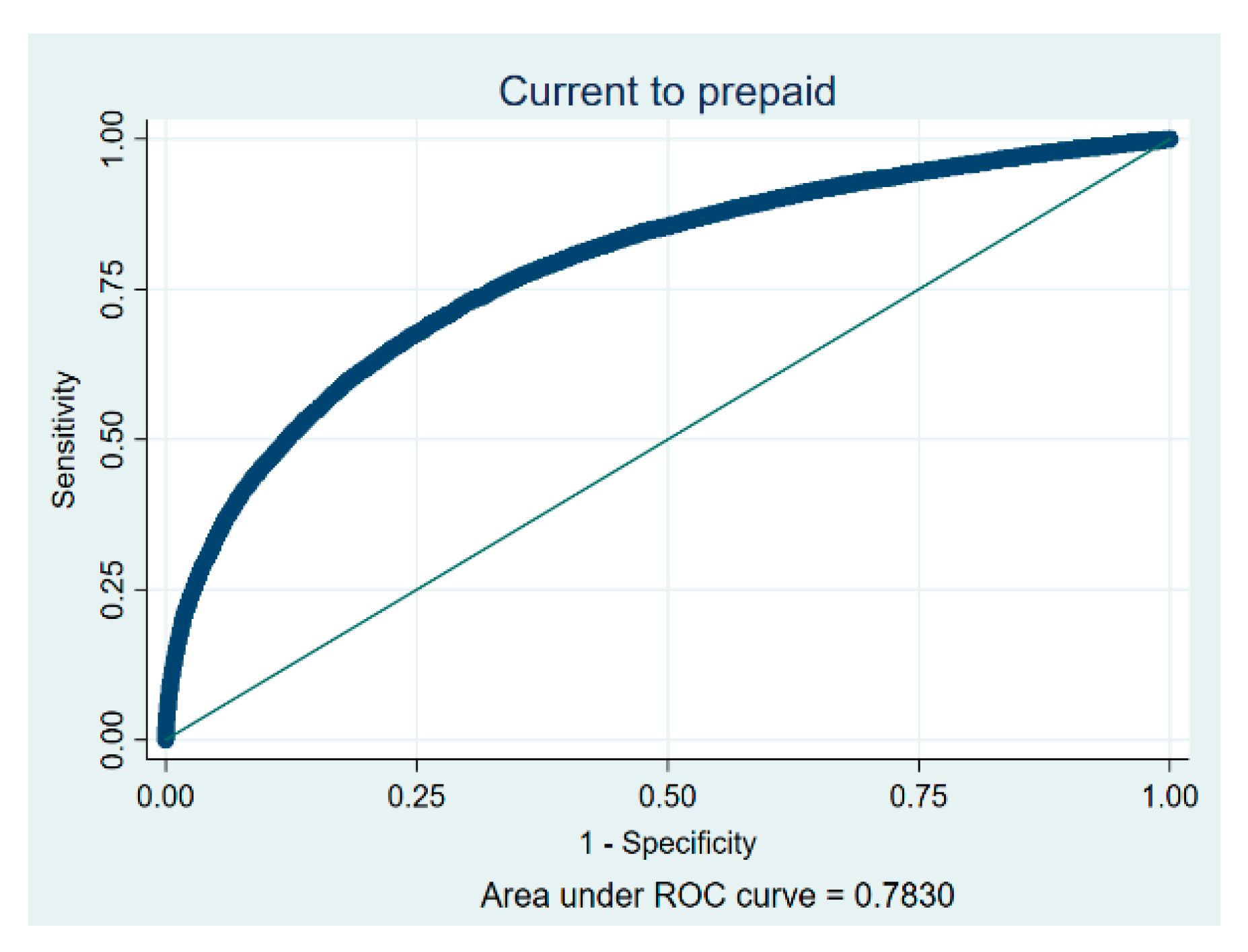
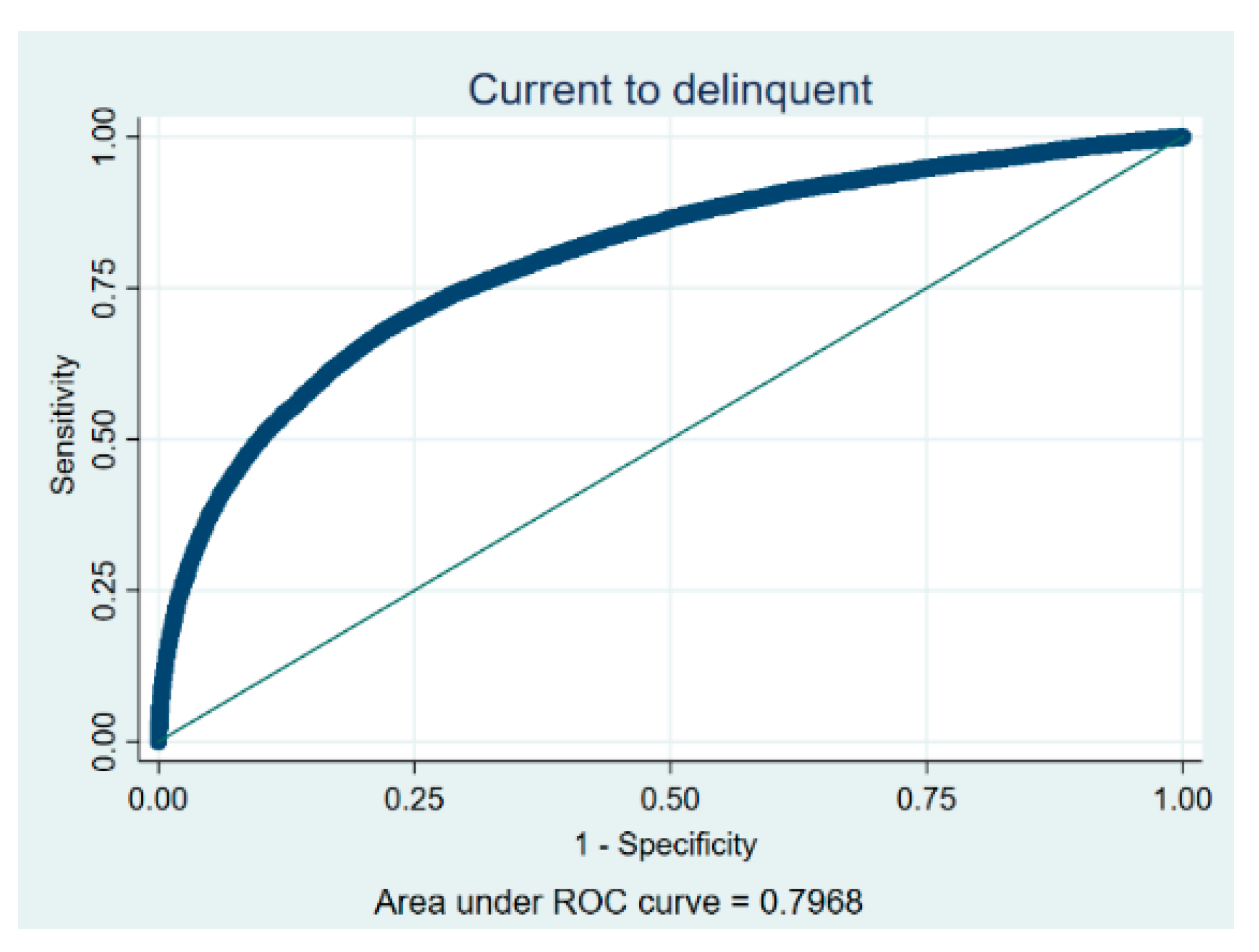
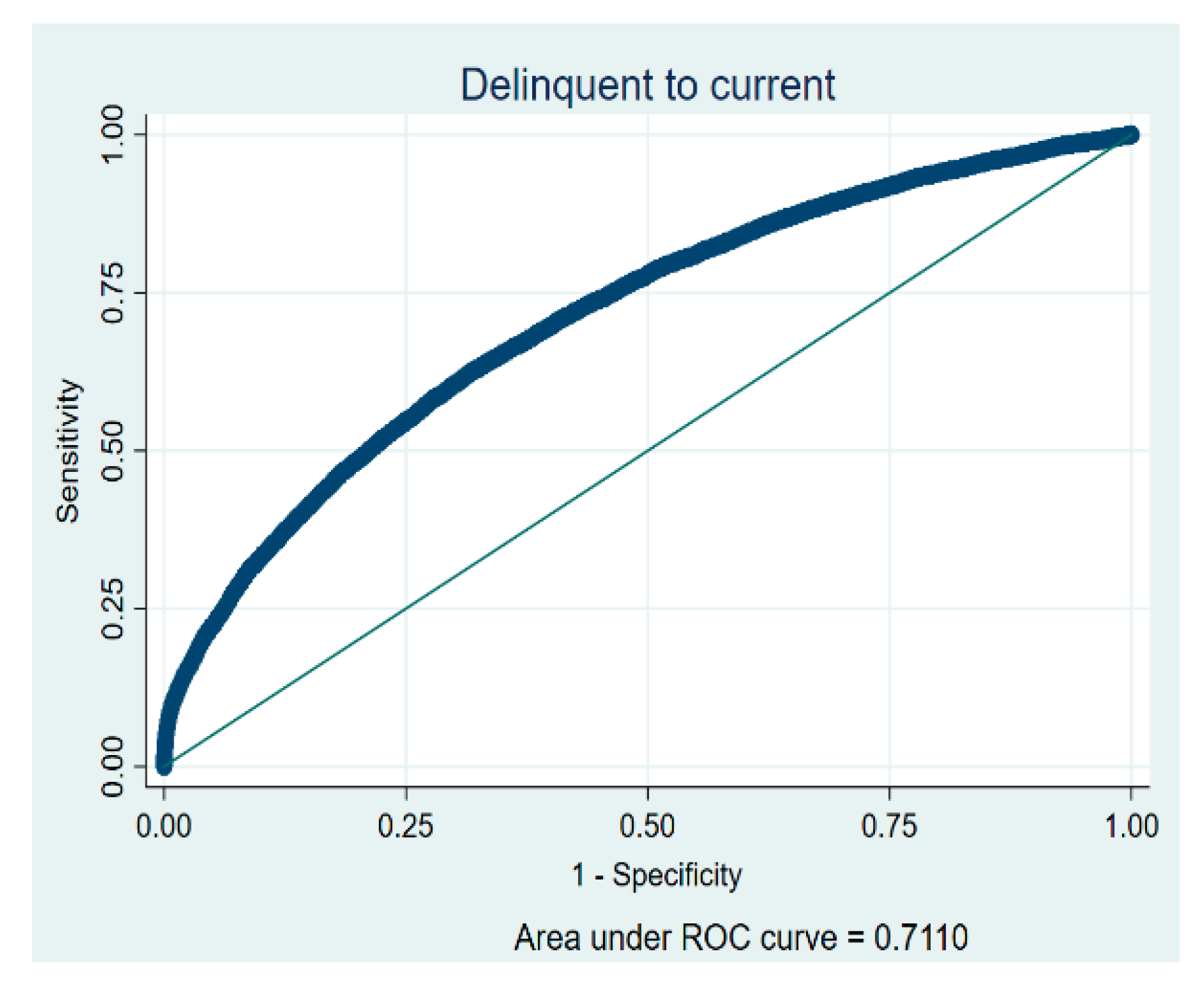
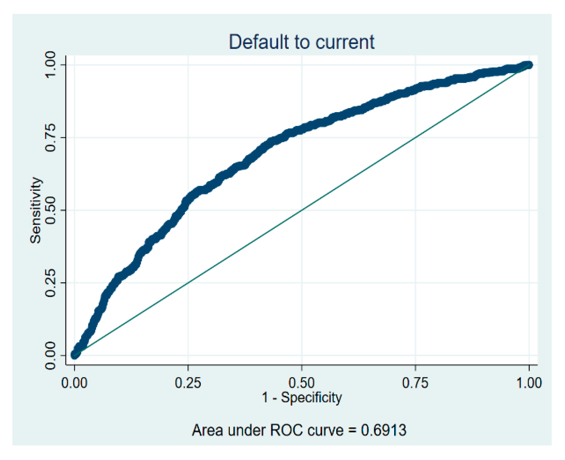
| Model | AUROC Curve | Standard Error | 95% Confidence Interval |
|---|---|---|---|
| Current to Prepaid | 0.7830 | 0.0021 | 0.77876–0.78718 |
| Current to Delinquent | 0.7968 | 0.0015 | 0.79380–0.79980 |
| Delinquent to Current | 0.6913 | 0.0083 | 0.68359–0.71604 |
| Default to Current | 0.7110 | 0.0024 | 0.70639–0.71569 |
© 2020 by the authors. Licensee MDPI, Basel, Switzerland. This article is an open access article distributed under the terms and conditions of the Creative Commons Attribution (CC BY) license (http://creativecommons.org/licenses/by/4.0/).
Share and Cite
Chamboko, R.; Bravo, J.M. A Multi-State Approach to Modelling Intermediate Events and Multiple Mortgage Loan Outcomes. Risks 2020, 8, 64. https://doi.org/10.3390/risks8020064
Chamboko R, Bravo JM. A Multi-State Approach to Modelling Intermediate Events and Multiple Mortgage Loan Outcomes. Risks. 2020; 8(2):64. https://doi.org/10.3390/risks8020064
Chicago/Turabian StyleChamboko, Richard, and Jorge Miguel Bravo. 2020. "A Multi-State Approach to Modelling Intermediate Events and Multiple Mortgage Loan Outcomes" Risks 8, no. 2: 64. https://doi.org/10.3390/risks8020064
APA StyleChamboko, R., & Bravo, J. M. (2020). A Multi-State Approach to Modelling Intermediate Events and Multiple Mortgage Loan Outcomes. Risks, 8(2), 64. https://doi.org/10.3390/risks8020064