1. Introduction
A loan is probably the most traditional banking product. However, when different people in different countries or even different people in the same country working in different customer segments speak about a loan, and they probably do not speak about the same product. The only common feature is that a lender gives money to a borrower and hopes to get back more than he has lent. Besides that, differences can be substantial. Critical drivers of product structure are the availability of funding and collateral. In some countries, only short-term funding is available to a bank. For this reason, interest rates of loans are rarely fixed over a long-term horizon but can be adjusted by a bank on short notice. In other countries, long-term funding is available, and loans are often fixed-rate or floating-rate loans, where the floating rate follows an objective rule like 6M Ibor plus a spread.
1 The most prominent type of loans that is linked to a particular collateral type is the mortgage. Here, often long maturities up to 30 years are observed. However, still, there are some differences between countries. For instance, in the US, a borrower can pass the key of a house to a bank when the house loses in value while in Germany defaulting on a mortgage is not that easy, and the borrower still is responsible for the residual amount between the loan balance and house value. There are a lot more differences. In some countries, borrowers have prepayment rights on their loans; in other countries, prepayment rights are less popular, but floating-rate loans are embedded with caps and floors. A lot more covenants can be included, like interest rates that increase with rating downgrades or minimum requirements on collateral value.
In this article, we develop a loan pricing scheme based on risk-adjusted return on capital (RAROC) as a performance measure. The purpose of this article is twofold. First, we propose a scheme that is directly implementable in banking practice drawing on input data that is readily available in most banks. This data consists of quotes from the interbank market, like deposit and swap rates, internal costs for funding and operation, and credit risk parameters related to borrower and collateral, i.e., statistical default probabilities and loss rates. We explicitly assume that no market information related to borrower credit quality, like bond or CDS spreads, is observable.
The proposed scheme is most valuable during loan origination where it provides a bank not only with the loan performance related to a particular offer of the loan’s interest rate but, in addition, with a decomposition of the interest rate into cost components associated with different bank operations related to lending. These are the funding of a bank loan by deposits, the management of loss risks, the hedging of interest rate risks, and the coverage of operational costs. Therefore, the scheme could be helpful in determining fund transfer prices between a bank’s operational units.
In addition, the scheme delivers a loan valuation. This could be valuable in price negotiations when loan portfolios are sold to investors. In economies with negative interest rate like the European Union, life insurers and pension funds are increasingly attracted by residential mortgages (
European Central Bank 2019) where they are still able to get a positive return in contrast to most government bonds. To determine a price during sales negotiations and for the investor’s ongoing reporting, our proposed model could be applied.
The second contribution of this article is an analysis of the RAROC scheme’s theoretical properties. Roughly speaking, RAROC is defined as (interest income − costs) / capital. On first glance this means if a bank would raise interest rates, leaving all other quantities unchanged, profitability would increase. However, it is intuitively clear that raising interest payments beyond the income of a borrower or the profit of a firm will lead to a default. This means, an economically meaningful performance measure should reflect this by having a low value in this scenario. We will show that, when properly relating borrower default probability and loan interest rate, this is indeed reflected by RAROC, i.e., that there is only a finite interval of interest rates where it is economically sensible for a bank to originate a loan. The market power of banks in a particular loan segment will then determine whether a bank can originate a loan at the lower or the upper end of this interval. This interval might be empty in cases where a borrower’s credit quality is too low, meaning that a bank should not originate a loan to this borrower regardless of the interest rate.
The general pricing framework presented in this article is not linked to a particular loan segment and is applicable both for corporate and retail lending. In the next Section, we will provide a literature review. In
Section 3, the loan pricing formula and its parameterization will be explained. In
Section 4, the RAROC pricing scheme will be developed, and the calculation of all its cost components will be derived. After that, in
Section 5 the theoretical properties of this scheme will be analyzed by linking the level of interest rates to the default rates of a borrower, and it will be shown how meaningful loan acceptance rules can be derived. In
Section 6, numerical examples are presented for illustration. The final Section concludes.
2. Literature Review
Our aim is developing a RAROC scheme that is applicable in banks world-wide drawing on inputs that are readily available in most banks. This is data related to internal costs and risk parameters measured statistically possible amended by expert judgment. As already outlined in the introduction, we explicitly assume that there is no market information of a borrower available, i.e., the borrower did not issue any bonds but all his debt consists exclusively of bank loans. This implies that the stream of literature using risk-neutral probabilities for asset pricing, e.g., as in
Jarrow et al. (
1997) or
Choi et al. (
2020), which are based on trading strategies in arbitrage-free markets, is not applicable in this context. A recent article on fair value approaches for loans is
Skoglund (
2017) where the utilization of market data for loan valuation is discussed. In most loan markets world-wide this is not feasible since the required market data is available only in countries with developed capital markets. Even in these countries, market valuations can only be applied to a small segment of the loan market, typically large corporates.
The RAROC concept dates back to the 70s, where it has been developed by practitioners. Often, it is applied in a one-period model analyzing one year only even if the loan maturity is longer (
Crouhy et al. 1999). The earliest extensions of RAROC to a multi-period framework are
Aguais et al. (
1998);
Aguais and Forest (
2000);
Aguais and Santomero (
1998). However, the description is very sketchy and loan pricing aspects that became important after the financial crisis are, of course, not included since these articles were written well before. Besides that, there is no split of the interest rate into cost components related to different operational units of a bank provided. Closing this gap is one purpose of this article.
When applying a RAROC scheme in practice, a number of aspects have to be considered that are not covered by our work but are required as inputs. These are the definition of capital for performance measurement, the allocation of total bank capital to sub-units, and the determination of target equity returns. As outlined in the introduction, RAROC is broadly defined as (interest income − costs)/capital. There are two definitions of capital, regulatory capital that is defined by supervisory rules
Basel Committee on Banking Supervision (
2006,
2011), and economic capital. Economic capital is measured by a credit portfolio model that should reflect economic reality more closely than the regulatory rules, e.g., by quantifying concentration risks. Most economic capital models are based on
Gupton et al. (
1997) and
CSFB (
1997). Once the loss distribution of a credit portfolio is computed a risk measure is derived. Usually expected shortfall is used to compute portfolio risk and the risk is distributed among the single credits in a process called capital allocation. For details see
Kalkbrener et al. (
2004);
Kalkbrener (
2005) and
Balog et al. (
2017). Both academia and practice have used predominantly economic capital models for performance measurement. A recent study is
Chun and Lejeune (
2020) where a multi-period model for loan pricing and profit maximization in an economic capital framework is developed. Compared to our work they do not model the interaction of default probabilities and interest rates but link the interest rate to a probability that a borrower accepts a loan offer. Besides that, their framework cannot be used for fund transfer pricing as they do not provide a loan’s cost components.
As pointed out by
Klaassen and Van Eeghen (
2018), economic capital usually exceeded regulatory capital in the past. For this reason, measuring loan performance by economic capital did not interfere with the regulatory rules since it was more conservative. However, this has changed with the recent Basel reforms resulting in higher minimum requirements of regulatory capital. When regulatory capital is higher than economic capital, performance measurement based on economic capital no longer works because it is overstating true performance. This motivated banks to move from economic to regulatory capital for performance measurement, as confirmed by a survey in (
Ita 2016, p. 38), and recent empirical research (
Akhtar et al. 2019;
Oino 2018). The RAROC scheme in this article does not depend on a particular capital definition and will work with either economic or regulatory capital. We will use regulatory capital for illustration and concrete examples because it is more tractable and increasingly more common in practice.
An important process where RAROC (or the related alternative RORAC) is applied, is the allocation of bank capital to business units. Here, a bank faces the problem that the managers of business units, who have only limited information about the total bank, should optimize the performance of their unit in a way leading to the maximum performance of the organization. The first article, demonstrating the usefulness of RAROC for this purpose is
Stoughton and Zechner (
2007). Extensions of this work are
Buch et al. (
2011);
Baule (
2014);
Turnbull (
2018) and
Kang and Poshakwale (
2019) where the latter even empirically demonstrate the usefulness of this approach. In this article, we do not analyze capital allocation on the business unit level but assume that this is done already. Instead, we focus on the loan-level and the costs and risks associated with each individual loan.
To evaluate loan performance, banks have to define a profitability target for their equity capital. This could be done by an application of the CAPM (Capital Asset Pricing Model). As pointed out by
Crouhy et al. (
1999) a uniform hurdle rate for all banking activities could lead to erroneously rejecting low-risk and accepting high-risk loans.
Miu et al. (
2016) propose a framework where target profitability can be defined on a granular basis for loan segments more accurately reflecting their riskiness. However, the application of their framework requires traded equity of borrowers, which limits its usefulness to a small part of the global loan markets. The determination of profitability targets is not part of this article. We assume this has been defined either quantitatively or by expert judgment, bank-wide or individually for loan segments. Since we focus on the individual loan, the scheme will work with either definition of profitability target.
Finally, we point out that we do not model the interaction of borrowers and lenders or the loan market as a whole. Modeling loan prices using equilibrium models is done, for instance, in
Greenbaum et al. (
1989);
Repullo and Suarez (
2004) and
Dewasurendra et al. (
2019). While these models shed some insights on the effect of regulatory rules on loan prices, they are of limited practical value as they miss out important aspects like loan structure or costs for interest rate risk management. An interesting example of modeling the borrower–lender interaction is
Zhang et al. (
2020) analyzing the special case of retailers loan decision in inventory financing under different bank loan offerings depending on the regulatory regime. In this article, we entirely focus on the bank and the costs associated with a loan. We will derive a set of interest rates under which it is profitable for a bank to offer a loan. Under what conditions or if at all a prospective borrower will accept an offer, is not part of this work.
3. Loan Pricing Formula
In this Section, the loan pricing formula and its parameterization are outlined. This formula builds the basis of the RAROC pricing scheme, which is explained in the next Section. Some aspects of the parameterization might not be apparent immediately but will be justified in the next Section. The value of a loan will be defined as the expected present value of all future cash flows. These are the interest rate payments, the amortization payments of the loan’s notional, and the liquidation proceeds of collateral in the case of a borrower default. The general expression for a loan’s value
V at time
t is given as
where
is the interest rate payment time in period
i,
,
is the year fraction of interest period
i,
the outstanding notional in each period,
the amortization payments,
the recovery rate in case of a default in period
i,
is the discount factor corresponding to time
, and
the survival probability of the borrower up to time
. It is assumed that default is recognized in payment times only and that the recovery rate summarizes the liquidation proceeds in case of default discounted back to default time.
The quantities
,
, and
are defined by the loan terms. The amortization payments depend on the loan structure, i.e., whether the loan is a bullet loan, an installment loan or an annuity loan. The interest rate
could be fixed or floating. In the case of a fixed-rate loan, the interest rate in each period is
y, where we assume that
y is fixed and period-independent. In the case of a floating-rate loan, the interest rate is
, where
is an Ibor rate, which is fixed at the beginning of each interest rate period
i and
s is a spread that is assumed constant throughout the loan’s lifetime. We will use the notation
for the interest rate in period
i with
where
is the forward rate corresponding to the floating rate
. To compute forward rates a second discount curve is needed, which will be denoted with
. Forward rates are computed as
It remains to explain how the parameters discount factors, survival probabilities, and recovery rates are determined. This is done in a separate subsection for each parameter.
3.1. Discount Factors
The pricing Formula (
1) requires two discount curves, the discount curve for discounting cash flows and the forward curve for computing forward rates for floating-rate loans. The forward curve is computed from the money market and the swap market. Usually, the forward curve up to one year is computed from deposit rates and forward rate agreements. Swap rates exist for maturities from one year up to 30 years in some currencies. A swap rate
is the fixed-rate of a swap, which periodically exchanges the fixed-rate with a Ibor rate
with tenor
. If the loan is linked to the same Ibor rate the discount factors
can be computed from the relation
where
is the start date of the swap,
are the payment times of the fixed leg and
are the day count fractions of the fixed leg. Usually, a bootstrap algorithm is applied in computing
starting from the swap rate with the lowest maturity and moving forward in swap maturities iteratively using the results of the previous calculation to compute the discount factors corresponding to higher maturities.
If the loan is linked to a different Ibor rate
with tenor
, the above curve cannot be used for computing forward rates. The spread of a basis swap exchanging periodically Ibor payments with tenor
for Ibor payments with tenor
has to be added to
before the bootstrapping starts. We assume the basis swap exchanges
for
, where
is the basis swap spread which depends on the maturity of the basis swap and can be negative.
2 This changes Equation (
4) to
The discount curve
has to reflect the funding conditions of a bank. It is computed from the fund transfer prices that are provided by a bank’s treasury. Typically fund transfer prices are given for a grid of standardized tenors like, 1Y, 2Y,
…, 10Y and are provided as Ibor + spread. This means, that internally the credit department buys a bond from the treasury department with a notional equal to the amount they intend to lend to a borrower. The coupon of this funding instrument is linked to a Ibor rate
with tenor
plus a spread
depending on a loan’s maturity. The discount curve
can be computed from the relation
where
are interest rate payment times of the funding bond and
are the year fractions of the interest rate periods. The forward rates
are computed by (
3) using the swap curve linked to
. For the calculation of discount factors, the notional is normalized to 1. Similar to the bootstrapping of the swap curve, a bootstrapping of the funding curve can be performed starting from the lowest maturity and working iteratively up to the highest. If a loan has a fixed rate of interest or a floating rate linked to the Ibor rate
we get the discount factors in (
1) as
.
If the loan’s interest rate is floating and its Ibor’s tenor
again an adjustment by basis swap spreads is needed. Assume that the basis swap for
and
exchanges
for
where again
might be negative. Equation (
6) has to be adjusted to
where the payment times and year fractions in (
7) are the same as for the loan. Forward rates
are computed from the swap curve corresponding to the Ibor rate
. Bootstrapping this relation results in the discount curve needed for discounting a loan’s cash flows. Why this is a sensible discount curve for cash flow discounting will become clear in
Section 4.
3.2. Survival Probabilities
Equivalent to the calculation of a survival probability up to time T is the calculation of a default probability . Default probabilities with a time horizon of one year are typically one outcome of a bank’s rating system. We assume that a bank’s rating system has n grades where the n-th grade is the default grade. Again, remember that one key assumption of this article was the absence of market information like bond or CDS spread. Therefore, a bank has to rely on statistical information which is derived using balance sheet information for corporate clients, personal information of retail clients, and expert judgment as inputs. There are typically two ways of how banks could extract statistical information about defaults from their rating systems to estimate multi-year default probabilities.
In the first approach, a one-year transition matrix is estimated from the rating transitions that are observed in a bank’s rating system. The resulting matrix is denoted with . The entries of the matrix are denoted with where is the probability that a borrower in rating grade k moves to grade l within one year. The matrix has the following properties:
The entries of are nonnegative, i.e., , .
All rows of sum to one, i.e., , .
The last column , contains the one-year default probabilities of the rating grades .
The default state is absorbing, i.e., , and .
If we assume that rating transitions are Markovian, i.e., they depend on a borrower’s current rating grade only, and that transition probabilities are time-homogeneous, i.e., the probability of a rating transition between two-time points depends on the length of the time interval only, then it is possible to apply the theory of Markov chains to construct transition matrices
for an arbitrary full-year
h just by multiplying
with itself:
Once is computed, the default probability can be read from the last column in the k-th row. Interpolating the values gives the term-structure of default probabilities for rating grade k.
In the second approach, banks directly estimate a term-structure of default probabilities, i.e., for each rating grade
k a function
is estimated where
is the probability that a borrower in rating grade
k will default within the next
T years. From the term structure of default probabilities given today, conditional default probabilities for future times
U can be computed easily. The probability
that a borrower in rating grade
k will default up to time
T conditional that he is alive at time
U is given by
One way of estimating
is by using techniques from survival analysis, where the Cox proportional hazard model has been successfully applied in a credit risk context by numerous authors. Examples are
Banasik et al. (
1999) and
Malik and Thomas (
2010). In this model,
is parameterized as
where
are model coefficients,
borrower-dependent risk factors like balance sheet ratios for companies or personal data for retails clients and
a borrower-independent baseline hazard function. Borrowers with similar
can be summarized into a rating category
k and are then represented by the curve
.
Throughout this article, we will assume that
is estimated by a Cox proportional hazard model as in (
10). However, this is by no means the only way to estimate a default probability (PD) term-structure. A good overview of available methodologies is provided in
Crook and Bellotti (
2010).
3.3. Recovery Rates
Recovery rates reflect the degree of collateralization of a loan. They can be period-dependent. For instance, if a loan is amortizing and the collateral value stays the same over a loan’s lifetime, a loan becomes less risky over the years. This should be reflected in an increasing recovery rate. One pragmatic way to include collateral in a loan pricing framework is to provide the collateral value as input. This collateral value should not be the current market value of collateral but include the loss given default (LGD) of the collateral, i.e., the expected loss in value in the case of a borrower default. This loss can stem from price reductions in a distressed sale or reflect the costs of a liquidation process, e.g., for lawyers. Overall, the collateral valuation and LGD estimation process is complex and beyond the scope of this article. Some ideas can be found in articles on LGD estimation in
Engelmann and Rauhmeier (
2006).
For the purpose of loan pricing, we assume that such a process exists and that the outcome is a collateral cash value
C. For the unsecured part of a loan, a bank estimates a recovery rate
. From these data, the recovery rate
in each period is computed as
In (
11) a cap of 100% was introduced. It depends on the specific legal environment of a country’s loan market, whether recovery rates of more than 100% are possible or not. In case recovery rates can be larger than 100%, this assumption can be relaxed.
Note, that when applying this approach, consistency is an important issue. In (
11) the recovery rate is related to the outstanding notional. In internal risk parameter estimation processes, recovery rates (or, equivalently, LGD values) are often estimated with respect to outstanding notional plus one interest payment. Since loan pricing and risk parameter estimation is usually done in different departments of a bank, one has to take some care to ensure that consistent definitions and assumptions are used throughout a bank. Where this is not the case, appropriate transformations have to be defined.
4. RAROC Scheme
The main purpose of this Section is the derivation of a RAROC scheme for calculating the interest rate of a loan which covers all costs and adequately compensates for the risks associated with a loan. For bank internal purposes, it is important to split the interest rate into its components, i.e., which part of the interest rate reflects funding costs, which part expected losses, or which part basis swap hedging costs. For this reason, a RAROC scheme is derived step-by-step using the general valuation Formula (
1). Before we start, we have to make an assumption on the disbursement of a loan’s notional. This is not reflected in the valuation equation (
1). The assumption in this article is that a loan’s notional is disbursed on disbursement dates
and that on the date
the amount
is paid out to the borrower. The total notional
is the sum over all disbursements
.
The first component of the proposed RAROC scheme is the base swap rate. It is only relevant for a fixed-rate loan. For a floating-rate loan, this component is zero. The base swap rate is the fixed-rate that has to be charged by a bank that leads to an identical present value as the stream of Ibor payments. This rate is needed as a reference point to make floating-rate and fixed-rate loans comparable. The base swap rate
at valuation time
t is computed from
Alternatively,
can be interpreted as the interest rate that has to be charged for fixed-rate loans to make assets equal to liabilities in a bank’s balance sheet under the assumption that all other costs and risks can be ignored. Using this as a starting point, we will add all other relevant cost components of a loan to
in the following steps. To simplify the notation, we will use the abbreviation
This is the sum of all parts of the total loan balance that are already paid out at time t and the present value of the loan parts that still have to be disbursed.
In the next step, funding costs are computed. This is a bit awkward because funding might be linked to a Ibor tenor that is different from the payment frequency of the loan. To separate funding costs from basis swap hedging costs, we have to use the discount curve
and, if the loan is a floating rate loan, compute forward rates from the swap curve corresponding to the Ibor rate
. For a floating-rate loan, this leads to the condition
where
are the payment times of the funding bonds in (
6),
is the average notional in an interest rate period and
is the spread over Ibor that has to be paid by a borrower to cover funding costs. To give an example for clarification, suppose
6M and
1M. Since a loan might be amortizing, in each 6M period, the notional might change from month to month. Assuming that a repayment of the notional immediately leads to a reduction in the outstanding bonds for funding, the interest paid on the funding bonds has to be reduced with the amortizations. The mismatch in interest tenors is reflected in the averaging of the loan’s outstanding notional. If the mismatch is the other way round, i.e.,
, this problem does not exist. Solving (
14) for
gives
where we used the abbreviations
and
. For a fixed-rate loan, the solution can be derived from (
15) by setting all forward rates
to zero and replacing
by the fixed-rate
. After solving for
the funding cost margin
can be computed as
.
When the payment frequencies of funding bonds
and the loan
are different, a basis swap is needed for hedging the mismatch in Ibor payments. These hedging costs can be computed from (
14) by replacing the discount curve
with the loan’s discount curve
and going back to the loan’s payment frequency. This leads to
where
is the interest margin covering both funding and swap costs. Solving (
16) leads to
from which the margin for hedging costs
can be computed as
. Again, the case of a fixed-rate loan is covered by setting
and replacing
by the fixed rate
. The margin
associated with basis swap costs is computed as
.
So far, we have considered cost components that are independent of a loan’s default risk. The next step is taking default risk into account. To derive a margin
reflecting expected loss risk, the condition expected assets equals liabilities is applied. We use the abbreviations
and
In (
19), the survival probabilities reflect the fact that a bank will only pay out future tranches of a loan when the borrower is still alive. Using these abbreviations and (
1), the interest rate spread
containing expected loss risk and the already computed funding and hedging costs is computed from the condition
where again the special case of a fixed-rate loan is included by setting
and replacing
by a fixed-rate
. Solving (
20) for
gives
The expected loss margin is computed as for the floating-rate loan and as for the fixed-rate loan.
When calculating , , and the interest margins were motivated from balance sheet considerations. In all the calculation steps, the assets of a bank and its liabilities were matched exactly or in expectation depending on the assumptions in each step. If default risks were independent, the calculations would be finished at this step because, by the law of large numbers, the variance in a loan portfolio’s losses will become arbitrarily small if the number of loans is sufficiently large and without any volume concentration. This would result in deterministically matched assets and liabilities. Credit risks, however, are not independent since all borrowers are affected by macroeconomic risk resulting in dependent defaults. In a bad macroeconomic environment, credit losses are higher than expected, while in a benign scenario, they are lower. To avoid bankruptcy in recession years, banks have to hold an equity capital buffer than could absorb losses beyond expectation.
There are minimum requirements on the size of the capital buffer from regulators in
Basel Committee on Banking Supervision (
2006,
2011). For less sophisticated banks, a simple approach using fixed weights like 8% of outstanding loan balance are applied in the standardized Approach. Here, the calculation of the capital buffer
E is simple and
E is independent of credit risk parameters like PD and LGD. Most of the internationally active banks, however, apply the Internal Ratings Based Approach which allows banks to compute minimum capital buffers from internal estimates of PD and LGD using the formula
where
is the one-year default probability of the borrower,
can be computed from the collateralization at the loan’s start, and
is the asset correlation which is defined in
Basel Committee on Banking Supervision (
2006) depending on the borrower segment.
3 As already outlined in
Section 2, using regulatory capital for performance measurement becomes increasingly more popular in banking practice due to tightened capital requirements. However, the scheme would also work for
E derived from a more complex credit portfolio model.
The capital
E is allocated to the loan and cannot be used for other investments. A bank defines a target return
on its equity capital. As already outlined in
Section 2 this could be done by some modeling approach or by expert decision. The equity capital
E is not lying in a safe but invested in assets like government bonds where it generates a return
. The difference between
and
has to be generated by the interest income of the loan. This leads to an additional interest rate margin
, the unexpected loss margin, which is computed as
Finally, the operating costs of a bank, like staff salaries or office costs, have to be covered by a loan’s interest income. These costs are summarized in an additional cost margin
c. The calculation of
c depends on the institutional details of a bank, and there is no general rule that is applicable to any bank. To include these costs into RAROC an adjustment is required reflecting the fact that only surviving borrowers can cover the costs. This leads to a cost margin
which is computed as
Note, that this assumption is not required for economic capital. The reason is that by construction the expected loss margin should be sufficient to cover expected loss and economic capital is only a buffer against unexpected events. Once a borrower defaults and a loss provision is built, the capital is freed and can be used for other investments of the bank.
Putting all cost components together gives the hurdle rate
of a loan, i.e., the interest rate that covers all costs and profitability targets of a bank. It is computed as
Note, that this calculation is true only if the PD of a borrower does not depend on the interest rate
z. If this is not the case (
25) has to be replaced by a numerical algorithm as discussed in the following two sections.
If the interest rate
z is given, the return on equity capital, or, equivalently, a loan’s RAROC can be computed as
This equation allows a bank to measure the impact of interest rates different from the hurdle rate
on the return on economic capital. Furthermore, (
26) can be used to measure the performance of already existing loans.
5. Properties of RAROC
When looking at (
26) it seems that if
z becomes arbitrarily large, so does RAROC. This means that this performance measure suggests that banks should charge as high as possible interest rates to maximize profitability. Obviously, this reasoning is flawed since, at a certain interest rate level, a borrower is unable to service his debt and will default. In order to make RAROC realistic, we have to link default probabilities and interest rates.
When building internal models for the default risk of a borrower, banks often include a variable known as the debt service ratio (DSR) into the list of explanatory risk factors. DSR computes the ratio of annual interest and amortization payments on all loans of a borrower and the available funds to pay interest. In the case of a company, these funds are net profit before interest and taxes. In the case of a retail client, it is net annual income. The interest rate z of a loan enters DSR linearly as . The coefficient contains payments on other existing credit products a borrower might have, while is the ratio of the loan’s balance divided by available funds. If is small, then PD can be approximately considered as independent of z. The larger , however, the more this approximation leads to wrong conclusions.
To analyze the properties of RAROC when default risk and interest rates are coupled, we use a simplified setup to maintain analytical tractability. We assume a bullet loan with a balance of one that pays interest annually at times
and
. Furthermore, we assume funding costs, hedging costs and operational costs of a bank are zero. In addition, we assume the interbank curve is flat, and all zero rates are zero, i.e., all discount factors are equal to one. Finally, we assume
equals zero and
is a constant
R. Concerning economic capital, we assume that a bank follows the Basel Standardized Approach, i.e., that economic capital
E is independent of PD. This leads to a simplified RAROC formula
with a simplified
as
For the latter equation, note that in (
21)
is zero for all
for a bullet loan and one for
. The default part
simplifies because
is constant and discount factors are one which results in a telescoping sum that can be simplified to
.
To model survival probabilities, we assume DSR is part of the risk factors in (
10) and we condense all other risk factors into the constant
. Furthermore, we assume a constant
h. This leads to the survival probability
at time
i of
The properties of RAROC under these assumptions are summarized in Theorem 1.
Theorem 1. Under the assumptions of (27)–(29) where the constants β1, h and R are required to fulfill , , and , RAROC(z) as a function of the loan interest rate z has the properties: There exists a unique interest rate with
The proof of Theorem 1 is provided in the
Appendix A. The economic interpretation of Theorem 1 is quite intuitive. The first relation means that if a bank pays huge interest until the verge of bankruptcy, RAROC becomes arbitrarily small. If, on the other hand, the borrower pays huge interest which brings him close to bankruptcy, RAROC becomes arbitrarily small, too. Therefore, if a loan brings either the borrower or the bank into trouble, this is adequately reflected by RAROC. Somewhere in between these extreme cases, there is an optimum from the perspective of the bank which allows the bank to generate high income while keeping default risk manageable if the client is creditworthy.
Theorem 1 has direct consequences on the loan origination process of a bank. There exists only a finite range of interest rates that should be considered as acceptable from a bank’s perspective. Given the profitability target of a bank only loans should be accepted with a RAROC greater or equal . This translates directly into a set of acceptable interest rates which we call the profitability range.
Theorem 2. Define the profitability range P for a loan as the set of interest rates leading to a RAROC greater or equal wt Then exactly one of the three cases is true:
The proof of Theorem 2 follows directly from Theorem 1. In the case of
,
P is empty and if
then
. Finally, if
, there exists an interval
where
. The lowest interest rate of this interval is the hurdle rate
which is the minimum interest rate that covers all costs and risks associated with the loan. Note, when
is a function of
z, the hurdle rate can no longer be determined by (
25) but has to be computed by a numerical algorithm finding
. Although there exists interest rates
z with
and
it does not make sense for a bank to charge them. It can achieve the same profitability at a lower interest rate making it more likely that the client will accept the offer from the bank and not from a competitor.
To conclude this Section, we remark that we suppose that Theorem 1 holds in more general setup. In numerical examples, when using (
22) for calculating economic capital
E we still get a unique maximum RAROC in numerical examples. While it is quite easy to show that Parts 1 and 2 of Theorem 1 still hold, the third part becomes rather complex since the most general Basel formula includes PD as a function of
z and the asset correlation
as a function of PD and, therefore, as a function of
z which makes the analytical treatment of RAROC in this case rather difficult. Yet from our numerical experiments, we suppose that Theorem 1 holds in the more general setup.
6. Numerical Example
To illustrate the RAROC pricing scheme, we consider fixed-rate loans with or without amortization, and with or without collateralization. We consider a ten-year fixed-rate loan paying an interest rate of 4% with quarterly interest payments. The loan’s notional is N = 1,000,000 which is paid in one tranche at the loan’s start date. We consider a bullet loan, i.e., a loan without amortization payments and an installment loan with an amortization rate of 5% annually. This means that in addition to the interest payment, the installment loan pays back 1.25% of the initial notional, i.e., every quarter. Furthermore, the impact of collateral is illustrated. We assume that in this case, collateral with a cash equivalent value of is available. For the unsecured parts of the loan, we assume a recovery rate . This leads to a total of four different loans. For these loans RAROC is computed in the first part and hurdle rates and maximum RAROC in the second part.
To carry out these calculations, information about interest rate markets and institutional details of the bank is required. In the first step, the information on funding and interest rate markets is collected. We assume that the funding of a bank is expressed as a spread over 12M Ibor rates, i.e., the bank funds itself by issuing bonds paying annual interest linked to a 12M Ibor rate. Furthermore, swap rates of fixed-to-floating swaps and basis swaps have to be included to account for the tenor mismatch in funding and lending. Assuming the European conventions, we have quotes for swaps exchanging a fixed-rate against a 6M Ibor rate. Furthermore, we need the spreads of basis swaps exchanging a 6 M Ibor rate against a 12M Ibor rate because of the funding tenor
M, and we need the spreads of basis swaps exchanging a 3M Ibor rate against a 6M Ibor rate because of the loan’s tenor
M. The data is summarized in
Table 1.
The front part of the discount curves that is bootstrapped from fixed-to-floating swaps is built from deposit rates. In the example of
Table 1 the 3M and 6M deposit rate are used for computing the front part of
. The data in
Table 1 are not real market quotes but serves for illustration only.
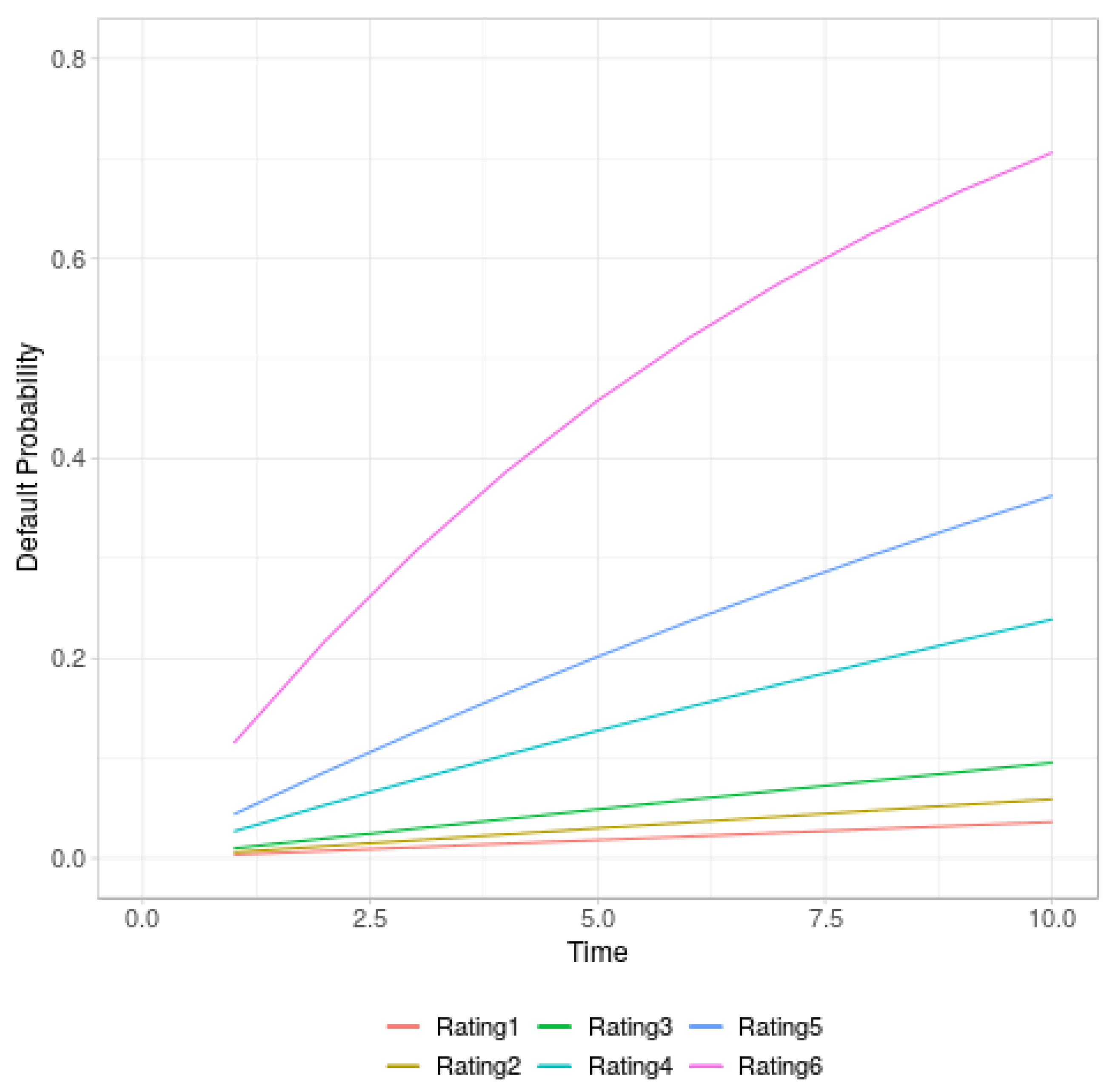
For the evaluation of default risk, we assume that a bank has established a rating system with six grades and uses a Cox proportional hazard model (
10) to estimate term-structures of default probabilities. We assume that the loan’s interest rate is part of one risk factor, all other risk factors are summarized in the coefficient
and
h is a constant as in (
29). The parameters for each rating grade are summarized in
Table 2 while the default probabilities for each rating grade are illustrated in
Figure 1 using the interest rate of the example, 4%.
It remains to define economic capital and the operating costs of the bank. We assume an annual operating cost margin . Economic capital is computed following the regulatory rules for corporate clients with an annual turnover above 50 million EUR where we use both the Standardized and the Internal Ratings Based Approach in our examples. In the case of the Standardized Approach, we assume that the company does not have an external rating. Finally, we assume a target RAROC of 10%.
Cost components and RAROC are computed for the collateralized bullet loan (Loan I), the unsecured bullet loan (Loan II), the collateralized installment loan (Loan III), and the unsecured installment loan (Loan IV). The borrower rating is “3”, i.e., we assume a borrower with a one-year default probability of roughly 1%. The results are summarized in
Table 3 when
E is computed as
and in
Table 4 when
E is computed by (
22).
The quantities
and
show the effect of the amortization rate. Both the swap curve and the funding spreads curve are steep. Since an amortization rate reduces the effective maturity of a loan both quantities are lower for amortizing loans. This effect is not seen in
because both basis swap spread curves are flat. The expected loss margin
is considerably higher for the unsecured loan. For the amortizing collateralized loan, the expected loss margin is lowest because this loan becomes less risky when the outstanding balance is reduced due to the amortizations. This effect is not seen in
E in
Table 4 because economic capital is based on a one-year horizon in the Basel II setup. We see that in both tables, only the collateralized loans pass the RAROC target of 10%. The unsecured loans show a RAROC below 10% and should be rejected if a bank strictly sticks to its profitability target.
In the second example, we compute
,
and maximum RAROC for Loan IV. Again we present the results for both regulatory regimes. The outcome for the Standardized Approach is displayed in
Table 5 while the numbers for the Internal Ratings Based Approach are shown in
Table 6.
We see that for the high-risk clients, no hurdle rate
exists. This means that it is not possible for a bank to set an interest rate that makes the loan profitable. Therefore, a loan application of these clients should be rejected. We see that for Rating “3” in both cases, the hurdle rate is above 4%. This is consistent with the results in
Table 3 and
Table 4 where RAROC was below the profitability target of 10% for Loan IV when an interest rate of 4% was used. Consistent with intuition, in both cases
is increasing with borrower default risk while
and
are decreasing.
7. Discussion
In this article, a loan pricing scheme is developed using the performance measure RAROC. Motivated by balance sheet considerations, i.e., the desire to match assets and liabilities, a calculation scheme is proposed which explicitly decomposes a loan’s interest rate into relevant cost components: Funding costs, costs for hedging interest rate risks, expected loss costs, target return on economic capital, and internal bank costs. For fixed-rate loans, a formula for the base swap rate was given in addition. These cost components are essential for internal fund transfer pricing processes between separate functions in a bank.
The proposed pricing scheme is applicable for loans with the deterministic interest rate, i.e., fixed-rate loans and floating-rate loans linked to Ibor rates. We have analyzed the scheme mainly for the case where term-structures of default probabilities are estimated using a Cox proportional hazard model. This was motivated by the analytical tractability of this model. However, the scheme does not depend on this modeling assumption and could work with any term-structure of default probabilities regardless of its determination.
In a theoretical analysis, it was shown in a slightly simplified setup that if a borrower’s default probability increases with a loan’s interest rate then RAROC becomes in the limiting cases of arbitrarily large negative and positive interest rates which means that both the cases of bank and borrower bankruptcy are treated within economic intuition by RAROC. It was further shown that RAROC has a unique maximum and that at most a finite interval of interest rates exists at which a bank should accept a loan application. In cases where interest rates a borrower is willing to accept are outside this interval or when the acceptance range is empty, a bank should reject a loan application.
Numerical examples illustrated the application of this loan pricing framework. The examples suggest that the main results of the article hold in a more general setup than we were able to prove formally. The main challenge of applying this framework in practice is finding a link between a loan’s interest rate and borrower default rates empirically. In real data sets important information for determining this relationship like the total interest a borrower is paying on all his existing loan products or timely income information is often missing in retail data sets which makes the parameters and of our examples very hard to estimate.
The benefits of implementing this approach in practice are threefold. First, the scheme delivers a split of a loan’s interest rate into cost components for internal fund transfer pricing. Second, when interest rate costs are properly included in a credit scorecard, the scheme allows the calculation of the profitability range for a loan. Only rates within this range a bank should offer when originating a loan. Finally, since the scheme delivers a loan valuation, it could, in addition, be valuable in the price determination of loan portfolio transactions when loans are sold to investors.
One shortcoming of the profitability range is that this interest rate interval models only the perspective of the bank. These are the interest rates that ensure that the profitability requirements of the bank are met, but there is no view from the borrower’s perspective included. It would be very helpful if a bank would have, in addition to the profitability range, some information about the likelihood that a borrower will accept a loan offer and how this likelihood changes within the profitability range.
Chun and Lejeune (
2020) use the probability that a borrower accepts a loan offer in their model but merely on a theoretical basis using several distribution functions without giving any suggestion on empirical verification. Complementing the profitability range by including the borrower perspective would further increase the value of the RAROC scheme. We leave this challenging task for future research.


