Article

Hedging with Liquidity Risk under CEV Diffusion

1
Asset Management Department, Daishin Securities, Seoul 06131, Korea
2
Department of Statistics, Purdue University, West Lafayette, IN 47907, USA
*
Author to whom correspondence should be addressed.
These authors contributed equally to this work.
Risks 2020, 8(2), 62; https://doi.org/10.3390/risks8020062
Submission received: 30 April 2020 / Revised: 23 May 2020 / Accepted: 1 June 2020 / Published: 5 June 2020

Abstract

:
We study a discrete time hedging and pricing problem in a market with the liquidity risk. We consider a discrete version of the constant elasticity of variance (CEV) model by applying Leland’s discrete time replication scheme. The pricing equation becomes a nonlinear partial differential equation, and we solve it by a multi scale perturbation method. A numerical example is provided.

Graphical Abstract

1. Introduction

Liquidity risk is the risk caused by the adverse movement of a price which corresponds to a trading size. A large buy order drives the price up and a large sale order drives it down. Therefore, a large trader is always exposed to this hidden possible loss. Although the idea that the evolution of the stock price depends on the trading volume has existed for several decades, it was not widely studied until only about a decade ago. In the past decade, the literature on the liquidity risk has been growing rapidly; for example, Jarrow (1992, 1994, 2001); Back (1993); Frey (1998, 2000); Frey and Stremme (1997); Cvitanic and Ma (1996); Subramanian and Jarrow (2001); Duffie and Ziegler (2001); Bank and Baum (2004); Cetin et al. (2004); Jarrow (1992, 1994) proposed a discrete-time framework where prices depend on the large trader’s activities via a reaction function of his/her instantaneous holdings. He found conditions for the existence of arbitrage opportunities for a large trader. Cvitanic and Ma (1996) studied a diffusion model for the price dynamics where the drift and volatility coefficients depend on the large investor’s trading strategy. Frey and Stremme (1997) developed a continuous-time analogue to Jarrow’s discrete-time framework. They derived an explicit expression for the transformation of market volatility with a large trader.
Although the cost caused by the liquidity risk have been studied widely both theoretically and empirically, most models in mathematical finance did not include it. Cetin et al. (2004, 2006) introduced a rigorous mathematical model of the liquidity cost and showed modified fundamental theorems of the asset pricing. Bank and Baum (2004) introduced a general continuous-time model for an illiquid financial market with a single large trader. They proved the absence of arbitrage for a large trader, characterized the set of approximately attainable claims and showed how to compute superreplication prices. Studies related to this topic extend to Cetin et al. (2010); Rogers and Singh (2010).
Ku et al. (2012) studied a discrete time hedging strategy with liquidity risk under the Black-Scholes model Black and Scholes (1973). They used the Leland discretization scheme to find the optimal discrete time hedging strategy under the Black-Scholes model. As an extension of it, we study in this paper a more general underlying model which is called the constant elasticity of variance (CEV) model. The CEV model generalizes the Black-Scholes model so that it can capture volatility smile effect. The model is widely used by practitioners in the financial industry, especially to model equities and commodities. The CEV model, introduced by Cox (1975); Cox and Ross (1976) is the following,
d S t = μ S t d t + σ S t θ ˜ 2 d W t , 0 t T , .
Here, θ ˜ (elasticity), μ (mean return rate) and σ (volatility) are given constants. Note that the particular case θ ˜ = 2 corresponds to the well-known Black-Scholes model Black and Scholes (1973).
On the other hand, many underlying assets are still approximately close to a log-normal distribution. This suggests that the elasticity constant θ ˜ is not exactly 2, but is close to 2. In this sence, we set θ ˜ : = 2 θ to apply the asymptotic analysais where 0 θ < 1 .
In Cetin et al. (2004, 2006), the stock price S ( t , x ) depends on the time t and trading volume x. They assume the multiplicative model S ( t , x ) = f ( x ) S ( t , 0 ) , where f is smooth and increasing function with f ( 0 ) = 1 . S ( t , 0 ) becomes a marginal stock price. Empirical studies suggest that the liquidity cost is relatively small compared to the stock price, as in Cetin et al. (2006). In other words, f ( 0 ) is a small positive number. We refer to Cetin et al. (2006) for details.
These two observations motivate us to use the perturbation theory Hinch (2003) for partial differential equations (PDEs) in the liquidity risk problem. The perturbation method is a mathematical method for obtaining an approximate solution to a given problem which cannot be solved exactly, by starting from the exact solution of a related problem. Perturbation theory is used when the problem is formulated by a small term to a mathematical description of the exactly solvable problem. For example, see Park and Kim (2011). Perturbation theory is a useful tool to deal with liquidity risk under the CEV diffusion model based on some small parameters. It gives us a practical advantage in pricing of financial derivatives with the liquidity risk.
The CEV diffusion model is the easiest model to explain the volatility smile phenomenon. It has the disadvantage that the implied volatility estimated by the deep OTM(Out of The Money) option does not match the actual data, but it is easy to apply and the accuracy is guaranteed near the ATM(At The Money). Therefore, when reflecting the skewed phenomenon and hedge the options near ATM, it has a practical advantage compared to the stochastic volatility model. However, it is inadequate to deal with the hedge of a complex structured derivatives, which is inadequate compared to the stochastic volatility model, and subsequent studies need to address the liquidity model under the stochastic volatility model.
We study the liquidity risk under the CEV diffusion model. We apply the Leland approximation scheme (Leland 1985) to obtain a nonlinear partial differential equation for the option pricing. We find an approximation solution of this problem using the perturbation method.
The rest of this paper is organized as follows. Section 2 introduces the Cetin et al. model and the CEV diffusion. Section 3 gives us a nonlinear partial differential equation for the option pricing with the liquidity cost. Section 4 discusses an analytic solution for the PDE given in Section 3.

2. Model

2.1. Background on Liquidity Risk

First, we recall concepts introduced by Cetin et al. (2004). We consider a probability space ( Ω , F , ( F t ) 0 t T , P ) where P is an empirical probability measure, and filtration, ( F t ) 0 t T , satisfies the usual conditions. We consider a market which consists of a risky asset (stock) and a money market account. There is no dividend and the spot rate of interest is zero without loss of generality. S ( t , x , ω ) is the stock price per share at time t that the trader pays/receives for an order of size x R . Here, positive x > 0 means a buy-initiated order and negative x < 0 means a sale-initiated one. A zeroth order x = 0 means a marginal trade. We refer to Cetin et al. (2004) for detailed discussions.
A portfolio ( ( X t , Y t : t [ 0 , T ] ) , τ ) is a triplet, where X t is the trader’s aggregate stock holding at t, Y t is the money market account position, and τ represents the liquidation time of the stock position. Also, we assume that X t and Y t are predictable and optional processes, respectively, and X 0 = Y 0 = 0 .
A self-financing strategy is a trading strategy ( ( X t , Y t : t [ 0 , T ] ) , τ ) where
Y t = Y 0 + X 0 S ( 0 , X 0 ) + 0 t X u d S ( u , 0 ) X t S ( t , 0 ) 0 u t Δ X u [ S ( u , Δ X u ) S ( u , 0 ) ] 0 t S ( t , 0 ) x d [ X , X ] u c .
The second line of (2) represents the loss due to the liquidity cost. Therefore, it is natural to define the liquidity cost by
L t = 0 u t Δ X u [ S ( u , Δ X u ) S ( u , 0 ) ] + 0 t S ( t , 0 ) x d [ X , X ] u c .
Note that L t is always non-negative.

2.2. Model: CEV Diffusion

Let S ( t , 0 ) = S t be the marginal price of the supply curve. We assume that S t follows the next stochastic differential equation (SDE)
d S t = μ S t d t + σ S t 2 θ 2 d W t , 0 < t T , S 0 = s .
Here, θ , μ and σ are given positive constants. A particular case θ = 0 corresponds to the Black-Scholes model.
Cox (1975); Cox and Ross (1976) introduced the constant elasticity of variance (CEV) model as an extension of the Black-Scholes model Black and Scholes (1973). CEV model explains a non-flat geometry of the implied volatility, while the Black-Scholes model does not. In this sense, the CEV model is a good generalization of the Black-Scholes model.
Let us consider the partition of time 0 = t 0 < t 1 < , t n = T with Δ t i : = t i t i 1 for i = 1 , , n . We set the partition Δ t i = Δ t j : = Δ t for all i , j = 1 , , n for simplicity. Then, we consider the following discrete version of (4)
Δ S t i + 1 = μ S t i Δ t + σ S t i θ 2 Δ W t = μ S t i Δ t + σ S t i θ 2 Z Δ t ,
where Z is a standard normal random variable. We assume that a multiplicative supply curve
S ( t , x ) = f ( x ) S t ,
where f is a smooth and increasing function with f ( 0 ) = 1 . f ( x ) represents a change of stock price caused by the liquidity. Since we observe that rate of change at x = 0 is positive and relatively small, f ( 0 ) is positive and close to 0. Therefore, we assume that 0 < f ( 0 ) = ϵ < 1 for a constant ϵ . (We refer to Cetin et al. (2006) for details)
In a discrete time trading, the liquidity cost becomes
L t = i = 1 n Δ X i [ S ( t i , Δ X i ) S ( t i , 0 ) ] ,
where Δ X i = X t i X t i 1 .
Let C t denote the value of the contingent claim. Then, the hedging error becomes
i = 0 n 1 X i ( S t i + 1 S t i ) C T + C 0 L T .

3. The Pricing Equation

We consider a European put option P ( T , s ) = ( K s ) + with the expiration date T with the strike price K, and let P ( t , S t ) be the price of it at time t. (We can similarly deal with call options and other European options, however, we only deal with a put option here.) We consider the delta hedging X t defined by
X t i = P s | s = S t i
for a price function P. Although the market is still complete, since we deal with a discrete time trading with the liquidity cost, a perfect hedging is not possible. Therefore, we cannot make the hedging error 0. However, we can provide a sufficient pricing equation whose expected hedging error approaches zero as Δ t 0 . We assume that P ( t , S t ) is a class of C 1 , 3 ( [ 0 , T ) × R ) .
The next theorem gives us a hedging strategy which makes the expected hedging error go to 0 as the size of the time step gets smaller. Recall that f ( 0 ) = ϵ .
Theorem 1.
Let P ( t , s ) be the solution of the nonlinear partial differential equation
P t + 1 2 σ 2 s 2 θ 2 P s s ( 1 + 2 ϵ s 2 P s s ) = 0 ,
with the terminal condition P ( T , s ) = ( K s ) + . Then the expected hedging error of the corresponding delta hedging strategy approaches 0 as Δ t 0 .
Proof. 
First, we consider Taylor expansion formulas of P, X.
P ( t + Δ t , S + Δ S ) P ( t , S ) = P t Δ t + P s Δ S + 1 2 2 P s s ( Δ S ) 2 + O ( Δ t 3 / 2 ) ,
X ( t + Δ t , S + Δ S ) X ( t , S ) = 2 P t s Δ t + 2 P s s Δ S + 1 2 3 P s s s ( Δ S ) 2 + O ( Δ t 3 / 2 ) .
From (7) and S ( t , x ) = f ( x ) S ( t , 0 ) , we have
Δ X ( S ( t , Δ x ) S ( t , 0 ) ) = Δ X ( f ( Δ X ) 1 ) S t .
On the other hands, by the Taylor expansion formula, we also have
f ( x ) 1 = f ( x ) f ( 0 ) = f ( 0 ) x + 1 2 f ( 0 ) x 2 + O ( x 3 ) .
Moreover, from (5),
( Δ S ) 2 = σ 2 S t 2 θ Z 2 Δ t + O ( Δ t 3 / 2 )
( Δ S ) k = O ( Δ t 3 / 2 ) , k = 3 , 4 , .
Therefore, (12) becomes
Δ X ( S ( t , Δ x ) S ( t , 0 ) ) = Δ X f ( 0 ) Δ X + 1 2 f ( 0 ) ( Δ X ) 2 S t + O ( Δ t 3 / 2 ) = f ( 0 ) σ 2 Z 2 ( S t ) 3 θ 2 P s s Δ t + O ( Δ t 3 / 2 ) = ϵ σ 2 Z 2 ( S t ) 3 θ 2 P s s Δ t + O ( Δ t 3 / 2 ) .
Now, the hedging error is
Δ H = X Δ S Δ P Δ X ( S ( t , Δ X ) S ( t , 0 ) ) = P t Δ t 1 2 σ 2 Z 2 ( S ) 2 θ 2 P s s ( 1 + 2 ϵ S 2 P s s ) Δ t + O ( Δ t 3 / 2 ) .
Since Z is a standard normal, we have
E [ Δ H ] = E [ P t Δ t 1 2 σ 2 Z 2 ( S ) 2 θ 2 P s s ( 1 + 2 ϵ S 2 P s s ) Δ t + O ( Δ t 3 / 2 ) ] = E [ P t + 1 2 σ 2 Z 2 ( S ) 2 θ 2 P s s ( 1 + 2 ϵ S 2 P s s ) ] Δ t + O ( Δ t 3 / 2 ) .
Therefore, E [ Δ H ] = O ( Δ t 1 / 2 ) if P satisfies
P t + 1 2 σ 2 ( S ) 2 θ 2 P s s ( 1 + 2 ϵ S 2 P s s ) = 0 .
Finally, the terminal condition follows from the definition of the put option. □
We notice that the the effect of the liquidity cost appear through the first derivative f ( 0 ) = ϵ . We now study the convergence of the discrete hedging strategy to the payoff of the option. Let Δ H i be the hedging error over [ t i 1 , t i ] , i = 1 , , n .
Theorem 2.
Consider the discrete hedging strategy ( X = P s , Y = P X ) where P ( t , s ) is a solution of the Equation (9). Its value at the terminal time T converges almost surely to the payoff of the option as Δ t 0 .
Proof. 
Since P ( t , s ) is smooth, we can check that
E [ ( Δ H i ) 2 ] M ( Δ t ) 2
where M is a constant which does not depend on t [ 0 , T ] . Therefore, we have
E [ Δ H i Δ t | F t i 1 ] = 0 , for all i .
Moreover, we have
lim n i = 1 n 1 i 2 E [ ( Δ H i Δ t ) 2 ] M lim n i = 1 n 1 i 2 < .
Therefore, by the Law of Large Numbers for Martingales (refer to Feller 1970), we obtain
lim n 1 T i = 1 n Δ H i = lim n 1 n i = 1 n Δ H i Δ t = 0 a . s . .
This implies that the total error Δ H i 0 as Δ t 0 a.s.. □
The above theorem tells us that the delta hedging strategy in Equation (9) asymptotically replicates the contingent claim as the time interval gets smaller. So, the next step is to calculate P ( t , s ) so that we can calculate the corresponding hedging strategy. We study this in the following section.

4. Asymptotic Expansion of the Solution

In this section, we discuss an analytic solution of the Equation (9). Since P ( t , s ) satisfies the nonlinear partial differential equation (NPDE) (9), it is hard to find a closed form solution. However, as we already discussed before for the expansion of f, we can apply the asymptotic expansion to (9). We first assume that there exists a series
P 0 , 0 ( t , s ) + ϵ P 0 , 1 ( t , s ) + θ P 1 , 0 ( t , s ) + ϵ θ P 1 , 1 ( t , s ) +
such that P ( t , s ) = l , m = 0 θ l ϵ m P l , m ( t , s ) . Now, we reformulate the NPDE (Nonlinear Partial Differential Equations) (9),
P t + 1 2 σ 2 s 2 θ 2 P s s ( 1 + 2 ϵ s 2 P s s ) = P t + 1 2 σ 2 e θ ln s s 2 2 P s s ( 1 + 2 ϵ s 2 P s s ) = P t + 1 2 σ 2 k = 0 ( ln s ) k k ! θ k s 2 2 P s s ( 1 + 2 ϵ s 2 P s s ) = P t + k = 0 θ k 1 2 σ 2 ( ln s ) k k ! s 2 2 P s s + k = 0 ϵ θ k σ 2 ( ln s ) k k ! s 3 ( 2 P s s ) 2 = 0 .
Note that the first term is an ϵ 0 θ 0 order term, the second is an ϵ 0 θ k order one, and the third term is an ϵ 1 θ k term. Inserting these series form into (24), we obtain following equations for each coefficient P l , m ( t , s ) for l , m = 0 , 1 , ,
P 0 , 0 t + 1 2 σ 2 s 2 2 P 0 , 0 s s = 0
P 0 , 1 t + 1 2 σ 2 s 2 2 P 0 , 1 s s = σ 2 s 3 ( 2 P 0 , 0 s s ) 2
P 1 , 0 t + 1 2 σ 2 s 2 2 P 1 , 0 s s = 1 2 σ 2 s 2 2 P 0 , 0 s s ,
where terminal conditions are given by P 0 , 0 ( T , s ) = ( K s ) + and P 0 , 1 ( T , s ) = P 1 , 0 ( T , s ) = = 0 . In general, we obtain the partial differential equation for P l , m ( t , s ) ,
P l , m t + 1 2 σ 2 s 2 2 P l , m s s = G l , m ( t , s ) G l , m ( t , s ) : = k = 1 l 1 2 σ 2 ( ln s ) k k ! s 2 2 P l k , m s s k = 0 l i 1 + i 2 = l k , j 1 + j 2 = m 1 σ 2 ( ln s ) k k ! s 3 2 P i 1 , j 1 s s 2 P i 2 , j 2 s s
where P 1 , · = P · , 1 : = 0 .

4.1. A Solution of Each Coefficient

To find P l , m for l , m = 0 , 1 , 2 , , we need a lemma about the Feynman-Kac formula for our nonhomogeneous PDE. First, we define a geometric Brownian motion S ˜ t by
d S ˜ t = σ S ˜ t d W t , 0 t T ,
and a differential operator
L 0 : = t + 1 2 σ 2 s 2 2 s s .
Then, we have the following.
Lemma 1.
If the solution u ( t , s ) of the PDE problem
L 0 u ( t , s ) = f ( t , s ) , 0 t < T ,
u ( T , s ) = h ( s )
satisfies the condition u ( t , s ) C 1 , 2 ( [ 0 , T ] × R ) and f , h L , then u ( t , s ) is given by
u ( t , s ) = E s [ h ( S ˜ T ) t T f ( s , S ˜ s ) d s ] . E s [ · ] : = E P [ · | S ˜ t = s ] .
Proof. 
This is the well-known Feynman-Kac formula for the Black-Scholes model. It provides a stochastic representation of the solution of PDEs. We refer to the chapter 8 of Oksendal (2003) for details. □
The next theorem give us P 0 , 0 , which is the first term of the expansion.
Theorem 3.
The leading order solution P 0 , 0 ( t , s ) is given by
P 0 , 0 ( t , s ) = s N ( d 1 ) + K N ( d 2 ) , d 1 , 2 : = ln s K ± 1 2 σ 2 ( T t ) σ T t , N ( x ) : = 1 2 π x e z 2 2 d z .
Proof. 
By Lemma 1, we have
P 0 , 0 ( t , s ) = E [ ( K S ˜ T ) + | S ˜ t = s ] .
This is the well-known Black-Scholes put option price. We refer to Shreve (2000) for details. □
Next, we find a solution of remaining terms P l , m for general l and m.
Theorem 4.
For l , m 0 , the solution P l , m ( t , s ) is recursively given by
P l , m ( t , s ) = t T G l , m ( τ , s e 1 2 σ 2 ( τ t ) + σ x ) 2 π ( τ t ) e x 2 2 ( τ t ) d τ d x .
Proof. 
First, we consider the case l = 0 , m = 1 . In this case, G l , m ( t , s ) = σ 2 s 3 ( 2 P 0 , 0 s s ) 2 . Since P 0 , 0 ( t , s ) is smooth on only t [ 0 , T ) and continuous at t = T , we have to deal with it carefully. First, note that there exist a smooth function f n ( t , s ) on [ 0 , T ] × R such that lim n f n = P 0 , 0 ( t , s ) . Now we consider the PDE
F n t + 1 2 σ 2 s 2 2 F n s s = σ 2 s 3 ( 2 f n s s ) 2 ,
where F n ( T , s ) = 0 . By Lemma 1, we have
F n ( t , s ) = E s [ t T σ 2 ( S ˜ τ ) 3 ( 2 f n s s ) ( τ , S ˜ τ ) ) 2 d τ ] .
It is well-known that the solution of PDE u t + 1 2 σ 2 s 2 2 u s s = 0 and u ( T , s ) = 0 is u = 0 (the uniqueness of a solution). Therefore, F n P 0 , 0 as n . By the dominated convergence theorem, we have
P 0 , 1 = lim n E s [ t T σ 2 ( S ˜ τ ) 3 ( 2 f n s s ( τ , S ˜ τ ) ) 2 d τ ] = E s [ t T σ 2 ( S ˜ τ ) 3 ( 2 P 0 , 0 s s ( τ , S ˜ τ ) ) 2 d τ ] .
On the other hand, S ˜ τ = s e 1 2 σ 2 ( τ t ) + σ W τ t leads to
P 0 , 1 = E s [ t T σ 2 ( S ˜ τ ) 3 ( 2 P 0 , 0 s s ( τ , S ˜ τ ) ) 2 d τ ] = E s [ t T σ 2 ( S ˜ τ ) 3 e 3 2 σ 2 ( τ t ) + 3 σ W τ t ( 2 P 0 , 0 s s ( τ , s e 1 2 σ 2 ( τ t ) + σ W τ t ) ) 2 d τ ] = t T σ 2 s 3 e 3 2 σ 2 ( τ t ) + 3 σ x ( 2 P 0 , 0 s s ( τ , s e 1 2 σ 2 ( τ t ) + σ x ) ) 2 1 2 π ( τ t ) e x 2 2 ( τ t ) d τ d x .
Moreover, P 0 , 1 ( t , s ) is twice continuously differentiable with respect to s. On the other hand, we can obtain the similar result for P 1 , 0 using the same argument. Now, we use the induction argument. Suppose that G l , m satisfies the assumption of Lemma 1. Then we have
P l , m = E s [ t T G l , m ( τ , S ˜ τ ) d τ ] = E s [ t T G l , m ( τ , s e 1 2 σ 2 ( τ t ) + σ W τ t ) d τ ] = t T G l , m ( τ , s e 1 2 σ 2 ( τ t ) + σ x ) 2 π ( τ t ) e x 2 2 ( τ t ) d τ d x .
Using the above theorem, we can calculate P ( t , s ) and the corresponding hedging strategy X t . While it is hard to calculate these quantities analytically, we can calculate these relatively easily numerically. 
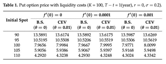
Table 1 shows the European put option price with the liquidity cost computed by our approximation formula. We present an approximate option price, P ( t , s ) P 0 , 0 ( t , s ) + ϵ P 0 , 1 ( t , s ) + θ P 1 , 0 ( t , s ) . Option prices are obtained by solving the formula given in Theorem 4. Parameters that we use here are K = 100 , σ = 0.2 , r = 0 and T t = 1 year. Table 1 presents numerical results for several cases. We use the formula (31) and numerical integration for the first order ( l = 1 or m = 1 ) calculation. The first example, f ( 0 ) = 0 is the case without the liquidity cost. In this case, we can buy and sell the underlying asset at the spot price. However, in reality, the liquidity provider quotes different prices for buying and selling, and the liquidity cost does exist. So we can only buy or sell the underlying asset after adding the bid and ask spread. The second and the third cases are when the regular bid and ask spread rates are 0.000001 and 0.00001 percent of spot, respectively. The second case, f ( 0 ) = 0.0001 , considers 0.000001 percent spread of the spot price. For example, if the spot price is 10000 dollars, then the spread is one cent. This means that liquidity risk causes an additional hedge cost for the dynamic hedging that is, we need more asset and funding money. This comparison result is reasonable in the sense that a higher liquidity cost produces a bigger option premium for the same spot price. Since the liquidity cost makes the hedging cost higher, an option price should be higher for a bigger liquidity cost. In addition, the CEV parameter provides a non-flat volatility risk. Therefore, the CEV option price should be higher than the Black-Scholes price. We observe this from the fact that the second column is larger than the first column.
Remark 1.
For a practical application, we can apply our method as follows. From real market data, we observe two small parameters ϵ and θ. Then, we can apply the perturbation method for this problem. By applying the perturbation method, we can derive an approximation solution of option price with liquidity costs.

4.2. Convergence of the Series

In this subsection, we study the convergence of
l , m = 0 θ l ϵ m P l , m ( t , s ) = P ( t , s ) .
Previously, we assumed that the existence of the series. However, to guarantee the existence of the series, we need to prove it. In this case, the existence of the series is equivalent to convergence of the series. Therefore, we show the convergence. Let P l , m ( t , s ) : = sup t , s | P l , m ( t , s ) | , then we have the following.
Theorem 5.
For all l , m = 0 , 1 , , we have
P l , m ( t , z ) < .
Proof. 
First, we show P 0 , 1 ( t , s ) < . Note that | P 0 , 0 ( t , s ) | K where K is the exercise price. Moreover, s 2 P 0 , 0 ( t , s ) s s = e ( d 1 ) 2 2 σ 2 π ( T t ) and s 2 2 P 0 , 0 ( t , s ) s s = e ln s + ( d 1 ) 2 2 σ 2 π ( T t ) are o ( e s 2 ) as s and bounded by 1 2 σ T , since ln s + ( d 1 ) 2 2 < 0 for all s > 0 . By the probabilistic representation of P 0 , 1 , we have
P 0 , 1 ( t , s ) = E s [ t T σ 2 ( S ˜ τ ) 3 ( 2 P 0 , 0 s s ( τ , S ˜ τ ) ) 2 d τ ] E s [ t T σ 2 1 2 σ T 1 2 σ T d τ ] 1 4 .
On the other hand, the integration formula of P 0 , 1 ( t , s ) implies that P 0 , 1 ( t , s ) and s k 2 P 0 , 1 ( t , s ) s s , k = 1 , 2 are also o ( e s 2 ) as s . Therefore, all of them are bounded and infinitely differentiable. By the same argument, we have the same result for P 1 , 0 ( t , s ) . Now, we apply the induction. Suppose that P i , j ( t , s ) for i = 0 , 1 , , l 1 , j = 0 , 1 , , m and P i , j ( t , s ) and s 2 P i , j ( t , s ) s s are smooth and bounded. Then, we have
| P l , m ( t , s ) | = | E s [ t T G l , m ( τ , S ˜ τ ) d τ ] | E s [ t T | k = 1 l 1 2 σ 2 ( ln S ˜ τ ) k k ! S ˜ τ ( S ˜ τ 2 P l k , m s s ( τ , S ˜ τ ) ) | d τ ] + E s [ t T | k = 0 l i 1 + i 2 = l k , j 1 + j 2 = m 1 σ 2 ( ln S ˜ τ ) k k ! S ˜ τ 3 2 P i 1 , j 1 s s 2 P i 2 , j 2 s s ( τ , S ˜ τ ) | d τ ] c 0 E s [ t T | k = 0 l 3 2 σ 2 ( ln S ˜ τ ) k k ! S ˜ τ | d τ ] ,
where c 0 is a positive constant determined by s 2 P i 1 , j 1 s s . Then,
E s [ t T | k = 0 l 3 2 σ 2 ( ln S ˜ τ ) k k ! S ˜ τ | d τ ] = E s [ t T | k = 0 l 3 2 σ 2 ( ln S ˜ τ ) k k ! S ˜ τ | d τ ] t T E s [ k = 0 l 3 2 σ 2 ( ln S ˜ τ ) k k ! S ˜ τ ] d τ 3 2 σ 2 t T E s [ ( S ˜ τ ) 2 ] d τ .
On the other hand, e μ t S ˜ t is a martingale under P . Let S ˜ T : = max t [ 0 , T ] S ˜ t . Then, by the Doob’s maximal inequality, we have
t T E s [ ( S ˜ τ ) 2 ] d τ t T E s [ ( S ˜ τ ) 2 ] d τ T E P [ ( S ˜ T ) 2 ] 4 T E P [ ( S ˜ T ) 2 ] < .
This implies that P l , m < . Moreover, the integration formula of P l , m ( t , s ) implies that P l , m ( t , s ) and s 2 P l , m ( t , s ) s s are also o ( e s 2 ) as s . Therefore, by the induction argument, we have P l , m < for all l , m = 0 , 1 , . □
By the above theorem, the series satisfies
l , m = 0 θ l ϵ m P l , m ( t , s ) l , m = 0 θ l ϵ m P l , m ( t , s ) <
for given 0 < θ , ϵ < < 1 . We now define Φ ( t , s ) : = l , m = 0 θ l ϵ m P l , m ( t , s ) . Clearly, Φ ( T , s ) = ( K s ) + and Φ ( t , s ) satisfies NPDE (24) by (28). Therefore, we can conclude that
l , m = 0 θ l ϵ m P l , m ( t , s ) = P ( t , s )
and
| P ( t , s ) l , m = 0 l = i , m = j θ l ϵ m P l , m ( t , s ) | = o ( θ i ϵ j ) .

5. Conclusions

We studied a delta hedging method with the liquidity risk under the CEV diffusion model. We used the approximation method to find the price and the hedging strategy. Our method is simple but still quite accurate. A simulation study shows that high liquidity cost drove the option price higher, which is intuitively expected.

Author Contributions

Conceptualization, K.L.; methodology, S.-H.P.; validation, S.-H.P.; formal analysis, S.-H.P. and K.L.; writing–original draft preparation, S.-H.P.; writing–review and editing, K.L. All authors have read and agreed to the published version of the manuscript.

Funding

This research received no external funding.

Conflicts of Interest

The authors declare no conflict of interest. The funders had no role in the design of the study; in the collection, analyses, or interpretation of data; in the writing of the manuscript, or in the decision to publish the results.

References

  1. Back, Kerry. 1993. Asymmetric Information and Options. The Review of Financial Studies 6: 435–72. [Google Scholar] [CrossRef]
  2. Bank, Peter, and Dietmar Baum. 2004. Hedging and Portfolio Optimization in Financial Markets with a Large Trader. Mathematical Finance 14: 1–18. [Google Scholar] [CrossRef]
  3. Black, Fischer, and Myron Scholes. 1973. The pricing of options and corporate liabilities. The Journal of Political Economy 81: 637–59. [Google Scholar] [CrossRef] [Green Version]
  4. Cetin, Umut, Robert A. Jarrow, and Philip Protter. 2004. Liquidity Risk and Arbitrage Pricing Theory. Finance and Stochastics 8: 311–41. [Google Scholar] [CrossRef] [Green Version]
  5. Cetin, Umut, Robert Jarrow, Philip Protter, and Mitch Warachka. 2006. Pricing Options in an Extended Black Scholes Economy with Illiquidity: Theory and Empirical Evidence. Review of Financial Studies 19: 493–529. [Google Scholar] [CrossRef] [Green Version]
  6. Cetin, Umut, H. Mete Soner, and Nizar Touzi. 2010. Option hedging for small investors under liquidity cost. Finance and Stochastics 14: 317–41. [Google Scholar] [CrossRef]
  7. Cox, John. 1975. Notes on Option Pricing I: Constant Elasticity of Variance Diffusions. Working Paper. Stanford: Stanford University. [Google Scholar]
  8. Cox, John C., and Stephen A. Ross. 1976. The valuation of options for alternative stochastic processes. Journal of Financial Economics 4: 145–66. [Google Scholar] [CrossRef]
  9. Cvitanić, Jakša, and Jin Ma. 1996. Hedging Options for a Large Investor and Forward-Backward SDE’s. Annals of Applied Probability 6: 370–98. [Google Scholar]
  10. Duffie, Darrell, and Alexandre Ziegler. 2003. Liquidity Risk. Financial Analysts Journal 59: 42–51. [Google Scholar] [CrossRef] [Green Version]
  11. Feller, Willliam. 1970. An Introduction to Probability Theory and Its Applications, 2nd ed. Hoboken: John Wiley & Sons. [Google Scholar]
  12. Frey, Rüdiger. 1998. Perfect Option Hedging for a Large Trader. Finance and Stochastics 2: 115–41. [Google Scholar] [CrossRef]
  13. Frey, Rüdiger. 2000. Risk-Minimization with Incomplete Information in a Model for High-Frequency Data. Mathematical Finance 10: 215–25. [Google Scholar] [CrossRef]
  14. Frey, Rüdiger, and Alexander Stremme. 1997. Market Volatility and Feedback Effects from Dynamic Hedging. Mathematical Finance 7: 351–74. [Google Scholar] [CrossRef]
  15. Hinch, E.J. 1991. Perturbation Methods. Cambridge: Cambridge University Press. [Google Scholar]
  16. Jarrow, Robert A. 1992. Market Manipulation, Bubbles, Corners and Short Squeezes. Journal of Financial and Quantitative Analysis 27: 311–36. [Google Scholar] [CrossRef]
  17. Jarrow, Robert A. 1994. Derivative Security Markets, Market Manipulation and Option Pricing. Journal of Financial and Quantitative Analysis 29: 241–61. [Google Scholar] [CrossRef]
  18. Jarrow, Robert. 2001. Default Parameter Estimation Using Market Prices. Financial Analysts Journal 57: 75–92. [Google Scholar] [CrossRef] [Green Version]
  19. Ku, Hyejin, Kiseop Lee, and Huaiping Zhu. 2012. Discrete time hedging with liquidity risk. Finance Reaserch Letters 9: 135–43. [Google Scholar] [CrossRef]
  20. Leland, Hayne E. 1985. Option Pricing and Replication with Transactions Costs. Journal of Finance 40: 1283–301. [Google Scholar] [CrossRef]
  21. Oksendal, Bernt. 2003. Stochastic Differential Equations, 6th ed. New York: Springer. [Google Scholar]
  22. Park, Sang-Hyeon, and Jeong-Hoon Kim. 2011. Asymptotic option pricing under the CEV Diffusion. Journal of Mathematical Analysis and Applications 375: 490–50. [Google Scholar] [CrossRef] [Green Version]
  23. Rogers, Leonard C. G., and Surbjeet Singh. 2010. The cost of illiquidity and its effects on hedging. Mathematical Finance 20: 597–615. [Google Scholar] [CrossRef] [Green Version]
  24. Shreve, Steven E. 2000. Stochastic Calculus for Finance. New York: Springer, vol. 2. [Google Scholar]
  25. Subramanian, Ajay, and Robert A. Jarrow. 2001. The Liquidity Discount. Mathematical Finance 11: 447–74. [Google Scholar] [CrossRef]
Table 1. Put option price with liquidity costs (K = 100, T t = 1(year), r = 0 , σ = 0.2 ).
Initial Spot f ( 0 ) = 0 f ( 0 ) = 0.0001 f ( 0 ) = 0.001
B.S.CEVB.S.CEVB.S.CEV
( θ = 0 )( θ = 0.01 )( θ = 0 )( θ = 0.01 )( θ = 0 )( θ = 0.01 )
9013.589113.617413.589213.617513.598713.6269
9510.519510.550810.520610.551910.530610.5619
1007.96567.99847.96677.99957.97718.0099
1055.90565.93865.90675.93975.91685.9498
1104.29204.32384.29304.32484.30244.3342

