A Multivariate Model to Quantify and Mitigate Cybersecurity Risk

Abstract

The cost of cybersecurity incidents is large and growing. However, conventional methods for measuring loss and choosing mitigation strategies use simplifying assumptions and are often not supported by cyber attack data. In this paper, we present a multivariate model for different, dependent types of attack and the effect of mitigation strategies on those attacks. Utilising collected cyber attack data and assumptions on mitigation approaches, we look at an example of using the model to optimise the choice of mitigations. We find that the optimal choice of mitigations will depend on the goal—to prevent extreme damages or damage on average. Numerical experiments suggest the dependence aspect is important and can alter final risk estimates by as much as 30%. The methodology can be used to quantify the cost of cyber attacks and support decision making on the choice of optimal mitigation strategies.

1. Introduction

Cyber incidents such as denial of service attacks and data breaches are becoming common and are a major challenge for both businesses and governments around the world. Significant, but limited, resources are devoted to mitigating this risk. There is a need for mathematical modelling techniques to better quantify losses from cyber attack and to find the optimal balance of defences given limited resources. Current methods are either qualitative or too simplistic.

Currently, the majority of risk management decisions are made qualitatively and there is a view, see for instance Munteanu (2017) and Oppliger (2015), that quantitative models are inherently not fit for purpose. It is not advisable to rely exclusively on a quantitative model for decision making purposes. However, we agree with Baskerville (1991) and Geer et al. (2003) that such quantitative models can be an effective framework for quantifying and communicating cyber risk. A quantitative approach has the advantage of forcing transparency about what is considered a threat, the damage caused by those threats, what mitigations are available and the effectiveness and costs of those mitigations.

Quantitative models have of course been developed for cyber risk management. A fundamental approach is that of calculating the Annual Loss Expectancy (ALE), see, e.g., Jacobson et al. (1974). The idea is an intuitive one: the average losses after one year will be the product of the average number of incidents and the average cost a single incident incurs. A good summary of this idea and similar ones is available in Bojanc and Jerman-Blažič (2008). While ALE allows for a back-of-the-envelope calculation, it is deficient in two key areas. Firstly, it gives an expected value rather than a distribution. Knowledge of the distribution allows for calculation of more informative statistics, like Value at Risk (VaR) or Expected Shortfall (see, e.g., Shevchenko 2010). Secondly, it does not allow for different types of attack being made at different rates and with different impacts.

Given a description of possible damages from cybersecurity, a natural question is how to spend limited resources to defend against such incidents. A key paper that looks at this question is Gordon and Loeb (2002). Here, the authors look at optimising the dollar amount spent so as to minimise the overall losses, inclusive of spending on security. The one period setting and the functional form mean the analysis is done in closed form. Modelling of mitigations has since been expanded upon in two directions. The first direction, with a large group of authors, looks at the optimal selection of a portfolio of mitigations; good examples here are Sawik (2013), Viduto et al. (2012) and Zhuo and Solak (2014). In this grouping of papers the focus is not on the underlying risk model but on the role of the mitigations. Often the key tool is constraint programming for choosing correctly from many possible combinations. The second direction, with fewer authors, looks at improving the underlying risk model. Good examples here are Wang (2008) and Lee et al. (2011). The work in Wang (2008) in particular highlights the idea that mitigations may either target lowering the average or the tail of the distribution of losses. The first group of papers does not model the losses as effectively as the second group, which in turn does not model the effect of mitigations as effectively as the first group.

Both groupings of papers suffer from a lack of open data in cyber incidents and a lack of quantitative research on the effect of mitigation strategies. In addition to limited data on cyber incidents (an excellent listing of data sources exists in Eling and Schnell 2016), it is very difficult to get data pertaining to the losses suffered by one organisation. Some data of this form is plotted in Kuypers et al. (2016) and Paté-Cornell et al. (2018). In fact, not only are these the only sources we can find that look at real world data on cyber incidents for one organisation, they are the only sources that look in detail at the effect of mitigations. In Kuypers et al. (2016), the empirical impact of Full Disk Encryption is considered and in Paté-Cornell et al. (2018) the effect of Two Factor Authentication is simulated.

In this paper we suggest the use of a multivariate model for losses from Chavez-Demoulin et al. (2006) and give a model for the effect of mitigations, inspired by that given in Zhuo and Solak (2014). This combination places our work in the gap between the two groupings noted above; using a realistic model for losses as well as a model for the effect of several mitigations. The model for damages comes from the field of operational risk and this is a very natural area to borrow from. Indeed, this observation has been made in Hulthén (2009) and in the book Hubbard and Seiersen (2016). Practitioners in operational risk are of course particularly concerned by the effect of cyber risks (see, e.g., Risk.net 2020). The practical use of this combined model is illustrated by fitting to the data given in Kuypers et al. (2016) and Paté-Cornell et al. (2018) and making assumptions on mitigations from The Australian Signals Directorate (2017). This allows for a distribution of losses to be simulated along with a 5% VaR. Most importantly, it allows for the numerical optimisation of the choice of mitigations given the goal of either minimising VaR or average losses. The combined model serves two purposes.

Firstly, it allows the clear communication of cyber risk to those outside the field. This is useful because the impact of the risk will be obvious and immediate to technicians facing it, but potentially of secondary concern to decision makers who do not face the issue. Such decision makers may be reluctant to spend money on what they view as an unnecessary expense. This mathematical model can be used to quantify the financial impact in dollar terms that would be lost in the absence of proper mitigations, rather than a qualitative and subjective interpretation.

Secondly, such a framework for quantifying cyber risk allows for better decision making on the choice of mitigations. When more realistic assumptions are used, not only can the effect of a particular mitigation strategy be modelled, but the overall effect of different combinations of mitigations be considered. Going further, given many different mitigation strategies, all with different effects and costs, one can find the best combination of these mitigations subject to a fixed budget constraint.

2. Method

In this section we briefly motivate a univariate model for losses. We then outline a multivariate model for losses as in Chavez-Demoulin et al. (2006), giving a result on the mean and variance of losses under the model. We finish by introducing a model for the effect of using different mitigations.

2.1. A Univariate Model for Losses

One can model the losses up to time t as

$$\begin{array}{c}\hfill L(t)=\sum _{i=1}^{N(t)}{X}_i\end{array}$$

where $X_i$ are independent and identically distributed random variables representing the severity of damage from each attack and $N(t)$ is an independent Poisson process with intensity $\lambda$ giving the frequency of attacks. That is, losses can be modelled by a Compound Poisson Process. A description of this process and its properties can be found in, e.g., Ross (2010). One can think of this as the more general setting of ALE, because

$$\begin{array}{c}\hfill \mathbb{E}\left[L(t)\right]=\mathbb{E}\left[N(t)\right]\mathbb{E}\left[X_1\right]\end{array}$$

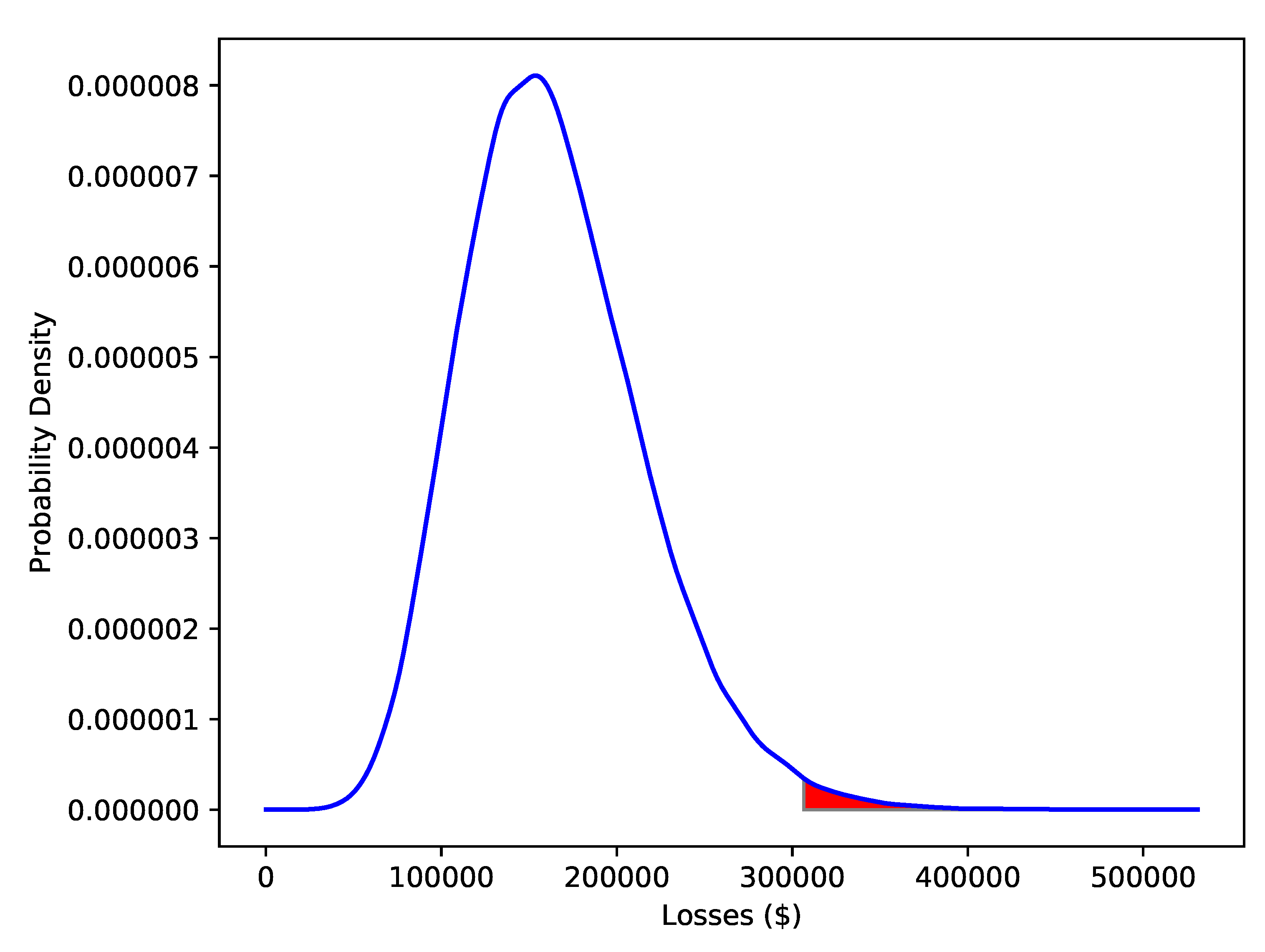
which we can recall is how ALE is defined. The advantage of using such a model over ALE is that we can easily change the specifics of how $L(t)$ is constructed and still get such expressions. Further, there is no reason we have to look at averages. To this end, in the results section in addition to considering expected values, we will calculate various VaR values. Note that this is just another name for a quantile. We use the methodology outlined in Shevchenko (2010) in simulation.

Using a compound Poisson process gives a natural way to model the effect of mitigations on the frequency of attack. If spending z means that attacks succeed with some probability $q(z)$ (instead of always succeeding), the total losses up to time t is still a compound Poisson process, but with intensity $\lambda q(z)$.

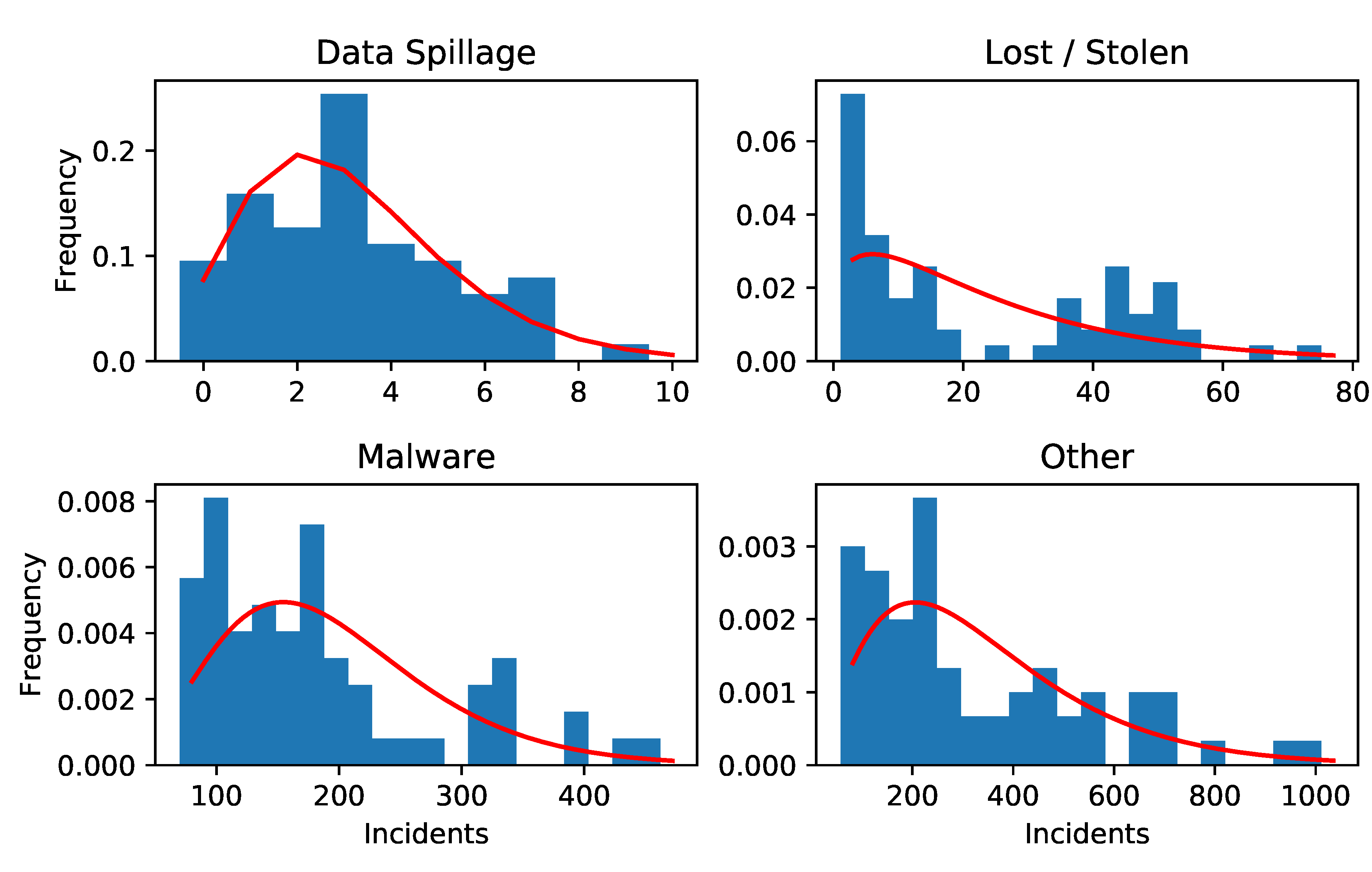
In choosing the parameters of a compound Poisson process, one would first want to find $\lambda$. But the Poisson random variable has the property that its mean is equal to its variance and the data we have is overdispersed. Instead, we will use a counting process that has a Negative Binomial distribution at time t. The Negative Binomial distribution is often used for fitting to count data, and is well known in operational risk. The application of the negative binomial distribution to real world data is done in a cybersecurity context in Leslie et al. (2018).

While it is straightforward to relate a Poisson distribution to the Poisson process, it is not immediately obvious what process has a Negative Binomial distribution. Such a process can be constructed several ways. For instance, one can relate it to a pure birth process, see Toscas and Faddy (2003) for details. A good overview of this distribution is given in Gurland (1959); the following result is read from there with the addition of a thinning probability.

Proposition 1

(Poisson Process with Gamma Intensity is Negative Binomial). Suppose Λ is a Gamma random variable with parameters $\alpha >0$ and $\beta >0$ and q is a probability. If $N(t)$ is a (thinned) Poisson Process with intensity $\Lambda q$, then its distribution at time t is Negative Binomial with parameters $p=qt/(\beta +qt)$ and $r=\alpha$.

Recall that the probability density function of the Gamma distribution is given by

$$\begin{array}{c}\hfill f(x)=\frac{{\beta }^{\alpha }}{\Gamma (\alpha )}{x}^{\alpha -1}{e}^{-\beta x},x>0\end{array}$$

and the probability mass function of the Negative Binomial is given by

$$\begin{array}{c}\hfill Pr(N=n)=\left(\genfrac{}{}{0pt}{}{n+r-1}{n}\right)p^n{(1-p)}^r,n=0,1,2,\dots \end{array}$$

Suppose that we have some count data telling us the number of successful incidents over some time periods $[0,\delta t]$ and the probability q that a given incident is successful. If we find estimates for the parameters as $\widehat{p}$ and $\widehat{r}$, we can find $\alpha$ and $\beta$ as

$$\begin{array}{c}\hfill \begin{array}{cc}\hfill \widehat{\alpha }& =\widehat{r}\hfill \\ \hfill \widehat{\beta }& =\frac{q·(1-\widehat{p})·\delta t}{\widehat{p}}\hfill \end{array}\end{array}$$

(1)

In the sequel, we will change the parameters of the probability of successful attack q by varying the amount spent on different mitigations. The idea we use here is as follows. We find p and r from the data and assume some baseline q. This implies some baseline $\alpha$ and $\beta$ for that assumed q. When we change the spending and hence q, the new p and r that apply are given in terms of those baseline $\alpha$ and $\beta$ by Proposition 1.

To this point we have only described how to model the frequency of attacks. In order to have a complete univariate model for losses we need a model for the severities. Good choices here would include the Lognormal (see for instance Hubbard and Seiersen 2016), Weibull or Power distributions. Due to lack of data, we will use a very simple model for severities described in the Results section.

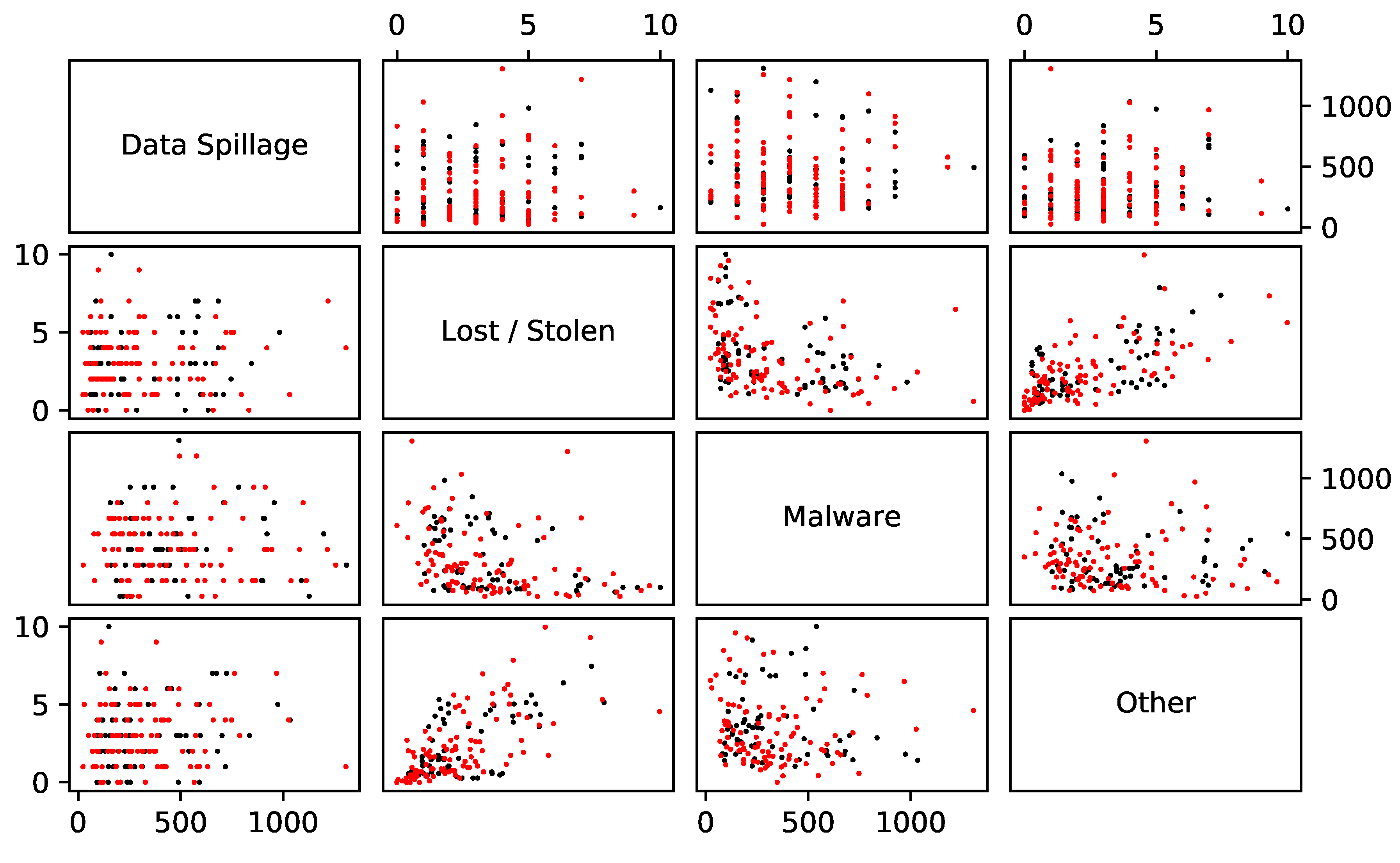
2.2. A Multivariate Model for Losses

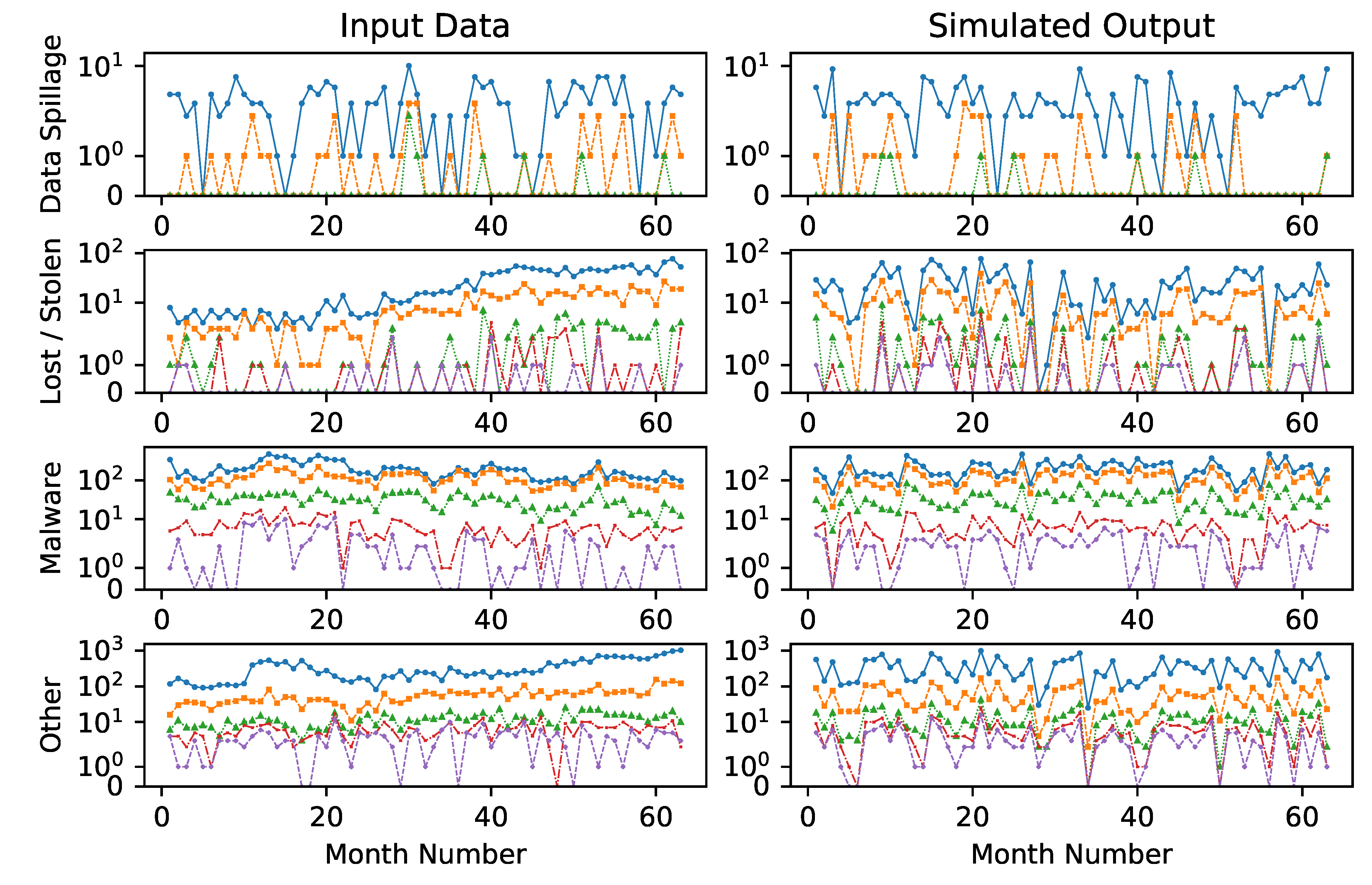
We require a model that is able to handle different, but dependent, categories of damages. There are two components of that requirement. Firstly, we need to handle more than one damage type. For instance, it might be that an organisation faces two types of incidents: an incident of malware or a data spillage event. One would imagine that the first would happen frequently, but have a small impact and that the second would happen rarely but have a large impact. It makes sense to model these incidents separately. The second component of the requirement is an ability to handle dependence between the incidents. For example, it could be that a malware incident sometimes causes a data spillage event.

We suppose there are $j=1,\dots ,J$ categories of damage. It is trivial to make a multivariate model. This can be done by fitting an independent model to each category and summing them. That is, for $j=1,\dots ,J$ we have

$$\begin{array}{c}\hfill L_j(t)=\sum _{i=1}^{N_j(t)}{X}_i^j\end{array}$$

(2)

where the j subscripts relate to the $j^{th}$ type of damage. Our object of interest is then

$$\begin{array}{c}\hfill L(t)=\sum _{j=1}^J{L}_j(t)\end{array}$$

(3)

If the marginal models are all compound Poisson processes, their sum will also be a compound Poisson process. This is very useful because numerical methods can be used to great effect; see Shevchenko (2010), particularly the Fast Fourier Transform based method. Unfortunately simply adding the $L_j(t)$ will not introduce dependence between incident types in our model.

A simple way to include dependence is suggested in Chavez-Demoulin et al. (2006), who look at multivariate operational risk models. Among the ideas presented there is to use a copula function on the marginal frequencies. That is, we have exactly the model in Equations (2) and (3), but we have a multivariate distribution for $(N_1(t),\dots ,N_J(t))$. Ultimately, we will use Monte Carlo simulation to look at the output of such a multivariate model. Because of this, we will restrict our attention to the simulation of a Gaussian copula, rather than looking at the deeper theory of copula functions. For further details on copula functions we note the excellent treatise of Nelsen (1999) and a very practical introduction in Genest and Favre (2007).

A multivariate distribution encodes not only the marginal distributions but their dependence. A copula function is one way of encoding that dependence only. Sklar’s Theorem gives us that combining a copula function with marginal distributions is one way of building a multivariate distribution. Conversely, it also gives us that a given multivariate distribution characterises a copula function. In this vein, a Gaussian copula is the dependence that comes from a multivariate Gaussian distribution; in essence this is equivalent to using linear correlation. Simulating a Negative Binomial random variable under this copula is quite simple.

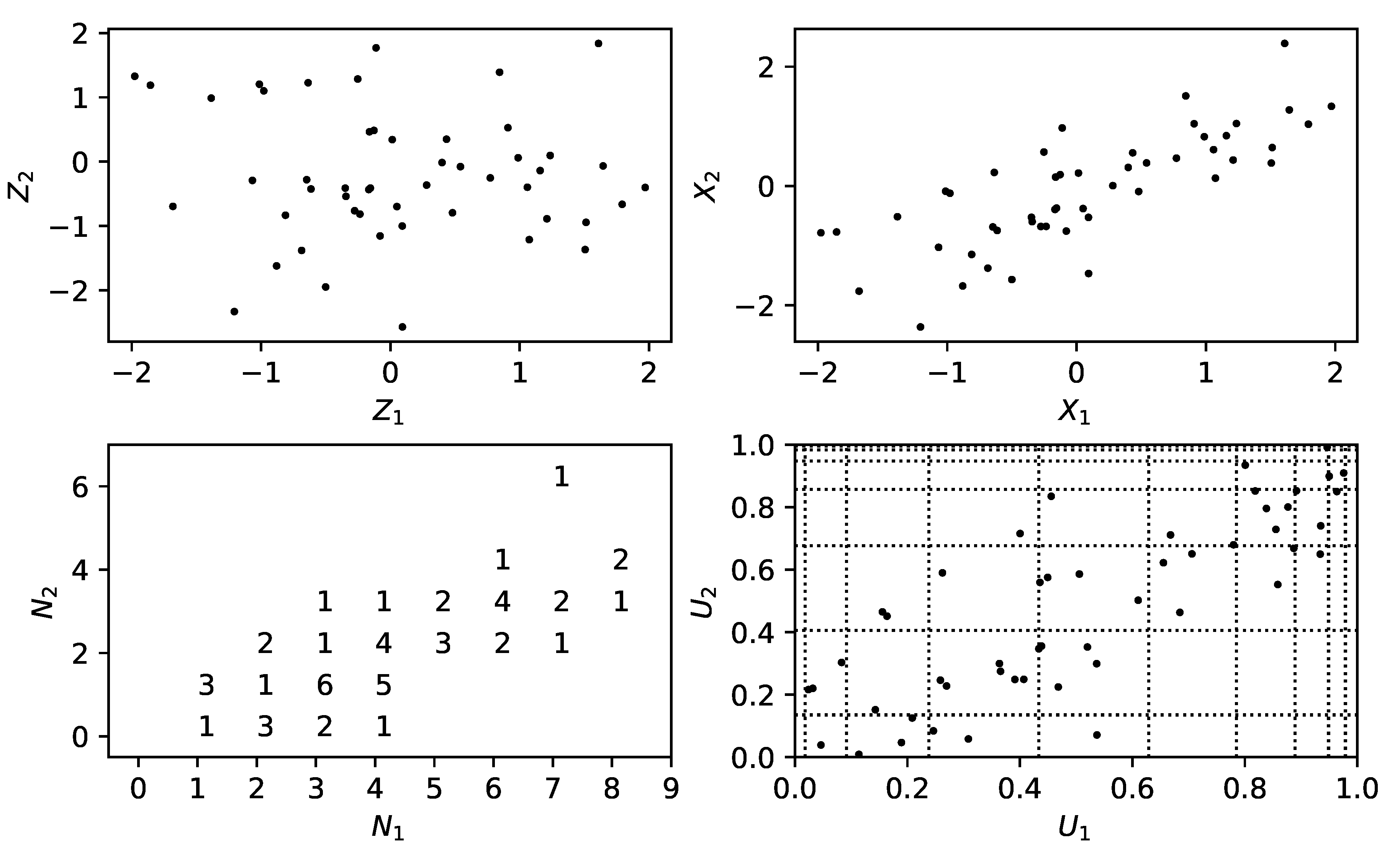
The method is as follows. Given a permissible correlation structure, to simulate a vector $(N_1,\dots ,N_J)$ of counts:

• Simulate a vector $(X_1,\dots ,X_J)$ of correlated, standard normal random variables. One can use the Cholesky decomposition of the correlation matrix to move from independent, standard normal random variables to such a correlated vector; see for instance Section 2.3.3 of Glasserman (2003).
• Transform these values to a dependent vector of uniform random variables $(U_1,\dots ,U_J)$. This can be done by setting each component as $U_j=\Phi (X_j)$ where $\Phi$ is the cumulative distribution function (CDF) of the standard normal distribution.
• The output $(N_1,\dots ,N_J)$ is given by setting each component to $F_j^{(-1)}(U_j)$, where $F_j^{-1}$ is the inverse of the $j^{th}$ Negative Binomial CDF1.

We note in passing that the key idea here is the Inverse Transform Method. The above method is illustrated in Figure 1 for two Poisson random variables.

We close this section by giving a result on the mean and variance of Equation (3), dropping the t for convenience, when we know the correlations between the $N_j$.

Proposition 2

(Mean and Variance of L). The mean and Variance of L are given by

$$\begin{array}{c}\hfill \mathbb{E}[L]=\sum _{j=1}^{J}E[N_j]E[X_1^j]\end{array}$$

(4)

and

$$\begin{array}{c}\hfill \begin{array}{cc}\hfill \mathrm{Var}(L)=& \sum _{j=1}^J\left\{\mathbb{E}[N_j]\mathrm{Var}(X_1^j)+\mathrm{Var}(N_j){\left(\mathbb{E}[X_1^j]\right)}^2\right\}\hfill \\ \hfill & +\sum _{i=1}^J\sum _{j=1,j\ne i}^J{\rho }_{ij}\mathbb{E}[X_1^i]\mathbb{E}[X_1^j]\sqrt{\mathrm{Var}(N_i)\mathrm{Var}(N_j)}\hfill \end{array}\end{array}$$

(5)

where ${\rho }_{ij}$ is the correlation between $N_i$ and $N_j$.

Proof. 

The expression for the mean of L comes from the independence of the counting processes and the severities, see for instance Proposition 2.2 of Shevchenko (2010). A similar expression for the variance of a random sum of random variables also exists in the same source, reading

$$\begin{array}{c}\hfill \mathrm{Var}(L_j)=\mathbb{E}[N_j]\mathrm{Var}(X_1^j)+\mathrm{Var}(N_j){\left(\mathbb{E}[X_1^j]\right)}^2\end{array}$$

However we cannot add these values up to get $\mathrm{Var}(L)$ because the $N_j$ are not independent. Rather we will start from

$$\begin{array}{c}\hfill \mathrm{Var}\left(\sum _{j=1}^J{L}_j\right)=\sum _{j=1}^J\mathrm{Var}(L_j)+\sum _{i=1}^J\sum _{j=1,j\ne i}^J\mathrm{Cov}(L_i,L_j)\end{array}$$

meaning that we also need to calculate the covariance terms for $i\ne j$. By definition we have

$$\begin{array}{c}\hfill \mathrm{Cov}(L_i,L_j)=\mathbb{E}[L_i{L}_j]-\mathbb{E}[L_i]\mathbb{E}[L_j]\end{array}$$

Given that we have the means to calculate expected values we can easily calculate the latter term. So we will focus on the first term, for $i\ne j$. We proceed by conditioning on the event $\{N_i=n_i,N_j=n_j\}$:

$$\begin{array}{cc}\hfill \mathbb{E}[L_i{L}_j|N_i=n_i,N_j=n_j]& =\mathbb{E}\left[\sum _{k=1}^{n_i}{X}_k^i·\sum _{l=1}^{n_j}{X}_l^j\right]\hfill \\ \hfill & =\mathbb{E}\left[\sum _{k=1}^{n_i}{X}_k^i\right]\mathbb{E}\left[\sum _{l=1}^{n_j}{X}_l^j\right]\hfill \\ \hfill & =n_i\mathbb{E}[X_k^i]n_j\mathbb{E}[X_1^j],\hfill \end{array}$$

where the second line comes from the independence of the different types of severity. Hence using iterated expectations we have

$$\begin{array}{cc}\hfill \mathbb{E}[L_i{L}_j]& =\mathbb{E}[\mathbb{E}[L_i{L}_j|N_i,N_j]]\hfill \\ \hfill & =\mathbb{E}[N_i\mathbb{E}[X_1^i]N_j\mathbb{E}[X_1^j]]\hfill \\ \hfill & =\mathbb{E}[X_1^i]\mathbb{E}[X_1^j]\mathbb{E}[N_i{N}_j]\hfill \end{array}$$

We can rearrange the formula for correlation ${\rho }_{ij}$ to give $\mathbb{E}[N_i{N}_j]$ in terms of ${\rho }_{ij}$:

$$\begin{array}{c}\hfill \mathbb{E}[N_i{N}_j]=\mathbb{E}[N_i]\mathbb{E}[N_j]+{\rho }_{ij}\sqrt{\mathrm{Var}(N_i)\mathrm{Var}(N_j)}\end{array}$$

Substituting backwards using the expression for $E[L_j]$, for $i\ne j$ we have

$$\begin{array}{cc}\mathrm{Cov}(L_i,L_j)\hfill & =\mathbb{E}[X_1^i]\mathbb{E}[X_1^j]\left(\mathbb{E}[N_i{N}_j]-\mathbb{E}[N_i]\mathbb{E}[N_j]\right)\hfill \\ \hfill & ={\rho }_{ij}\mathbb{E}[X_1^i]\mathbb{E}[X_1^j]\sqrt{\mathrm{Var}(N_i)\mathrm{Var}(N_j)}\hfill \end{array}$$

which gives the result. □

2.3. A Model for Mitigations

In the previous section we detailed a multivariate model for cybersecurity risk. This is valuable in and of itself because it can be used to describe risk, for instance by calculating a VaR value. However, we want to build on the key idea of Gordon and Loeb (2002) which is modelling the impact of mitigations on such risk. In this section we look at a simple model for mitigations.

We start by assuming that we have $m=1,\dots ,M$ different mitigations that each cost at most ${\omega }_m$ per year. We assume that we have an overall budget of z per year and denote the amount that we spend on each mitigation as $z_m$, with the restriction ${\sum }_{m=1}^M{z}_m\le z$ in one year. We fix a time horizon T of interest and assume that spending scales directly in T. That is, each mitigation costs at most ${\omega }_{m}T$ over $[0,T]$ and we have a budget of $zT$ over $[0,T]$. One could view the modelling in Gordon and Loeb (2002) as having one mitigation and one damage type and finding the best level of spending given different functional forms of $q(z_1)$, the probability of successful attack given spending on that mitigation. Mapping the mitigation models in Gordon and Loeb (2002) to our setting gives

$$\begin{array}{c}\hfill q(z)=\frac{q_0}{{(\alpha z+1)}^{\beta }}\end{array}$$

(6)

as well as

$$\begin{array}{c}\hfill q(z)=q_0^{\alpha z+1}\end{array}$$

(7)

where $q_0$ is the probability of successful attack in the absence of mitigations and $\alpha >0$ and $\beta \ge 1$ are parameters. Similar modelling, but with more than one mitigation and damage type, is done in Zhuo and Solak (2014). Here the effect of mitigations comes in through the expression for total losses as

$$\begin{array}{c}\hfill \sum _{s\in \mathcal{S}}\sum _{a\in \mathcal{A}}{f}_a{l}_{as}\left(\prod _{o\in \mathcal{O}}1-e_{oa}(z_o)\right)\end{array}$$

where $\mathcal{S},\mathcal{A}$ and $\mathcal{O}$ are sets of assets, attack types and mitigations, $f_a$ is a rate of attack, $l_{as}$ is the maximum damage from an attack and $e_{oa}(z_o)$ is the effectiveness of mitigation o on attack type a given spending $z_o$. This is given as

$$\begin{array}{c}\hfill e_{oa}(z_o)={\beta }_{oa}-e^{-({\alpha }_o{z}_o-ln{\beta }_{oa})}\end{array}$$

(8)

where ${\beta }_{oa}$ gives the maximal effectiveness of spending and ${\alpha }_o$ gives the rate at which spending approaches that level.

We use a multiplicative model similar to Zhuo and Solak (2014), but one that looks at frequency and severity separately. We first look at modelling the effect of spendings $\mathbf{z}=(z_1,\dots ,z_M)$ on the probability of success (and hence the frequency) of attack type j and then on the effect on severities.

The broad idea is that for each attack type j there is some baseline probability of success when there is no spending on mitigations, denoted $q_j^0$, and that the probability of successful attack goes down as spending increases. This is achieved by a factor that decreases linearly as spending increases to its maximum value ${\omega }_m$. Finally, the combined effect of all the mitigations is simply the product of those factors. Rather than model the effect of synergies or interference between mitigations as in Zhuo and Solak (2014), we use a floor value to ensure that this value does not become unrealistically small.

We will now fill in this broad idea. The linear reduction is achieved through a simple function f defined as

$$\begin{array}{c}\hfill f(z_m;s_m,e_m,{\omega }_m)=\left\{\begin{array}{cc}{s}_m+\frac{e_m-s_m}{{\omega }_m}{z}_m,& \mathrm{if}{z}_m\le {\omega }_m\\ e_m,& \mathrm{if}{z}_m>{\omega }_m\end{array}\right.\end{array}$$

(9)

This function describes a straight line between a start point $(0,s_m)$ and an end point $({\omega }_m,e_m)$ and a constant $e_m$ for any $z_m$ beyond ${\omega }_m$. We model the effect of spending $\mathbf{z}$ on the probability of a successful attack of type j over the period $[0,T]$ as

$$\begin{array}{c}\hfill q_j(\mathbf{z})=max\left(q_j^0\prod _{m=1}^{M}f(z_m;1,a_{mj},{\omega }_{m}T),\underline{q_j}\right)\end{array}$$

(10)

where $a_{mj}\in (0,1]$ is a factor that reduces $q_j^0$ if the full spending $z_m={\omega }_m$ is used and $\underline{q_j}$ is a floor on this probability. For example, $a_{mj}=1$ indicates no effect of mitigation m on the probability of success of attack type j and $a_{mj}=0$ indicates that the probability is reduced to 0. The interpretation of the expression for $q_j(\mathbf{z})$ is that the base probability of a successful attack of type j is modified by the product of different scaling factors, each coming from a different mitigation. The floor is used to ensure that the risk of attack does not become unrealistically small, as aforementioned.

A similar model is used for the effect of spending $\mathbf{z}$ on the severities. We assume that we know the distribution of severities $Y^j$ that apply in the absence of spending and model $X^j$ as a reduction of these values. That is, we set

$$\begin{array}{c}\hfill \begin{array}{cc}\hfill X_i^j=max(& Y_i^j\prod _{m=1}^{M}f(z_m;1,b_{mj},{\omega }_{m}T)+\sum _{m=1}^{M}f(z_m;0,c_{mj},{\omega }_{m}T),\underline{y_j})\hfill \end{array}\end{array}$$

(11)

Here, $b_{mj}\in (0,1]$ serves to scale $Y_i^j$, $c_{mj}<0$ represents a set reduction to every incident and $\underline{y_j}$ is a floor on the damage for this attack type. The interpretation of the above expressions is much as for the probability, but rather than only scaling damages includes the idea that a mitigation might give a set reduction to damage for each time an attack occurs.

There are several advantages to the above approach. Firstly, it allows for specific mitigations, rather than spending as a whole as in Gordon and Loeb (2002). Secondly, the form of f in Equation (9) means it is simple for estimates of the efficacy of mitigations to be translated into a model. That is, it is easier for the impact of a mitigation to be translated into parameters like $a_{mj},b_{mj}$ and $c_{mj}$ than it is to translate them into the parameters in Equations (6)–(8). Thirdly, as in the models in Gordon and Loeb (2002) and Zhuo and Solak (2014), the mitigating effect of spending z is modelled so that increased spending has diminishing effects. Fourthly and finally, the above approach allows for mitigations that affect frequency and severity of attacks separately.

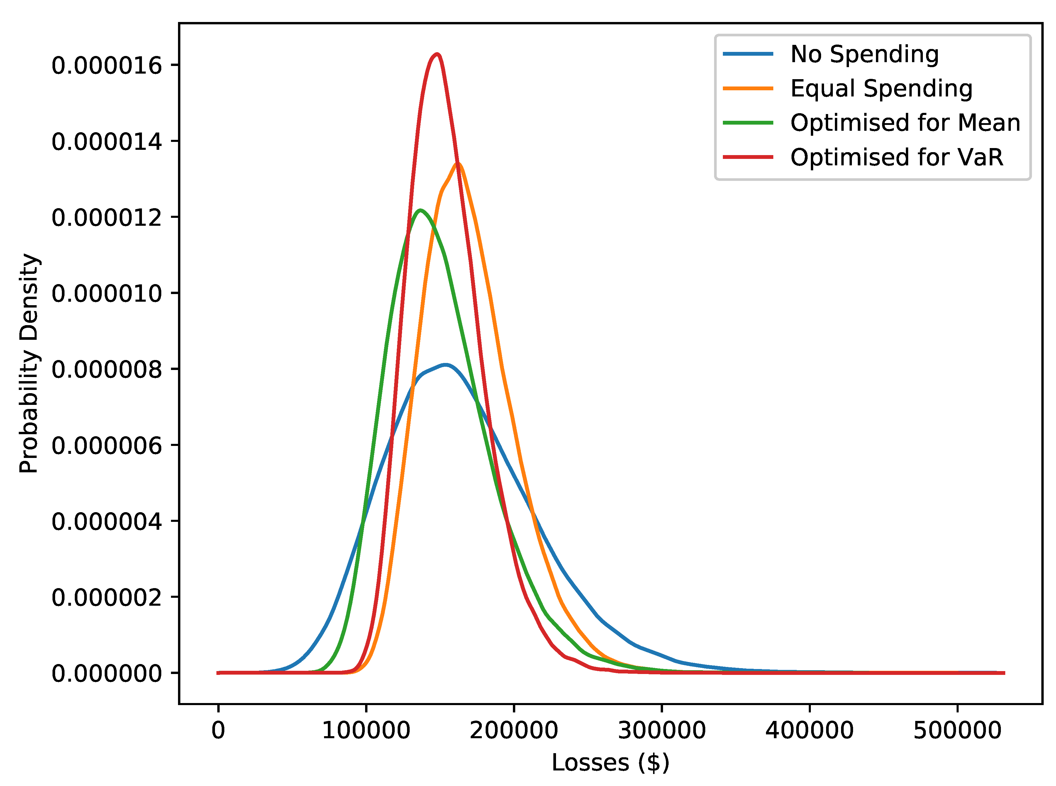
Giving a model for mitigations serves two purposes. Firstly, given assumptions on a given mitigation, one could see what losses might look like with and without that mitigation. This gives a means to judge whether the mitigation is worth implementing. Secondly, given a fixed budget, a specific objective (e.g., minimising the average of $L(t)$ or the VaR) and several possible mitigations, one can use numerical optimisation to choose the best choice of those mitigations.

We will look at the second idea in the Results section. A note on efficiency is worth making here. In numerically optimising to minimise the mean and VaR, a natural approach would be to use simulation. The problem with this approach is that every step of the optimisation routine would require many simulations. This would make the problem prohibitively expensive. Here we use the results of Proposition 2. While this gives the mean in closed form, it does not give the VaR. For this, we approximate the distribution of $L(t)$ by a Normal distribution with the mean and variance of $L(t)$. Given the inverse cumulative distribution function of the Normal distribution is easy to evaluate, we can find an approximation of the VaR.

Armed with a multivariate model for cybersecurity risk and a model for the impact of mitigations on the frequencies and severities, we look to apply this to real world data taken from Kuypers et al. (2016) and Paté-Cornell et al. (2018).

3. Results

In this section, we look at an application of the model to data from Kuypers et al. (2016) and Paté-Cornell et al. (2018).

3.1. Data

In these sources, the authors look at six years of tickets submitted by security engineers at a large, anonymous company that fall into different categories. The monthly counts of three of these categories (Data Spillage, Lost/Stolen and Malware) and the sum of all seven types (a category we will call All) are plotted as well as counts of incidents that take longer than certain times. We have used the data extraction software WebPlotDigitizer (Rohatgi 2018) to obtain estimates of this plotted data; in one case there are 63 of a total 72 months plotted, so the extracted datasets all have 63 entries. From the All category we create an artificial category called Other by subtracting the other series from it. This gives a total of four categories: Data Spillage, Lost/Stolen, Malware and Other.

The data gives two pieces of information. Firstly, for each category it gives the overall count of incidents each month. Secondly, it gives the number of incidents that took more than certain amounts of time to resolve in that month. The data that was extracted is given in the left hand column of Figure 2 and shown against simulated output of the fitted multivariate model, setting $T=1/12$.

Two points should be made. Firstly, the data being input is not in the purest sense real world data because one damage category has been constructed by us and further there are doubtless errors from the data extraction process. Secondly, the values relate to hours rather than dollars, which forces us to make assumptions on the costs per hour of each damage type and we will make these assumptions in non-specific “dollars”.

3.2. Quantifying Cyber Risks

The model is used to simulate losses three months into the future. A Kernel Density Estimate (KDE) of its density from 100,000 simulations is shown in Figure 3. This is one of the key outputs of the model and represents a quantitative description of Cyber security risk.

We next describe the assumptions underpinning the distribution of losses and the fitting of the data. The fit of the counts data (being the blue data in the left hand column of Figure 2) to a Negative Binomial distribution is done using the MASS library (Venables and Ripley 2002) and goodness of fit is tested by a chi squared test. The results are reported in

Table 1. Fit to Counts data. The columns $\widehat{r_j}$ and ${\mu }_j$ are returned by the numerical maximum likelihood estimation (with their standard errors) and $\widehat{p_j}$ is found by $\widehat{p_j}=\widehat{r_j}/(\widehat{{\mu }_j}+\widehat{r_j})$. The results of a chi squared test for goodness of fit of the Negative Binomial distribution to the counts data is also reported.

Damage Type j	$\widehat{{\mathit{r}}_{\mathit{j}}}$	$\widehat{{\mathit{\mu }}_{\mathit{j}}}$	$\widehat{{\mathit{p}}_{\mathit{j}}}$	p-Value
Data Spillage	6.057 (3.397)	3.19 (0.278)	0.665	0.66
Lost/Stolen	1.359 (0.236)	24.603 (2.731)	0.0523	$5.4\times {10}^{-5}$
Malware	4.941 (0.874)	193.921 (11.131)	0.0248	0.44
Other	2.494 (0.422)	343.635 (27.514)	0.00721	0.76

. While the use of this distribution is not rejected in three of the cases, the Lost/Stolen category is not well represented by a Negative Binomial distribution.

A plot of the Negative Binomial fits to the counts data is given in Figure 4. In particular we can see Lost / Stolen shows bimodality which explains why a Negative Binomial distribution is inappropriate.

Figure 2 and Figure 3 are based on several assumptions. These are gathered in

Table 2. Summary of assumptions on attacks. The $q_j^0$ are assumptions on the probability of successful attack in the absence of spending on mitigations. The parameters ${\alpha }_j$ and ${\beta }_j$ are found from $q_j^0$ and $\widehat{p_j}$ and $\widehat{r_j}$ in Table 1 using Equation (1). Finally, $\underline{y_j}$ is a floor on the amount of damage an attack can inflict and $\underline{q_j}$ is a floor on the probability of successful attack, as in Equations (10) and (11).

Damage Type j	${\mathit{q}}_{\mathit{j}}^{\mathbf{0}}$	${\mathit{\alpha }}_{\mathit{j}}$	${\mathit{\beta }}_{\mathit{j}}$	$\underline{{\mathit{y}}_{\mathit{j}}}$	$\underline{{\mathit{q}}_{\mathit{j}}}$	Cost/Hour
Data Spillage	0.9	6.057	0.142	0.500	0.05	350.0
Lost/Stolen	0.8	1.359	3.679 × ${10}^{-3}$	0.25	0.200	80.0
Malware	0.5	4.941	1.060 × ${10}^{-3}$	0.1	0.010	30.0
Other	0.8	2.494	4.835 × ${10}^{-4}$	0.05	0.100	20.0

. These assumptions are $q_j^0$ (the probability of a successful attack, with no spending on mitigations), $\underline{y_j}$ (the best case for the amount of time it will take to resolve an incident), $\underline{q_j}$ (the best case (lowest) probability of successful attack) and the costs per hour of resolving the different types of incident. These are dummy figures; they do not come from any specific research and, other than ensuring that data spillage has the highest cost, do not reflect any personal opinion on what these values should be.

The sample correlations between the counts are reported in

Table 3. The sample correlations between data sets ${\{N_i\}}_{j=1}^{T_j}$ and ${\{N_j\}}_{j=1}^{T_j}$. These are found by taking the total counts for each of the four categories (the blue lines in Figure 2) and finding the sample linear correlation between the different sets of counts.

	Data Spillage	Lost/Stolen	Malware	Other
Data Spillage	1	0.081	0.020	0.116
Lost/Stolen	-	1	−0.438	0.664
Malware	-	-	1	−0.103
Other	-	-	-	1

. The correlations in Table 3 are used to create a multivariate model for counts. One hundred simulations of this model are shown with the empirical counts in Figure 5.

We plot the survival functions (or complementary CDFs) of the severities for each category in Figure 6. These are constructed from the input data series in a simple way. First, for each hour h (20 and 50 for Data Spillage and 2, 5, 10 and 20 for the other categories), we calculate a value $S_j(h)$ by dividing the average of the number of incidents that took longer than h hours by the average number of all incidents; these values $S_j(h)$ are the red crosses in Figure 6. Then a survival function is interpolated (starting from (0,1)) through these points, extrapolating past the last point by using the gradient over the penultimate period.

3.3. Mitigating Cyber Risks

In this section we make some assumptions on mitigations and then optimise towards different objectives. A plot of the second key output of the model is in Figure 7, which shows density estimates of the losses after three months under different ways of spending a fixed budget of z = 300,000 dollars per year over a time period of three months, i.e., a budget of 75,000 dollars. The different ways of spending are: no spending on mitigations, spending equally on all possible mitigations, spending so as to minimise average loss and spending so as to minimise the 99% VaR.

Research and information on the quantitative effect of mitigations is very limited so we need to make assumptions. We loosely base our assumptions on the recommendations from the Australian Signals Directorate (The Australian Signals Directorate 2017). In particular, the recommendations in this source include relative, qualitative measures of expense and effectiveness. Otherwise, our assumptions are chosen to highlight the fact that optimising the model will give different output depending on the objective. We take five mitigations from The Australian Signals Directorate (2017). These mitigations and assumptions on their costs are listed in

Table 4. Names and maximum costs (per year) of different methods of mitigating cyber attack. These methods are taken from the Australian Signals Directorate The Australian Signals Directorate (2017). We follow the ordering of expenses given in this source, but the exact values are chosen for the sake of demonstrating the use of the model.

Mitigation Name	${\mathit{\omega }}_{\mathit{m}}$
Application Whitelisting	200,000
Patch Applications	200,000
Continuous Incident Detection	300,000
Antivirus Software	150,000
TLS Encryption	150,000

. Note that the level of the budget means that all measures cannot be purchased in full at the same time and that further the mitigation method Continuous Incident Detection is too expensive to afford in full.

Recall that the parameters $a_{mj},b_{mj}$ and $c_{mj}$ in Equations (10) and (11) detail the mitigations model; for mitigation m and attack type j, these lower the probability of successful attack, lower the amount of damage and give a fixed decrement to the amount of damage, respectively. Their assumed values are given in

Table 5. Values of $a_{mj},b_{mj}\in [0,1]$ and $c_{mj}\le 0$, each entry gives a triple $(a_{mj},b_{mj},c_{mj})$. A entry of ∗ means a default entry of $(1,1,0)$, meaning the mitigation has no effect on that attack type. Entries of the type $(a_{mj},\ast ,\ast )$ mean that the mitigation has an effect on $q_j$ but not on $Y_j$. For instance, the first row states that a full investment in Application Whitelisting reduces the probability of a successful Malware attack by a factor of $0.6$, reduces the relevant damage by a factor of $0.3$ and takes one hour off the resolution of each successful attack. The third row, first column states that Continuous Incident Detection reduces the probability and damage of a successful Data Spillage incident by a factor of $0.1$.

	Data Spillage	Lost/Stolen	Malware	Other
Application Whitelisting	*	*	(0.6,0.3,−1.0)	*
Patch Applications	*	*	*	(0.5,0.4,−0.5)
Continuous Incident Detection	(0.1,0.1,*)	(0.6,0.8,*)	*	*
Antivirus Software	*	*	(0.8,*,−1.0)	*
TLS Encryption	*	*	*	(0.8,*,−1.0)

.

We set $T=3/12$, rather than the one month of the input data. This means the available budget is 75,000 dollars over this period. Two optimisations are carried out: one to minimise $\mathbb{E}[L(T)+{\sum }_m{z}_m]$ and the other to minimise $min\{L_{*}>0:\mathbb{P}(L(T)+{\sum }_m{z}_m>L_{*})\le 0.01\}$. The purpose of adding the ${\sum }_m{z}_m$ term is to ensure that the costs of the mitigations are taken into account. The optimisations are done by the implementation of COBYLA given in the scipy library (Virtanen et al. 2020). In optimisation we use the result in Proposition 2 as described in the last part of Section 2.3. This compares to simulating to find the mean and VaR, which is what is done once the optimised choices are found in Figure 7 and

Table 6. The Average, VaR and % Spend of Budget for the four densities in Figure 7. The % reductions are from the “No Spend” case, the term in parenthesis represents an increase. The VaR terms are simulated, their errors going down are 0.9%, 0.6%, 0.8% and 0.6% respectively. Note that these values are inclusive of the budget spent, so in the bottom row the average amount of damages over the period is 79,664 dollars, with 75,000 dollars spent on mitigations bringing the losses up to 154,664 dollars.

Approach	$\mathbb{E}[\mathit{L}(\mathit{T})]$	% Reduction	VaR	% Reduction	% Spend
No Spend	164,653	0	306,626	0	0
Equal Spend	169,578	(2.99)	256,908	16.21	100.000
Optimise Mean	150,551	8.57	254,094	17.13	66.69
Optimise VaR	154,664	6.07	228,763	25.39	100.000

. Attempting an optimisation where each the objective function needs to be simulated at each step would be prohibitively expensive. The values of the mean and 99% VaR of $L(T)$ and the % spend of the available 75,000 dollars are given in Table 6.

The means and standard deviations of the $N_j(T)$ and $L_j(T)$ for $T=3/12$ are given in

Table 7. The averages and standard deviations of the frequency and total losses for each different type of damage. This table shows in particular how the assumptions on the cost of an incident map to costs over a three month period.

Damage Type j	$\mathbb{E}{[\mathit{N}}_{\mathit{j}}]$	$\mathbf{sd}{(\mathit{N}}_{\mathit{j}})$	$\mathbb{E}{[\mathit{L}}_{\mathit{j}}]$	$\mathbf{sd}{(\mathit{L}}_{\mathit{j}})$
Data Spillage	9.6	4.97	52,302	30,704
Lost/Stolen	73.9	63.95	14,801	13,026
Malware	582.9	263.33	60,057	27,257
Other	1032.7	654.07	37,493	23,858

.

The output of the optimisation procedure is the proportion of the available budget that should be spent on each type of mitigation. These are given in Figure 8 and compared to maximum possible spends. This is the second key output of the model. Given assumptions on mitigations, these give the amount of spending on the mitigations to achieve different objectives.

4. Discussion

In fitting the model to real world data, we can see it gives realistic output, gives a distribution of losses, allows for different types of attacks and mitigations, includes dependence, and has a mitigation model that can target frequency and losses separately. The model adds to the literature by improving the modelling of damages in Gordon and Loeb (2002) towards the sort of treatment in Sawik (2013), while being fitted to real world data.

Figure 2 shows that the model gives realistic output from real world input. It is of course not perfect. In particular, a Negative Binomial distribution for the counts of Lost/Stolen does not fit observed data. An implicit assumption of the model is that of stationarity, but the simulated output of Lost/Stolen looks rather different from the input. Of import is the log scale on the y-axis. The input data has a stationary period over the first 20 or so months, before trending upward. The scaling means that the input frequency is actually approximately exponentially increasing in time. These two periods can be seen in Figure 4 and lead to the poor fit. In contrast, the model implicitly assumes stationarity. That is, it assumes that the parameters of the frequencies and severities do not change over time. It is our view that the conclusions coming from the model do not suffer overall from this breached assumption. The use of a copula means that a different type of distribution could be used for this type of damage.

Of more concern is the distributions for severities. While in Kuypers et al. (2016) the choice is a Power law, we lack that more finely grained view of the data. A first approach was to fit a lognormal survival function to the points $S_j(h)$. This gave an overly light tail, which lead to the more empirical approach plotted in Figure 6. It is surprising that such a blunt approach leads to the reasonable output in Figure 2.

The first key output of the modelling is the distribution of losses, given in Figure 3. This gives a much more nuanced view of possible future losses than just the mean, which is what ALE is. In particular, it shows a relatively heavy right tail. An advantage to the model is that the time horizon of interest T is independent of the input data; we could just as easily change T to be six months or ten days.

Comparing the simulated pairwise counts in Figure 5 to the observed pairwise counts suggests the use of the Gaussian copula dependence structure being reasonable. It is not clear how much influence the correlations have on the final values. Proposition 2 shows that there will be no effect on the mean and that there will be an effect on the variance. Indeed, for this data and assumptions the variance of L increases by about 7% compared with the output when correlations are all set to 0, leaving all other values unchanged. One would think that this leads to a larger VaR, but simulated values are essentially equal. For this set of data and these assumptions, the dependence modelling has very little effect.

This is not entirely surprising, as we can only reject the null hypothesis of independence for the pairs Lost/Stolen / Malware and Lost/Stolen / Other. This does not support the view that a model with dependence is necessary. Nevertheless, our opinion is that some form of connection between the different categories is a necessary ingredient in a model for Cybersecurity risk.

One can test the importance of the input correlation matrix to the final VaR as follows. Using the method outlined in Rebonato and Jäckel (1999), simulate different correlation matrices. For each simulated matrix, calculate an overall measure of dependence as the average of the off-diagonal values. Finally, calculate the VaR for the simulated correlation matrix and compare it to the VaR that results with zero correlations by looking at the ratio of these two values. The outcome of 20,000 such simulations is given in Figure 9.

This image suggests that although the example data’s correlations have no effect, in extreme cases the correlation could move the VaR by as much as 30% over a model that has all components independent of one another.

While the model for losses is driven by the data, the model for mitigations is highly stylised. The aim is to give a framework by which cybersecurity experts could supply estimates of reductions in success and damage. While it is stylised, it includes the idea that mitigations might target frequency and severities separately, as well as having a weak interaction effect by assuming limits on the efficacy of mitigations. It is also designed to be easy to map from an expert’s opinion to parameters.

The fact that mitigations can target different types of attack means that different strategies for optimisation, either minimising the mean or the VaR, can be pursued. In Table 6, we establish a baseline by spending equally across all categories before optimising to minimise the mean and VaR. Spending equally in this manner decreases the VaR, but increases the average loss. Both of the average loss and VaR are reduced when looking at the other strategies. As would be expected, minimising the mean gives the lowest average loss and minimising the VaR gives the lowest VaR. The former strategy saves on average costs by leaving some of the budget unspent, where the later strategy spends this money to lower the VaR.

The assumptions are chosen so that there are solutions that the optimisation “should” find. One can see from Table 7 which types are most important. In particular, we can see from $\mathbb{E}[N_j]$ and $\mathbb{E}[L_j]$ that Data spillage is rare but damaging; this is due to the assumption on its cost per hour. From Table 5, we can see that only continuous incident detection makes this less frequent and less severe. We can also see that Application Whitelisting and Patch Applications are better at dealing with Malware and Other than Antivirus Software and TLS Encryption, although this needs to be balanced with their lower costs. All things being equal, one would expect a strategy to lower the VaR would focus on Continuous Incident Detection and would expect that Application Whitelisting and Patch Applications are preferred to Antivirus Software and TLS Encryption.

This is essentially what we see in Figure 8; both strategies focus on the more effective methods, with the VaR minimising approach spending the most overall. The optimisation is imperfect; because the Malware category is more damaging than the Other category, one would expect any money on the last two mitigations to be spent on Antivirus Software rather than TLS Encryption.

5. Conclusions

This paper looks firstly at describing a model to quantify losses from cybersecurity risk and then secondly at enhancing it with a model for mitigations to optimise towards certain goals. The important features of the model for losses are that it can account for several types of attack and for dependence between different types of attack. The important features of the model for mitigations are that it is simple and targets frequency and severity separately. The simplicity means that expert knowledge can be translated into the model.

The model can be used by practitioners and policy makers in two key ways. Firstly, it can be used to more exactly model potential losses from Cyber attacks. Secondly, given assumptions on the efficacy of different mitigation methods, it can be used to give the optimal choice of mitigations for a given objective.

The model can be extended in several ways. Firstly, VaR and the Gaussian copula are used for simplicity’s sake and more sophisticated risk measures (see, e.g., Artzner et al. 1999) and copulae exist. Secondly, the framework of the Common Shocks model from Lindskog and McNeil (2003), which allows for an incident of one type to cause another, would be a means to introduce a more realistic form of dependence. Thirdly and finally, it is unrealistic to imagine that fractional amounts of mitigations can be purchased. As mentioned in the Introduction, there is a collection of papers that use constraint programming which do not suffer from this issue.

There are two key concepts that this paper rests upon. The first is that it is important to model different types of attack and their dependence. In the numerical example considered here, the dependence modelling was of little consequence. However, the effect of changing the dependence structure could change estimates of risk by up to 30%. The second is that although data for the effect of mitigations on attacks is limited and this limits the modelling, it is worthwhile to optimise the choice of mitigations. In the numerical example considered here, the reduction in VaR is 25% rather than the 16% found from spending naïvely.

References

1. Artzner, Philippe, Freddy Delbaen, Jean-Marc Eber, and David Heath. 1999. Coherent measures of risk. Mathematical Finance 9: 203–28. [Google Scholar] [CrossRef]
2. Baskerville, Richard. 1991. Risk analysis: An interpretive feasibility tool in justifying information systems security. European Journal of Information Systems 1: 121–30. [Google Scholar] [CrossRef]
3. Bojanc, Rok, and Borka Jerman-Blažič. 2008. Towards a standard approach for quantifying an ict security investment. Computer Standards & Interfaces 30: 216–22. [Google Scholar]
4. Chavez-Demoulin, V., P. Embrechts, and J. Nešlehová. 2006. Quantitative models for operational risk: Extremes, dependence and aggregation. Journal of Banking and Finance 30: 2635–58. [Google Scholar] [CrossRef] [Green Version]
5. Eling, Martin, and Werner Schnell. 2016. Ten Key Questions on Cyber Risk and Cyber Risk Insurance. Technical Report. Geneva: The Geneva Association. [Google Scholar]
6. Geer, Daniel, Kevin Soo Hoo, and Andrew Jaquith. 2003. Information security: Why the future belongs to the quants. IEEE Security & Privacy 99: 24–31. [Google Scholar]
7. Genest, Christian, and Anne-Catherine Favre. 2007. Everything you always wanted to know about copula modeling but were afraid to ask. Journal of Hydrologic Engineering 12: 347–68. [Google Scholar] [CrossRef]
8. Glasserman, Paul. 2003. Monte Carlo Methods in Financial Engineering. New York: Springer. [Google Scholar]
9. Gordon, Lawrence A., and Martin P. Loeb. 2002. The economics of information security investment. ACM Transactions on Information and System Security 5: 438–57. [Google Scholar] [CrossRef]
10. Gurland, John. 1959. Some applications of the negative binomial and other contagious distributions. The American Journal of Public Health 49: 1388–99. [Google Scholar] [CrossRef] [PubMed] [Green Version]
11. Hubbard, Douglas W., and Richard Seiersen. 2016. How to Measure Anything in Cybersecurity Risk. Hoboken: John Wiley & Sons. [Google Scholar]
12. Hulthén, Rolf. 2009. Managing Information Risk and the Economics of Security. Chapter Communicating the Economic Value of Security Investments: Value at Security Risk. Boston: Springer, pp. 121–40. [Google Scholar]
13. Jacobson, Robert, William Brown, and Peter Browne. 1974. Guidelines for Automatic Data Processing, Physical Security and Risk Management; Technical Report FIPS PUB 31; Gaithersburg: National Bureau of Standards.
14. Kuypers, Marshall A., Thomas Maillart, and Elisabeth Paté-Cornell. 2016. An Empirical Analysis of Cyber Security Incidents at a Large Organization. Available online: https://fsi-live.s3.us-west-1.amazonaws.com/s3fs-public/kuypersweis_v7.pdf (accessed on 26 June 2017).
15. Lee, Yong Jick, Robert Kauffman, and Ryan Sougstad. 2011. Profit-maximizing firm investments in customer information security. Decision Support Systems 51: 904–20. [Google Scholar] [CrossRef]
16. Leslie, Nandi O., Richard E. Harang, Lawrence P. Knachel, and Alexander Kott. 2018. Statistical models for the number of successful cyber intrusions. Journal of Defense Modeling and Simulation: Applications, Methodology, Technology 15: 49–63. [Google Scholar] [CrossRef] [Green Version]
17. Lindskog, Filip, and Alexander J. McNeil. 2003. Common poisson shock models: Applications to insurance and credit risk modelling. ASTIN Bulletin 33: 209–38. [Google Scholar] [CrossRef] [Green Version]
18. Munteanu, Adrian. 2017. Running the risk IT—More perception and less probabilities in uncertain systems. Information & Computer Security 25: 345–54. [Google Scholar]
19. Nelsen, Roger B. 1999. An Introduction to Copulas. Lecture Notes in Statistics. New York: Springer. [Google Scholar]
20. Oppliger, Rolf. 2015. Quantitative risk analysis in information security management: A modern fairy tale. IEEE Security & Privacy 13: 18–21. [Google Scholar]
21. Paté-Cornell, M-Elisabeth, Marshall Kuypers, Matthew Smith, and Philip Keller. 2018. Cyber risk management for critical infrastructure: A risk analysis model and three case studies. Risk Analysis 38: 226–41. [Google Scholar] [CrossRef] [PubMed]
22. Rebonato, Riccardo, and Peter Jäckel. 1999. The most general methodology to create a valid correlation matrix for risk management and option pricing purposes. Available online: https://papers.ssrn.com/sol3/papers.cfm?abstract_id=1969689 (accessed on 31 August 2017).
23. Risk.net. 2020. Top 10 operational risks for 2020. March. Available online: https://www.risk.net/risk-management/7450731/top-10-operational-risks-for-2020 (accessed on 2 June 2020).
24. Rohatgi, Ankit. 2018. WebPlotDigitizer. January. Available online: https://automeris.io/WebPlotDigitizer (accessed on 19 March 2018).
25. Ross, Sheldon M. 2010. Introduction to Probability Models, 10th ed. Cambridge: Academic Press. [Google Scholar]
26. Sawik, Tadeusz. 2013. Selection of optimal countermeasure portfolio in IT security planning. Decision Support Systems 55: 156–64. [Google Scholar] [CrossRef]
27. Shevchenko, Pavel V. 2010. Calculation of aggregate loss distributions. The Journal of Operational Risk 5: 3–40. [Google Scholar] [CrossRef] [Green Version]
28. The Australian Signals Directorate. 2017. Strategies to Mitigate Cyber Security Incidents. Available online: https://www.cyber.gov.au/sites/default/files/2019-03/Mitigation_Strategies_2017.pdf (accessed on 1 February 2018).
29. Toscas, Peter, and Malcolm Faddy. 2003. Likelihood-based analysis of longitudinal count data using a generalized poisson model. Statistical Modelling 3: 99–108. [Google Scholar] [CrossRef]
30. Venables, W. N., and B. D. Ripley. 2002. Modern Applied Statistics with S, 4th ed. New York: Springer, ISBN 0-387-95457-0. [Google Scholar]
31. Viduto, Valentina, Carsten Maple, Wei Huang, and David López-Peréz. 2012. A novel risk assessment and optimisation model for a multi-objective network security countermeasure selection problem. Decision Support Systems 53: 599–610. [Google Scholar] [CrossRef] [Green Version]
32. Virtanen, Pauli, Ralf Gommers, Travis E. Oliphant, Matt Haberland, Tyler Reddy, David Cournapeau, Evgeni Burovski, Pearu Peterson, Warren Weckesser, Jonathon Bright, and et al. 2020. SciPy 1.0: Fundamental algorithms for scientific computing in Python. Nature Methods 17: 261–72. [Google Scholar] [CrossRef] [PubMed] [Green Version]
33. Wang, Jingguo. 2008. A value-at-risk approach to information security investment. Information Systems Research 19: 106–20. [Google Scholar] [CrossRef]
34. Zhuo, Yueran, and Senay Solak. 2014. Measuring and optimizing cybersecurity investments: A quantitative portfolio approach. Paper presented at the 2014 Industrial and Systems Engineering Research Conference, Montréal, QC, Canada, May 31–June 3. [Google Scholar]
1.
We note that there are some technicalities to inverting the distribution of a discrete random variable that we are glossing over.
Figure 1. Moving clockwise from the top left, the four plots show how to simulate 100 pairs ( N 1 , N 2 ) of Poisson random variables with λ 1 = 4.0 , λ 2 = 2.0 under a Gaussian copula with ρ = 0.8 . The top left hand plot shows 100 pairs of independent N ( 0 , 1 ) random variables ( Z 1 , Z 2 ) . In the top right hand plot these are mapped to correlated standard normal random variables ( X 1 , X 2 ) using the Cholesky decomposition of the covariance/correlation matrix. In the bottom right hand plot, these are mapped backwards to [ 0 , 1 ] 2 using the standard normal CDF to give correlated uniform random variables ( U 1 , U 2 ) . The dashed lines are from the PMF of the two Poisson random variables, which can be used in inverting the joint distribution. The final picture shows the simulated distribution; that is, the number of simulated outcomes of each pairing of N 1 and N 2 . As an example, because there are six points ( U 1 , U 2 ) that are in [ F N 1 ( 2 ) , F N 1 ( 3 ) ] × [ F N 2 ( 0 ) , F N 2 ( 1 ) ] there are six outcomes of { N 1 = 3 , N 2 = 1 } .
Risks 08 00061 g001
Figure 2. Left hand side: input data over 63 months, extracted from Kuypers et al. (2016) and Paté-Cornell et al. (2018). In each case, the blue line gives the total number of incidents in that month. The lines below the blue give the number of incidents that take more than 2, 5, 10 and 20 h (20 and 50 h for Data Spillage). Right hand side: corresponding output from simulations of the fitted model. Each month is independent of one another, but within a month the number of incidents is dependent.
Risks 08 00061 g002
Figure 3. Gaussian KDE estimates of losses three months into the future, constructed from 100,000 simulations with no spending on mitigation. The VaR at the α = 0.01 level is 306,626 dollars; the relevant part of the density is highlighted in red.
Risks 08 00061 g003
Figure 4. Histograms of observed counts for each category of damage with the PMF of the fitted Negative Binomial distribution overlaid in red (with lines between each point of the discrete function).
Risks 08 00061 g004
Figure 5. In black: the observed counts plotted against one another. In red: 100 simulated values of the counts under a Gaussian copula with the correlations given in Table 3.
Risks 08 00061 g005
Figure 6. In red are points found from averaging the data, interpolated in black are the survival functions used in the model.
Risks 08 00061 g006
Figure 7. Gaussian KDE estimates of losses under different ways of spending the budget, from 100,000 simulations of L ( T ) . The ways of spending are: no spending on mitigation, equal spending on each mitigation, spending chosen to minimise average losses and spending chosen to minimised VaR of the losses at the α = 0.01 level.
Risks 08 00061 g007
Figure 8. The output spendings for the five categories, from Application Whitelisting being 0 to Personnel Management as 4, after optimising to minimise the mean (in green) and to minimise the VaR at the α = 0.01 level (in red). The maximum spendings in black give the ratios ω m / z , the ratio of the cost of the mitigation to the available budget; this is the proportion of the budget needed to purchase this mitigation in full.
Risks 08 00061 g008
Figure 9. A total of 20,000 simulations of an approximation to the VaR found for a random correlation matrix divided by the VaR found when all correlations are set to 0. The ratio corresponding to the example data’s correlations is marked with a red cross and, being very near to 1.0, shows no real difference. In extreme cases the VaR is 30% larger or 30% smaller than the value that would come from setting correlations to be 0.
Risks 08 00061 g009