Assessing Asset-Liability Risk with Neural Networks

Abstract

We introduce a neural network approach for assessing the risk of a portfolio of assets and liabilities over a given time period. This requires a conditional valuation of the portfolio given the state of the world at a later time, a problem that is particularly challenging if the portfolio contains structured products or complex insurance contracts which do not admit closed form valuation formulas. We illustrate the method on different examples from banking and insurance. We focus on value-at-risk and expected shortfall, but the approach also works for other risk measures.

1. Introduction

Different financial risk management problems require an assessment of the risk of a portfolio of assets and liabilities over a given time period. Banks, mutual funds and hedge funds usually calculate value-at-risk numbers for different risks over a day, a week or longer time periods. Under Solvency II, insurance companies have to calculate one-year value-at-risk, whereas the Swiss Solvency Test demands a computation of one-year expected shortfall. A determination of these risk figures requires a conditional valuation of the portfolio given the state of the world at a later time, called risk horizon. This is particularly challenging if the portfolio contains structured products or complicated insurance policies which do not admit closed form valuation formulas. In theory, the problem can be approached with nested simulation, which is a two-stage procedure. In the outer stage, different scenarios are generated to model how the world could evolve until the risk horizon, whereas in the inner stage, cash flows occurring after the risk horizon are simulated to estimate the value of the portfolio conditionally on each scenario; see, e.g., Lee (1998), Glynn and Lee (2003), Gordy and Juneja (2008), Broadie et al. (2011) or Bauer et al. (2012). While nested simulation can be shown to converge for increasing sample sizes, it is often too time-consuming to be useful in practical applications. A more pragmatic alternative, usually used for short risk horizons, is the delta-gamma method, which approximates the portfolio loss with a second order Taylor polynomial; see, e.g., Rouvinez (1997), Britten-Jones and Schaefer (1999) or Duffie and Pan (2001). If first and second derivatives of the portfolio with respect to the underlying risk factors are accessible, the method is computationally efficient, but its accuracy depends on how well the second order Taylor polynomial approximates the true portfolio loss. Similarly, the replicating portfolio approach approximates future cashflows with a portfolio of liquid instruments that can be priced efficiently; see e.g., Wüthrich (2016), Pelsser and Schweizer (2016), Natolski and Werner (2017) or Cambou and Filipović (2018). Building on work on American option valuation (see e.g., Carriere 1996; Longstaff and Schwartz 2001; Tsitsiklis and Van Roy 2001), Broadie et al. (2015) as well as Ha and Bauer (2019) have proposed to regress future cash flows on finitely many basis functions depending on state variables known at the risk horizon. This gives good results in a number of applications. However, typically, for it to work well, the basis functions have to be chosen well-adapted to the problem.

In this paper we use a neural network approach to approximate the value of the portfolio at the risk horizon. Since our goal is to estimate tail risk measures such as value-at-risk and expected shortfall, we employ importance sampling when training the networks and estimating the risk figures. In addition, we try different regularization techniques and test the adequacy of the neural network approximations using the defining property of the conditional expectation. Neural networks have also been used for the calculation of solvency capital requirements by Hejazi and Jackson (2017), Fiore et al. (2018) and Castellani et al. (2019). But they all exclusively focus on value-at-risk, do not make use of importance sampling and apply neural networks in a slightly different way. Hejazi and Jackson (2017) develop a neural network interpolation scheme within a nested simulation framework. Fiore et al. (2018) and Castellani et al. (2019) both use reduced-size nested Monte Carlo to generate training samples for the calibration of the neural network. Here, we directly regress future cash-flows on a neural network without producing training samples.

The remainder of the paper is organized as follows. In Section 2, we set up the underlying risk model, introduce the importance sampling distributions we use in the implementation of our method and recall how value-at-risk and expected shortfall can be estimated from a finite sample of simulated losses. Section 3 discusses the training, validation and testing of our network approximation of the conditional valuation functional. In Section 4 we illustrate our approach on three typical risk calculation problems: the calculation of risk capital for a single put option, a portfolio of different call and put options and a variable annuity contract with guaranteed minimum income benefit. Section 5 concludes the paper.

2. Asset-Liability Risk

We denote the current time by 0 and are interested in the value of a portfolio of assets and liabilities at a given risk horizon $\tau >0$. Suppose all relevant events taking place until time $\tau$ are described by a d-dimensional random vector $X=(X_1,\cdots ,X_d)$ defined on a measurable space $(\mathsf{\Omega },\mathcal{F})$ that is equipped with two equivalent probability measures, $\mathbb{P}$ and $\mathbb{Q}$. We think of $\mathbb{P}$ as the real-world probability measure and use it for risk measurement. $\mathbb{Q}$ is a risk-neutral probability measure specifying the time-$\tau$ value of the portfolio through

$$V=v\left(X\right)+{\mathbb{E}}^{\mathbb{Q}}\left[\sum _{i=1}^I\frac{N_{\tau }}{N_{t_i}}{C}_{t_i}|X\right],$$

where v is a measurable function from ${\mathbb{R}}^d$ to $\mathbb{R}$ describing the part of the portfolio whose value is directly given by the underlying risk factors $X_1,\cdots ,X_d$; $C_{t_1},\cdots ,C_{t_I}$ are random cash flows occurring at times $\tau <t_1<\cdots <t_I$; and $N_{\tau },N_{t_1},\cdots ,N_{t_I}$ model the evolution of a numeraire process used for discounting.

Our goal is to compute $\rho \left(L\right)$ for a risk measure $\rho$ and the time $\tau$ net liability $L=-V$, which can be written as

$$L={\mathbb{E}}^{\mathbb{Q}}\left[Y\mid X\right]$$

for

$$Y=-v\left(X\right)-\sum _{i=1}^I\frac{N_{\tau }}{N_{t_i}}{C}_{t_i}.$$

Our approach works for a wide class of risk measures $\rho$. But for the sake of concreteness, we concentrate on value-at-risk and expected shortfall. We follow the convention of McNeil et al. (2015) and define value-at-risk at a level $\alpha \in (0,1)$, such as $0.95$, $0.99$ or $0.995$, as the left $\alpha$-quantile

$${\mathrm{VaR}}_{\alpha }\left(L\right):=min\left\{x\in \mathbb{R}:\mathbb{P}[L\le x]\ge \alpha \right\}=sup\left\{x\in \mathbb{R}:\mathbb{P}[L\ge x]>1-\alpha \right\}$$

(1)

and expected shortfall as

$${\mathrm{ES}}_{\alpha }\left(L\right):=\frac{1}{1-\alpha }{\int }_{\alpha }^1{\mathrm{VaR}}_u\left(L\right)du.$$

(2)

There exist different definitions of VaR and ES in the literature. But if the distribution function $F_L$ of L is continuous and strictly increasing, they are all equivalent1.

2.1. Conditional Expectations as Minimizing Functions

Let $\mathbb{P}\otimes \mathbb{Q}$ be the probability measure on $\mathcal{F}$ given by

$$\mathbb{P}\otimes \mathbb{Q}\left[A\right]:={\int }_{{\mathbb{R}}^d}\mathbb{Q}[A\mid X=x]\pi \left(dx\right),$$

where $\pi$ is the distribution of X under $\mathbb{P}$ and $\mathbb{Q}[A\mid X=x]$ is a regular conditional version of $\mathbb{Q}$ given X. We assume that Y belongs to $L^2(\mathsf{\Omega },\mathcal{F},\mathbb{P}\otimes \mathbb{Q})$. Then L is of the form $L=l\left(X\right)$ for a measurable function $l:{\mathbb{R}}^d\to \mathbb{R}$ minimizing the mean squared distance

$${\mathbb{E}}^{\mathbb{P}\otimes \mathbb{Q}}\left[{\left(l\left(X\right)-Y\right)}^2\right];$$

(3)

see, e.g., Bru and Heinich (1985). Note that l minimizes (3) if and only if

$$l\left(x\right)=\underset{u\in \mathbb{R}}{arg\; min}{\int }_{\mathbb{R}}{(u-y)}^2\mathbb{Q}[Y\in dy\mid X=x]\mathrm{for} \pi -\mathrm{almost} \mathrm{all} x\in {\mathbb{R}}^d,$$

where $\mathbb{Q}[Y\in dy\mid X=x]$ is a regular conditional $\mathbb{Q}$-distribution of Y given X. This shows that l is unique up to $\pi$-almost sure equality and can alternatively be characterized by

$$l\left(x\right)=\underset{u\in \mathbb{R}}{arg\; min}{\int }_{\mathbb{R}}{(u-y)}^2\mathbb{Q}[Y\in dy\mid X=x]\mathrm{for} \nu -\mathrm{almost} \mathrm{all} x\in {\mathbb{R}}^d$$

for any probability measure $\nu$ on ${\mathbb{R}}^d$ that is equivalent to $\pi$. In particular, if  ${\mathbb{P}}^{\nu }$ is the probability measure on $\sigma \left(X\right)$ under which X has distribution $\nu$, and Y is in $L^2(\mathsf{\Omega },\mathcal{F},{\mathbb{P}}^{\nu }\otimes \mathbb{Q})$, then l can be determined by minimizing

$${\mathbb{E}}^{{\mathbb{P}}^{\nu }\otimes \mathbb{Q}}\left[{\left(l\left(X\right)-Y\right)}^2\right]$$

(4)

instead of (3). Since we are going to approximate the expectation (4) with averages of Monte Carlo samples, this will give us some flexibility in simulating $(X,Y)$.

2.2. Monte Carlo Estimation of Value-at-Risk and Expected Shortfall

Let $X^1,\cdots ,X^n$ be independent $\mathbb{P}$-simulations of X. By $X^{\left(1\right)},\cdots ,X^{\left(n\right)}$ we denote the same sample reordered so that

$$L^{\left(1\right)}=l\left(X^{\left(1\right)}\right)\ge \cdots \ge L^{\left(n\right)}=l\left(X^{\left(n\right)}\right).$$

To obtain $\mathbb{P}$-simulation estimates of ${\mathrm{VaR}}_{\alpha }\left(L\right)$ and ${\mathrm{ES}}_{\alpha }\left(L\right)$, we apply the VaR and ES definitions (1)–(2) to the empirical measure $\frac{1}{n}{\sum }_{i=1}^n{\delta }_{L^{\left(i\right)}}$. This yields

$${\widehat{\mathrm{VaR}}}_{\alpha }\left(n\right):=L^{\left(j\right)}\mathrm{and}{\widehat{\mathrm{ES}}}_{\alpha }\left(n\right):=\frac{1}{1-\alpha }\sum _{i=1}^{j-1}\frac{L^{\left(i\right)}}{n}+\left(1-\frac{j-1}{(1-\alpha )n}\right)L^{\left(j\right)},$$

(5)

where

$$j=min\left\{i\in \left\{1,\cdots ,n\right\}:i/n>1-\alpha \right\};$$

see also McNeil et al. (2015). It is well known that if $F_L$ is differentiable at ${\mathrm{VaR}}_{\alpha }\left(L\right)$ with $F_L^{\prime }\left({\mathrm{VaR}}_{\alpha }\left(L\right)\right)>0$, then ${\widehat{\mathrm{VaR}}}_{\alpha }\left(n\right)$ is an asymptotically normal consistent estimator of order $n^{-1/2}$; see, e.g., David and Nagaraja (2003). If in addition, L is square-integrable, the same is true for ${\widehat{\mathrm{ES}}}_{\alpha }\left(n\right)$; see Zwingmann and Holzmann (2016).

2.3. Importance Sampling

Assume now that X is of the form $X=h\left(Z\right)$ for a transformation $h:{\mathbb{R}}^k\to {\mathbb{R}}^d$ and a k-dimensional random vector Z with density $f:{\mathbb{R}}^k\to {\mathbb{R}}_{+}$. To give more weight to important outcomes, we introduce a second density g on ${\mathbb{R}}^k$ satisfying $g\left(z\right)>0$ for all $z\in {\mathbb{R}}^k$, where $f\left(z\right)>0$. Let $Z^g$ be a k-dimensional random vector with density g and $Z^{g,1},\cdots ,Z^{g,n}$ independent simulations of $Z^g$. We reorder the simulations such that

$$L^{g,\left(1\right)}=l\circ h\left(Z^{g,\left(1\right)}\right)\ge \cdots \ge L^{g,\left(n\right)}=l\circ h\left(Z^{g,\left(n\right)}\right)$$

and consider the random weights

$$w^{\left(i\right)}=\frac{f\left(Z^{g,\left(i\right)}\right)}{ng\left(Z^{g,\left(i\right)}\right)}.$$

Since $f\left(Z^g\right)/g\left(Z^g\right)$ is integrable, one obtains from the law of large numbers that for every threshold $x\in \mathbb{R}$,

$$\sum _{i=1}^n{1}_{\left\{l\circ h\left(Z^{g,\left(i\right)}\right)\ge x\right\}}{w}^{\left(i\right)}$$

(6)

is an unbiased consistent estimator of the exceedance probability

$$\mathbb{P}[L\ge x]=\mathbb{P}\left[l\circ h\left(Z\right)\ge x\right]=\mathbb{E}\left[1_{\left\{l\circ h\left(Z^g\right)\ge x\right\}}\frac{f\left(Z^g\right)}{g\left(Z^g\right)}\right].$$

If in addition, g can be chosen so that $f\left(Z^g\right)/g\left(Z^g\right)$ is square-integrable, it follows from the central limit theorem that (6) is asymptotically normal with a standard deviation of order $n^{-1/2}$. In any case, ${\sum }_{i=1}^n{w}^{\left(i\right)}$ converges to 1 and the random measure ${\sum }_{i=1}^n{w}^{\left(i\right)}{\delta }_{l\circ h\left(Z^{g,\left(i\right)}\right)}$ approximates the distribution of L. Accordingly, we adapt the $\mathbb{P}$-simulation estimators (5) by replacing $i/n$ with ${\sum }_{m=1}^i{w}^{\left(m\right)}$. This yields the g-simulation estimates

$${\widehat{\mathrm{VaR}}}_{\alpha }^g\left(n\right):=L^{g,\left(j\right)}\mathrm{and}{\widehat{\mathrm{ES}}}_{\alpha }^g\left(n\right):=\frac{1}{1-\alpha }\sum _{i=1}^{j-1}{w}^{\left(i\right)}{L}^{g,\left(i\right)}+\left(1-\frac{1}{1-\alpha }\sum _{i=1}^{j-1}{w}^{\left(i\right)}\right)L^{g,\left(j\right)},$$

where

$$j=min\left\{i\in \left\{1,\cdots ,n\right\}:\sum _{m=1}^i{w}^{\left(m\right)}>1-\alpha \right\}.$$

If the $\alpha$-quantile $l_{\alpha }$ of $L=l\circ h\left(Z\right)$ were known, the exceedance probability $\mathbb{P}\left[L\ge l_{\alpha }\right]$ could be estimated by means of (6) with $x=l_{\alpha }$. To make the procedure efficient, one would try to find a density g on ${\mathbb{R}}^k$ from which it is easy to sample and such that the variance

$$\mathrm{Var}\left(1_{\left\{l\circ h\left(Z^g\right)\ge l_{\alpha }\right\}}\frac{f\left(Z^g\right)}{g\left(Z^g\right)}\right)=\mathbb{E}\left[1_{\left\{l\circ h\left(Z^g\right)\ge l_{\alpha }\right\}}\frac{f{\left(Z^g\right)}^2}{g{\left(Z^g\right)}^2}\right]-\mathbb{E}{\left[1_{\left\{l\circ h\left(Z^g\right)\ge l_{\alpha }\right\}}\frac{f\left(Z^g\right)}{g\left(Z^g\right)}\right]}^2,$$

becomes as small as possible. Since

$$\mathbb{E}\left[1_{\left\{l\circ h\left(Z^g\right)\ge l_{\alpha }\right\}}\frac{f\left(Z^g\right)}{g\left(Z^g\right)}\right]=\mathbb{E}\left[1_{\left\{l\circ h\left(Z\right)\ge l_{\alpha }\right\}}\right]=\mathbb{P}[L\ge l_{\alpha }]$$

does not depend on g, it can be seen that g is a good importance sampling (IS) density if

$$\mathbb{E}\left[1_{\left\{l\circ h\left(Z^g\right)\ge l_{\alpha }\right\}}\frac{f{\left(Z^g\right)}^2}{g{\left(Z^g\right)}^2}\right]=\mathbb{E}\left[1_{\left\{l\circ h\left(Z\right)\ge l_{\alpha }\right\}}\frac{f\left(Z\right)}{g\left(Z\right)}\right]$$

(7)

is small. We use the same criterion as a basis to find a good IS density for estimating ${\mathrm{VaR}}_{\alpha }$ and ${\mathrm{ES}}_{\alpha }$; see, e.g., Glasserman (2003) for more background on importance sampling.

2.4. The Case of an Underlying Multivariate Normal Distribution

In many applications X can be modelled as a deterministic transformation of a random vector with a multivariate normal distribution. Examples are included in Section 4 below. In this case, it can be written as

$$X=u\left(AZ\right)$$

(8)

for a function $u:{\mathbb{R}}^p\to {\mathbb{R}}^d$, a $p\times k$-matrix A and a k-dimensional random vector Z with a standard normal density f. To keep the problem tractable, we look for a suitable IS density g in the class of $N_k(m,I_k)$-densities $f_m$ with different mean vectors $m\in {\mathbb{R}}^k$ and covariance matrix equal to the k-dimensional identity matrix $I_k$. To determine a good choice of m, let $v\in {\mathbb{R}}^p$ be the vector with components

$$v_i=\left\{\begin{array}{cc}1\hfill & \mathrm{if} l\circ u \mathrm{is} \mathrm{increasing} in y_i\hfill \\ -1\hfill & \mathrm{if} l\circ u \mathrm{is} \mathrm{decreasing} in y_i\hfill \\ 0\hfill & \mathrm{else}.\hfill \end{array}\right.$$

If $A^{T}v=0$, we choose $m=0$. Otherwise, $v^{T}AZ/{\parallel A^{T}v\parallel }_2$ is standard normal. Denote its $\alpha$-quantile by $z_{\alpha }$. Then Z falls into the region

$$D=\left\{z\in {\mathbb{R}}^k:v^{T}Az/{\parallel A^{T}v\parallel }_2\ge z_{\alpha }\right\}$$

with probability $1-\alpha$, and $l\circ u\left(Az\right)$ tends to be large for $z\in D$. We choose m as the maximizer of $f\left(z\right)$ subject to $z\in D$, which leads to

$$m=\frac{A^{T}v}{\parallel A^T{v\parallel }_2}{z}_{\alpha }.$$

It is easy to see that this yields

$$f\left(z\right)<f_m\left(z\right)\mathrm{for} \mathrm{all} z\in D.$$

So, if D is sufficiently similar to the region $\left\{z\in {\mathbb{R}}^k:l\circ u\left(Az\right)\ge l_{\alpha }\right\}$, it can be seen from (7) that this choice of IS density will yield a reduction in variance.

3. Neural Network Approximation

Usually, the distribution of the risk factor vector X is assumed to be known. For instance, in all our examples in Section 4, they are of the form (8). On the other hand, in many real-world applications, there is no closed form expression for the loss function $l:{\mathbb{R}}^d\to \mathbb{R}$ mapping X to L. Therefore, we approximate $L=l\left(X\right)$ with $l^{\theta }\left(X\right)$ for a neural network $l^{\theta }:{\mathbb{R}}^d\to \mathbb{R}$; see e.g., Goodfellow et al. (2016). We concentrate on feedforward neural networks of the form

$$l^{\theta }=\psi \circ a_J^{\theta }\circ \phi \circ a_J^{\theta }\circ \cdots \circ \phi \circ a_1^{\theta },$$

where

• $q_0=d$, $q_J=1$, and $q_1,\cdots ,q_{J-1}$ are the numbers of nodes in the hidden layers $1,\cdots ,J-1;$
• $a_j^{\theta }$ are affine functions of the form $a_j^{\theta }\left(x\right)=A_{j}x+b_j$ for matrices $A_j\in {\mathbb{R}}^{q_j\times q_{j-1}}$ and vectors $b_j\in {\mathbb{R}}^{q_j},$ for $j=1,\dots ,J;$
• $\phi$ is a non-linear activation function used in the hidden layers and applied component-wise. In the examples in Section 4 we choose $\phi =tanh;$
• $\psi$ is the final activation function. For a portfolio of assets and liabilities a natural choice is $\psi =id$. To keep the presentation simple, we will consider pure liability portfolios with loss $L>0$ in all our examples below. Accordingly, we choose $\psi =exp$.

The parameter vector $\theta$ consists of the components of the matrices $A_j$ and vectors $b_j$, $j=1,\cdots ,J$. So it lives in ${\mathbb{R}}^q$ for $q={\sum }_{j=1}^J{q}_j(q_{j-1}+1)$. It remains to determine the architecture of the network (that is, J and $q_1,\cdots ,q_{J-1}$) and to calibrate $\theta \in {\mathbb{R}}^q$. Then VaR and ES figures can be estimated as described in Section 2 by simulating $l^{\theta }\left(X\right)$.

3.1. Training and Validation

In a first step we take the network architecture (J and $q_1,\cdots ,q_{J-1})$ as given and try to find a minimizer of $\theta \mapsto \mathbb{E}\left[{(l^{\theta }\left(X\right)-Y)}^2\right]$, where the expectation is either with respect to $\mathbb{P}\otimes \mathbb{Q}$ or ${\mathbb{P}}^{\nu }\otimes \mathbb{Q}$ for an IS distribution $\nu$ on ${\mathbb{R}}^d$. To do that we simulate realizations $(X^m,Y^m)$, $m=1,\cdots ,M_1+M_2$, of $(X,Y)$ under the corresponding distribution. The first $M_1$ simulations are used for training and the other $M_2$ for validation. More precisely, we employ a stochastic gradient descent method to minimize the Monte Carlo approximation based on the training samples

$$\frac{1}{M_1}\sum _{m=1}^{M_1}{\left(l^{\theta }\left(X^m\right)-Y^m\right)}^2$$

(9)

of $\mathbb{E}\left[(l^{\theta }\left(X\right)-Y)\right]$. At the same time we use the validation samples to check whether

$$\frac{1}{M_2}\sum _{m=M_1+1}^{M_1+M_2}{\left(l^{\theta }\left(X^m\right)-Y^m\right)}^2$$

(10)

is decreasing as we are updating $\theta$.

3.1.1. Regularization through Tree Structures

If the number q of parameters is large, one needs to be careful not to overfit the neural network. For instance, in the extreme case, the  network could be so flexible that it can bring (9) down to zero even in cases where the true conditional expectation $l\left(X\right)={\mathbb{E}}^{\mathbb{Q}}[Y\mid X]$ is not equal to Y. To prevent this, one can generate the training samples by first simulating $N_1$ realizations $X^i$ of X and then for every $X^i$, drawing $N_2$ simulations $Y^{i,j}$ from the conditional distribution of Y given $X^i$. In the simple example of Section 4.1, we chose $N_2=1$. In Section 4.2 and Section 4.3 we used $N_2=5$.

3.1.2. Stochastic Gradient Descent

In principle, one can use any numerical method to minimize (9). But  stochastic gradient descent methods have proven to work well for neural networks. We refer to  Ruder (2016) for an overview of different (stochastic) gradient descent algorithms. Here, we randomly2 split the $M_1$ training samples into b mini-batches of size B. Then we update $\theta$ based on the $\theta$-gradients of

$$\frac{1}{B}\sum _{m=(i-1)B+1}^{iB}{\left(l^{\theta }\left(X^m\right)-Y^m\right)}^2,i=1,\cdots ,b.$$

We use batch normalization and Adam updating with the default values from TensorFlow.

After b gradient steps, all of the training data have been used once and the first epoch is complete. For further epochs, we reshuffle the training data, form new mini-batches and perform b more gradient steps. The procedure is repeated until the training error (9) stops to decrease or the validation error (10) starts to increase.

3.1.3. Initialization

We follow standard practice and initialize the parameters of the network randomly. The final operation of the network is

$$x\mapsto \psi (A_{J}x+b_J).$$

Since the network tries to approximate Y, and in all our examples below we use $\psi =exp$, we initialize the last bias as

$$b_J^0=log\left(\frac{1}{M_1}\sum _{m=1}^{M_1}{Y}^m\right).$$

For the other parameters we use Xavier initialization; see Glorot and Bengio (2010).

3.2. Backtesting the Network Approximation

After having determined an approximate minimizer $\theta \in {\mathbb{R}}^q$ for a given network architecture, one can test the adequacy of the approximation $l^{\theta }\left(X\right)$ of the true conditional expectation $l\left(X\right)={\mathbb{E}}^{\mathbb{Q}}[Y\mid X]$. The quality of the approximation depends on different aspects:

(i)

Generalization error:

The true conditional expectation ${\mathbb{E}}^{\mathbb{Q}}\left[Y\mid X\right]$ is of the form $l\left(X\right)$ for the unique3 measurable function $l:{\mathbb{R}}^d\to \mathbb{R}$ minimizing the mean squared distance $\mathbb{E}\left[{\left(l\left(X\right)-Y\right)}^2\right]$. To approximate l we choose a network architecture and try to find a $\theta \in {\mathbb{R}}^q$ that minimizes the empirical squared distance

$$\frac{1}{M_1}\sum _{m=1}^{M_1}{\left(l^{\theta }\left(X^m\right)-Y^m\right)}^2.$$

(11)

But if the samples $(X^m,Y^m),$$m=1,\cdots ,M_1$, do not represent the distribution of $(X,Y)$ well, (11) might not be a good approximation of the true expectation $\mathbb{E}\left[{\left(l^{\theta }\left(X\right)-Y\right)}^2\right]$.

(ii)

Numerical minimization method:

The minimization of (11) usually is a complex problem, and one has to employ a numerical method to find an approximate solution $\theta$. The  quality of $l^{\theta }\left(X\right)$ will depend on the performance of the numerical method being used.

(iii)

Network architecture:

It is well known that feedforward neural networks with one hidden layer have the universal approximation property; see, e.g., Cybenko (1989); Hornik et al. (1989) or Leshno et al. (1993). That is, they can approximate any continuous function uniformly on compacts to any degree of accuracy if the activation function is of a suitable form and the hidden layers contain sufficiently many nodes. As a consequence, $\mathbb{E}\left[{(l^{\theta }\left(X\right)-l\left(X\right))}^2\right]$ can be made arbitrarily small if the hidden layer is large enough and $\theta$ is chosen appropriately. However, we do not know in advance how many nodes we need. And moreover, feedforward neural networks with two or more hidden layers have shown to yield better results in different applications.

Since we simulate from an underlying model, we are able to choose the size $M_1$ of the training sample large and train extensively. In addition, for any given network architecture, we also evaluate the empirical squared distance (11) on the validation set $(X^m,Y^m)$, $m=M_1+1,\cdots ,M_2$. So we suppose the generalization error is small and our numerical method finds a good approximate minimizer $\theta$ of (11). However, since we do not know whether a given network architecture is flexible enough to provide a good approximation to the true loss function l, we test for each trained network whether it satisfies the defining properties of a conditional expectation.

The loss function $l:{\mathbb{R}}^d\to \mathbb{R}$ is characterized by

$$\mathbb{E}\left[l\right(X\left)\xi \right(X\left)\right]=\mathbb{E}\left[Y\xi \right(X\left)\right]$$

(12)

for all measurable functions $\xi :{\mathbb{R}}^d\to \mathbb{R}$ such that $Y\xi \left(X\right)$ is integrable. Ideally, we would like $l^{\theta }$ to satisfy the same condition. But there will be an approximation error, and (12) cannot be checked for all measurable functions $\xi :{\mathbb{R}}^d\to \mathbb{R}$ satisfying the integrability condition. Therefore, we select finitely many measurable subsets $B_i\subseteq {\mathbb{R}}^d$, $i=1,\cdots ,I$. Then we generate $M_3$ more samples $(X^m,Y^m)$ of $(X,Y)$ and test whether the differences

(a)

${\sum }_{m=M_2+1}^{M_1+M_2+M_3}\left(l^{\theta }\left(X^m\right)-Y^m\right)/M_3$

(b)

${\sum }_{m=M_2+1}^{M_1+M_2+M_3}\left(l^{\theta }\left(X^m\right)-Y^m\right)l^{\theta }\left(X^m\right)/M_3$

(c)

${\sum }_{m=M_2+1}^{M_1+M_2+M_3}\left(l^{\theta }\left(X^m\right)-Y^m\right)1_{B_i}\left(X^m\right)/M_3$

are sufficiently close to zero. If this is not the case, we change the network architecture and train again.

4. Examples

As examples, we study three different risk assessment problems from banking and insurance. For comparison we generated realizations $(X^m,Y^m)$ of $(X,Y)$ under $\mathbb{P}\otimes \mathbb{Q}$ as well as ${\mathbb{P}}^{\nu }\otimes \mathbb{Q}$, where $\nu$ is the IS distribution on ${\mathbb{R}}^d$ obtained by changing the distribution of X. In all our examples, X has a transformed normal distribution as in Section 2.4. In each case we used 1.5 million simulations with mini-batches of size 10,000 for training, 500,000 simulations for validation and 500,000 for backtesting. After training and testing the network, we simulated another 500,000 realizations of X, once under $\mathbb{P}$ and then under ${\mathbb{P}}^{\nu }$, to estimate ${\mathrm{VaR}}_{99.5\%}\left(L\right)$ and ${\mathrm{ES}}_{99\%}\left(L\right)$.

We implemented the algorithms in Python. To train the networks we used the TensorFlow package.

4.1. Single Put Option

As a first example, we consider a liability consisting of a single put option with strike price $K=100$ and maturity $T=1/3$ on an underlying asset starting from $s_0=100$ and evolving according to

$$d{S}_t=\mu S_{t}dt+\sigma S_{t}d{W}_t^{\mathbb{P}}=r{S}_{t}dt+\sigma S_{t}d{W}_t^{\mathbb{Q}}$$

for an interest rate $r=1\%$, a drift $\mu =5\%$, a volatility $\sigma =20\%$, a $\mathbb{P}$-Brownian motion $W^{\mathbb{P}}$ and a $\mathbb{Q}$-Brownian motion $W^{\mathbb{Q}}$. As risk horizon we choose $\tau =1/52$. The time $\tau$-value of this liability is

$$L=e^{-r(T-\tau )}{\mathbb{E}}^{\mathbb{Q}}\left[{(K-S_T)}^{+}\mid S_{\tau }\right].$$

Using Itô’s formula, one can write

$$S_{\tau }=s_{0}exp\left((\mu -{\sigma }^2/2)\tau +\sigma \sqrt{\tau }Z\right)\mathrm{and}{S}_T=S_{\tau }exp\left((r-{\sigma }^2/2)(T-\tau )+\sigma \sqrt{T-\tau }V\right),$$

where Z and V are two independent standard normal random variables under $\mathbb{P}\otimes \mathbb{Q}$. It is well-known that L is of the form $P(S_{\tau },r,\sigma ,T-\tau )$, where P is the Black–Scholes formula for a put option. This allows us to calculate reference values for ${\mathrm{VaR}}_{\alpha }\left(L\right)$ and ${\mathrm{ES}}_{\alpha }\left(L\right)$.

To train the neural network approximation of L, we simulated realizations of the pair $(X,Y)$ for $X=S_{\tau }$ and $Y=e^{-r(T-\tau )}{(K-S_T)}^{+}$. For comparison, we first simulated according to $\mathbb{P}\otimes \mathbb{Q}$ and then according to ${\mathbb{P}}^{\nu }\otimes \mathbb{Q}$ for an IS distribution ${\mathbb{P}}^{\nu }$. Clearly, L is decreasing in Z. Therefore, we chose ${\mathbb{P}}^{\nu }$ so as to make Z normally distributed with mean equal to the $1-\alpha$-quantile of a standard normal and variance 1. Since $x\mapsto P(x,r,\sigma ,T-\tau )$ is a simple one-dimensional function, we selected a network with a single hidden layer containing 5 nodes. This is sufficient to approximate P and faster to train than a network with more hidden layers. We did not use the tree structure of Section 3.1.1 for training (that is, $N_2=1$) and trained the network over 40 epochs.

It can be seen in Figure 1 that the empirical squared distance on both, the training and validation data, decreases with a very similar decaying pattern. This provides a first validation of our approximation procedure.

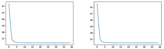
Figure 1. Empirical squared distance without IS during training (left) and on the validation data (right).

Figure 2 shows the empirical evaluation of (a) and (b) of Section 3.2 on the test data after each training epoch.

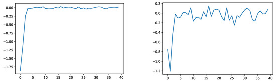
Figure 2. Empirical evaluation of (a) (left) and (b) (right) of Section 3.2.

Similarly, Figure 3 illustrates the empirical evaluation of (c) of Section 3.2 on the test data after each training epoch for the sets

$$B_1=\left\{x\in \mathbb{R}:x<s_{40\%}\right\}\mathrm{and}{B}_2=\left\{x\in \mathbb{R}:x>s_{70\%}\right\},$$

where $s_{\beta }$ denotes the $\beta$-quantile of $X=S_{\tau }$.

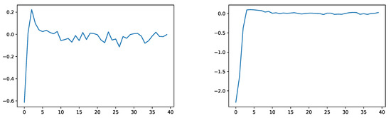
Figure 3. Empirical evaluation of (c) of Section 3.2 for the sets $B_1$ (left) and $B_2$ (right).

Training, validation and testing with IS worked similarly.

Once the network has been trained and tested, one can estimate VaR and ES numbers. Figure 4 shows our results for increasing sample sizes. The left panel shows our estimate of ${\mathrm{VaR}}_{99.5\%}\left(L\right)$ without and with IS. Plugging the 0.5%-quantile of $S_{\tau }$ into the Black–Scholes formula gives a reference value of 8.3356. Our method yielded 8.3358 without and 8.3424 with importance sampling. The right panel shows our results for ${\mathrm{ES}}_{99\%}\left(L\right)$. Transforming simulations of $S_{\tau }$ with the Black–Scholes formula and using the empirical ES estimate (5) resulted in a reference value of 8.509. Without importance sampling, the neural network learned a value of 8.456 versus 8.478 with importance sampling. It can be seen that in both cases, IS made the method more efficient. It has to be noted that for increasing sample sizes, the VaR and ES estimates converge to the corresponding risk figures in the neural network model, which are not exactly equal to their analogs in the correct model. But it can be seen that the blue lines are close to their final values after very few simulations.

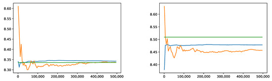
Figure 4. Convergence of the empirical 99.5%-VaR (left) and 99%-ES (right) without IS (orange) and with IS (blue) compared to the reference values obtained from the Black–Scholes formula (green).

4.2. Portfolio of Call and Put Options

In our second example we introduce a larger set of risk factors. We consider a portfolio of 20 short call and put options on different underlying assets with initial prices $s_0^i>0$ and dynamics

$$d{S}_t^i={\mu }_i{S}_t^{i}dt+{\sigma }_i{S}_t^{i}d{W}_t^{\mathbb{P},i}=r{S}_t^{i}dt+{\sigma }_i{S}_t^{i}d{W}_t^{\mathbb{Q},i}$$

for $\mathbb{P}$-Brownian motions $W^{\mathbb{P},i}$ and $\mathbb{Q}$-Brownian motions $W^{\mathbb{Q},i}$, $i=1,\cdots ,20$ such that $(W^{\mathbb{P},1},\cdots ,W^{\mathbb{P},20})$ is a multivariate Gaussian process under $\mathbb{P}$ with an instantaneous correlation of 30% between different components and $(W^{\mathbb{Q},1},\cdots ,W^{\mathbb{Q},20})$ is a multivariate Gaussian process under $\mathbb{Q}$, also with instantaneous correlation of 30% between different components. We set $s_0^i=100$ for all $i=1,\cdots ,20$ and $r=1\%$. The drift and volatility parameters are assumed to be ${\mu }_i={\mu }_{10+i}=(3+i/2)\%$ and ${\sigma }_i={\sigma }_{10+i}=(15+i)\%$, $i=1,\dots ,10$. As in the first example, we choose a maturity of $T=1/3$ and a risk horizon of $\tau =1/52$. We assume all options have the same strike price $K=100$. Then the time-$\tau$ value of the liability is

$$L=e^{-r(T-\tau )}\mathbb{E}\left[\sum _{i=1}^{10}{(S_T^i-K)}^{+}+\sum _{i=11}^{20}{(K-S_T^i)}^{+}|X\right],$$

where X is the vector $\left(S_{\tau }^1,\dots ,S_{\tau }^{20}\right)$.

In this example we trained a neural network with two hidden layers containing 15 nodes each. We first simulated according to $\mathbb{P}\otimes \mathbb{Q}$ and trained for 100 epochs. Figure 5 shows the decay of the empirical squared distance on the training and validation data set.

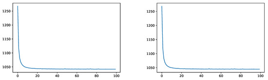
Figure 5. Empirical squared distance without IS during training (left) and on the validation data (right).

After training and testing the network under $\mathbb{P}\otimes \mathbb{Q}$, we did the same under ${\mathbb{P}}^{\nu }\otimes \mathbb{Q}$ for the IS distributions $\nu$ resulting from the procedure of Section 2.4 for $\alpha =99.5\%$ (for VaR) and $99\%$ (for ES). The two plots in Figure 6 show the empirical evaluations of (a) and (b) on the test data under the IS measure ${\mathbb{P}}^{\nu }\otimes \mathbb{Q}$ corresponding to $\alpha =99\%$.

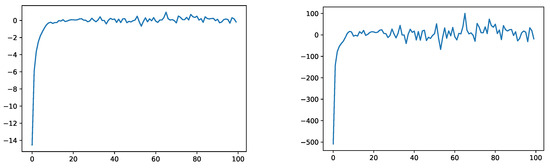
Figure 6. Empirical evaluation of (a) (left) and (b) (right) of Section 3.2 under ${\mathbb{P}}^{\nu }\otimes \mathbb{Q}$ corresponding to $\alpha =99\%$.

As an additional test, we consider the two sets

$$B_1=\{x\in {\mathbb{R}}^{20}:x_i>s_{20\%}^i \mathrm{and} x_{10+i}<s_{80\%}^{10+i} \mathrm{for} i=1,2,3\}$$

and

$$B_2=\{x\in {\mathbb{R}}^{20}:x_i<s_{80\%}^i \mathrm{and} x_{10+i}>s_{20\%}^{10+i} \mathrm{for} i=1,2,3\},$$

where $s_{\beta }^i$ is the $\beta$-quantile of $S_{\tau }^i$ under ${\mathbb{P}}^{\nu }\otimes \mathbb{Q}$, and evaluate (c) on the test data generated under the IS distribution ${\mathbb{P}}^{\nu }\otimes \mathbb{Q}$ corresponding to $\alpha =99\%$. The results are depicted in Figure 7.

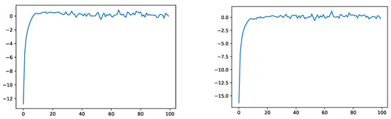
Figure 7. Empirical evaluation of (c) of Section 3.2 for the sets $B_1$ (left) and $B_2$ (right) under ${\mathbb{P}}^{\nu }\otimes \mathbb{Q}$ corresponding to $\alpha =99\%$.

After training and testing, we generated simulations of X to estimate ${\mathrm{VaR}}_{99.5\%}\left(L\right)$ and ${\mathrm{ES}}_{99\%}\left(L\right)$. The convergence for increasing sample sizes is shown in Figure 8. The reference values, 104.92 for $99.5\%$-VaR and 105.59 for $99\%$-ES, were obtained from the empirical estimates (5) by simulating $S_{\tau }$ and using the Black–Scholes formula for each of the 20 options. The neural network estimates of $99.5\%$-VaR were 104.56 without and 104.48 with IS. Those of $99\%$-ES were 105.03 without and 104.65 with IS. In both cases, IS made the procedure more efficient.

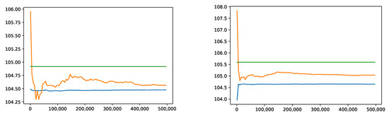
Figure 8. Convergence of the empirical 99.5%-VaR (left) and 99%-ES (right) without IS (orange) and with IS (blue) compared to the reference values obtained from the Black–Scholes formula (green).

4.3. Variable Annuity with GMIB

As a third example we study a variable annuity (VA) with guaranteed minimum income benefit (GMIB). We consider the contract analyzed by Ha and Bauer (2019) using polynomial regression. At time 0 the contract is sold to an x-year old policyholder. If she is still alive at maturity T, she can choose between the balance of an underlying investment account and a lifetime annuity. Therefore, in case of survival, the time-T value of the contract is

$$max\left\{S_T,b{a}_{x+T}\left(T\right)\right\},$$

where $S_T$ is the account value, b a guaranteed rate and $a_{x+T}\left(T\right)$ the time-T value of an annuity paying one unit of currency to a $(x+T)$-year old policyholder at times $T+1,T+2,...$ for as long as the person lives.

The contract is exposed to three types of risk: investment risk, interest rate risk and mortality risk. We suppose the log-account value $q_t=log\left(S_t\right)$, the interest rate $r_t$ and the mortality rate ${\mu }_{x+t}$ of our policyholder start from known constants $q_0,r_0,{\mu }_x$ and for $x+t\le 120$, have $\mathbb{P}$-dynamics

$$\begin{array}{cc}\hfill d{q}_t& =\left(m-\frac{1}{2}{\sigma }_S^2\right)dt+{\sigma }_{S}d{W}_t^{\mathbb{P},S},\hfill \\ \hfill d{r}_t& =\zeta (\gamma -r_t)dt+{\sigma }_{r}d{W}_t^{\mathbb{P},r},\hfill \\ \hfill d{\mu }_{x+t}& =\kappa {\mu }_{x+t}dt+{\sigma }_{\mu }d{W}_t^{\mathbb{P},\mu },\hfill \end{array}$$

for given parameters $m,\zeta ,\gamma ,\kappa ,{\sigma }_S,{\sigma }_r,{\sigma }_{\mu }$ and $\mathbb{P}$-Brownian motions $W^{\mathbb{P},S},$ $W^{\mathbb{P},r}$ and $W^{\mathbb{P},\mu }$ forming a three-dimensional Gaussian process with instantaneous correlations ${\rho }_{12}$, ${\rho }_{13}$ and ${\rho }_{23}$. We assume that our policyholder does not live longer than 120 years. Therefore, we set ${\mu }_{x+t}\equiv \infty$ for $x+t>120$. The dynamics for $x+t\le 120$ under the risk-neutral probability $\mathbb{Q}$ are assumed to be

$$\begin{array}{cc}\hfill d{q}_t& =\left(r_t-\frac{1}{2}{\sigma }_S^2\right)dt+{\sigma }_{S}d{W}_t^{\mathbb{Q},S},\hfill \\ \hfill d{r}_t& =\zeta (\overline{\gamma }-r_t)dt+{\sigma }_{r}d{W}_t^{\mathbb{Q},r},\hfill \\ \hfill d{\mu }_{x+t}& =\kappa {\mu }_{x+t}dt+{\sigma }_{\mu }d{W}_t^{\mathbb{Q},\mu },\hfill \end{array}$$

where $W^{\mathbb{Q},S},$ $W^{\mathbb{Q},r},$ $W^{\mathbb{Q},\mu }$ are $\mathbb{Q}$-Brownian motions constituting a three-dimensional Gaussian process with the same instantaneous correlations as the corresponding $\mathbb{P}$-Brownian motions. As Ha and Bauer (2019), we assume there is no risk premium for mortality and a constant risk premium $\lambda$ for interest rate risk, such that $\overline{\gamma }=\gamma -\lambda {\sigma }_r/\zeta .$ Provided that the policyholder is still alive at the risk horizon $\tau <T$, the value of the contract at that time is

$$L={\mathbb{E}}^{\mathbb{Q}}\left[e^{-{\int }_{\tau }^T{r}_s+{\mu }_{x+s}ds}max\left\{e^{q_T},b{a}_{x+T}\left(T\right)\right\}\mid X\right],$$

where we denote $X=(q_{\tau },r_{\tau },{\mu }_{x+\tau })$. Discounting with $r_s+{\mu }_{x+s}$ takes into account that the policyholder might die between $\tau$ and T. On the other hand, a possible death time between 0 and $\tau$ is not considered. This results in a conservative estimate of the capital requirement for the issuer of the contract. Alternatively, one could model the loss as $I_{A}L$, where $A\subseteq \mathsf{\Omega }$ is the event that the policyholder survives until time $\tau$.

We follow Ha and Bauer (2019) and set $x=55$, $\tau =1$, $T=15$, $b=10.792$, $q_0=4.605$, $m=5\%$, ${\sigma }_S=18\%$, $r_0=2.5\%$, $\zeta =25\%$, $\gamma =2\%$, ${\sigma }_r=1\%$, $\lambda =2\%$, ${\mu }_x=1\%$, $\kappa =7\%$, ${\sigma }_{\mu }=0.12\%$, ${\rho }_{12}=-30\%$, ${\rho }_{13}=6\%$, ${\rho }_{23}=-4\%$. Then

$$a_{x+T}\left(T\right)=\sum _{k=1}^{50}{}_k{E}_{x+T}\left(T\right),$$

where

$${}_k{E}_{x+t}\left(t\right)={\mathbb{E}}^{\mathbb{Q}}\left[e^{-{\int }_t^{t+k}{r}_s+{\mu }_{x+s}ds}\mid r_t,{\mu }_{x+t}\right]$$

is the time-t value of a pure endowment contract with maturity $t+k$. Since r and $\mu$ are affine, one has

$${}_k{E}_{x+t}\left(t\right)=F(t,k,r_t,{\mu }_{x+t})$$

for the function $F(t,k,r_t,{\mu }_{x+t})=A(t,t+k)e^{-B_r(t,t+k)r_t-B_{\mu }(t,t+k){\mu }_{x+t}}$, with $A,B_r,$ and $B_{\mu }$ as given in the Appendix of Ha and Bauer (2019). Moreover, one can write

$$L={}_{T-\tau }{E}_{x+\tau }\left(\tau \right){\mathbb{E}}^{{\mathbb{Q}}_E}\left[max\left\{e^{q_T},b{a}_{x+T}\left(T\right)\right\}\mid X\right]$$

for the probability measure ${\mathbb{Q}}_E$ given by

$$\frac{d{\mathbb{Q}}_E}{d\mathbb{Q}}=\frac{exp\left(-{\int }_0^T{r}_s+{\mu }_{x+s}ds\right)}{{\mathbb{E}}^{\mathbb{Q}}exp\left(-{\int }_0^T{r}_s+{\mu }_{x+s}ds\right)}.$$

Under $\mathbb{P}$, $X=(q_{\tau },r_{\tau },{\mu }_{\tau })$ is a three-dimensional normal vector, and the conditional ${\mathbb{Q}}_E$-distribution of $(q_T,r_T,{\mu }_{x+T})$ given X is normal too (the precise form of these distributions is given in the Appendix of Ha and Bauer (2019)). This makes it possible to efficiently simulate $(X,Y)$ under $\mathbb{P}\otimes {\mathbb{Q}}_E$, where

$$Y=F(\tau ,T-\tau ,r_{\tau },{\mu }_{x+\tau })max\left\{e^{q_T},b\sum _{k=1}^{50}F(T,k,r_T,{\mu }_{x+T})\right\}.$$

To approximate L we chose a network with two hidden layers containing 4 nodes each and trained it for 40 epochs. Figure 9 shows the empirical squared distance without IS on the training and validation data set.

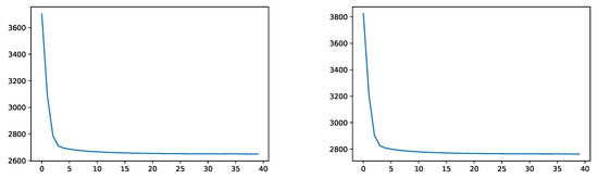
Figure 9. Empirical squared distance without IS during training (left) and on the validation data (right).

The panels in Figure 10 illustrate the empirical evaluations of the test criteria (a) and (b) from Section 3.2.

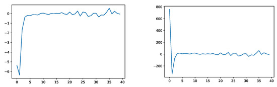
Figure 10. Empirical evaluation of (a) (left) and (b) (right) of Section 3.2 under $\mathbb{P}\otimes {\mathbb{Q}}_E$.

To test (c) from Section 3.2 we considered the sets

$$B_1=\left\{x\in {\mathbb{R}}^3:x_1>q_{70\%} \mathrm{and} x_2<r_{30\%}\right\}\mathrm{and}{B}_2=\left\{x\in {\mathbb{R}}^3:x_1<q_{30\%} \mathrm{and} x_2>r_{70\%}\right\}$$

where $q_{\beta }$ and $r_{\beta }$ denote the $\beta$-quantiles of $q_{\tau }$ and $r_{\tau }$ under $\mathbb{P}\otimes {\mathbb{Q}}_E$; see Figure 11.

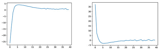
Figure 11. Empirical evaluation of (c) of Section 3.2 for the sets $B_1$ (left) and $B_2$ (right) under $\mathbb{P}\otimes {\mathbb{Q}}_E$.

We also trained and tested under ${\mathbb{P}}^{\nu }\otimes {\mathbb{Q}}_E$ for an IS distribution $\nu$ on ${\mathbb{R}}^d$. Our results are reported in Figure 12. Our estimate of ${\mathrm{VaR}}_{99.5\%}\left(L\right)$ was 138.64 without and 138.52 with IS. In comparison, the VaR estimate obtained by Ha and Bauer (2019) using 37 monomials and 40 million simulations is 139.74. Our estimates of ${\mathrm{ES}}_{99\%}\left(L\right)$ came out as 141.12 without and 142.12 with IS. There exist no reference values for this case.

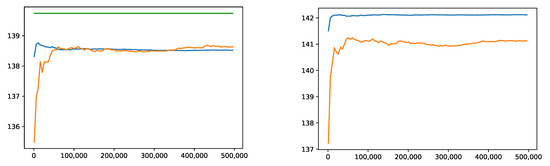
Figure 12. Convergence of the empirical 99.5%-VaR (left) and 99%-ES (right) without IS (orange) and with IS (blue) compared to the reference value from Ha and Bauer (2019) (green).

5. Conclusions

In this paper we have developed a deep learning method for assessing the risk of an asset-liability portfolio over a given time horizon. It first computes a neural network approximation of the portfolio value at the risk horizon. Then the approximation is used to estimate a risk measure, such as value-at-risk or expected shortfall, from Monte Carlo simulations. We have investigated how to choose the architecture of the network, how to learn the network parameters under a suitable importance sampling distribution and how to test the adequacy of the network approximation. We have illustrated the approach by computing value-at-risk and expected shortfall in three typical risk assessment problems from banking and insurance. In all cases the approach has worked efficiently and produced accurate results.

References

- Bauer, Daniel, Andreas Reuss, and Daniela Singer. 2012. On the calculation of the solvency capital requirement based on nested simulations. ASTIN Bulletin 42: 453–99. [Google Scholar]
- Britten-Jones, Mark, and Stephen Schaefer. 1999. Non-linear Value-at-Risk. Review of Finance, European Finance Association 5: 155–80. [Google Scholar]
- Broadie, Mark, Yiping Du, and Ciamac Moallemi. 2011. Efficient risk estimation via nested sequential estimation. Management Science 57: 1171–94. [Google Scholar] [CrossRef]
- Broadie, Mark, Yiping Du, and Ciamac Moallemi. 2015. Risk estimation via regression. Operations Research 63: 1077–97. [Google Scholar] [CrossRef]
- Bru, Bernard, and Henri Heinich. 1985. Meilleures approximations et médianes conditionnelles. Annales de l’I.H.P. Probabilités et Statistiques 21: 197–224. [Google Scholar]
- Cambou, Mathieu, and Damir Filipović. 2018. Replicating portfolio approach to capital calculation. Finance and Stochastics 22: 181–203. [Google Scholar] [CrossRef]
- Carriere, Jacques F. 1996. Valuation of the early-exercise price for options using simulations and nonparametric regression. Insurance: Mathematics and Economics 19: 19–30. [Google Scholar] [CrossRef]
- Castellani, Gilberto, Ugo Fiore, Zelda Marino, Luca Passalacqua, Francesca Perla, Salvatore Scognamiglio, and Paolo Zanetti. 2019. An Investigation of Machine Learning Approaches in the Solvency II Valuation Framework. SSRN Preprint. [Google Scholar]
- Cybenko, G. 1989. Approximation by superpositions of a sigmoidal function. Mathematics of Control, Signals and Systems 2: 303–14. [Google Scholar] [CrossRef]
- David, Herbert A., and Haikady N. Nagaraja. 2003. Order Statistics, 3rd ed. Wiley Series in Probability and Statistics; Hoboken: Wiley. [Google Scholar]
- Duffie, Darrell, and Jun Pan. 2001. Analytical Value-at-Risk with jumps and credit risk. Finance and Stochastics 5: 155–80. [Google Scholar] [CrossRef]
- Fiore, Ugo, Zelda Marino, Luca Passalacqua, Francesca Perla, Salvatore Scognamiglio, and Paolo Zanetti. 2018. Tuning a deep learning network for Solvency II: Preliminary results. In Mathematical and Statistical Methods for Actuarial Sciences and Finance: MAF 2018. Berlin: Springer. [Google Scholar]
- Glasserman, Paul. 2003. Monte Carlo Methods in Financial Engineering. Stochastic Modelling and Applied Probability. Berlin: Springer. [Google Scholar]
- Glorot, Xavier, and Yoshua Bengio. 2010. Understanding the difficulty of training deep feedforward neural networks. Proceedings of the Thirteenth International Conference on Artificial Intelligence and Statistics 9: 249–56. [Google Scholar]
- Glynn, Peter, and Shing-Hoi Lee. 2003. Computing the distribution function of a conditional expectation via Monte Carlo: Discrete conditioning spaces. ACM Transactions on Modeling and Computer Simulation 13: 238–58. [Google Scholar]
- Goodfellow, Ian, Yoshua Bengio, and Aaron Courville. 2016. Deep Learning. Cambridge: MIT Press. [Google Scholar]
- Gordy, Michael B., and Sandeep Juneja. 2008. Nested simulation in portfolio risk measurement. Management Science 56: 1833–48. [Google Scholar] [CrossRef]
- Ha, Hongjun, and Daniel Bauer. 2019. A least-squares Monte Carlo approach to the estimation of enterprise risk. Working Paper. Forthcoming. [Google Scholar]
- Hejazi, Seyed Amir, and Kenneth R. Jackson. 2017. Efficient valuation of SCR via a neural network approach. Journal of Computational and Applied Mathematics 313: 427–39. [Google Scholar] [CrossRef]
- Hornik, Kurt, Maxwell Stinchcombe, and Halbert White. 1989. Multilayer feedforward networks are universal approximators. Neural Networks 2: 359–66. [Google Scholar] [CrossRef]
- Lee, Shing-Hoi. 1998. Monte Carlo Computation of Conditional Expectation Quantiles. Ph.D. thesis, Stanford University, Stanford, CA, USA. [Google Scholar]
- Leshno, Moshe, Vladimir Lin, Allan Pinkus, and Shimon Schocken. 1993. Multilayer feedforward networks with a non-polynomial activation function can approximate any function. Neural Networks 6: 861–67. [Google Scholar] [CrossRef]
- Longstaff, Francis, and Eduardo Schwartz. 2001. Valuing American options by simulation: A simple least-squares approach. The Review of Financial Studies 14: 113–47. [Google Scholar] [CrossRef]
- McNeil, Alexander J., Rüdiger Frey, and Paul Embrechts. 2015. Quantitative Risk Management: Concepts, Techniques and Tools, rev. ed. Princeton: Princeton University Press. [Google Scholar]
- Natolski, Jan, and Ralf Werner. 2017. Mathematical analysis of replication by cashflow matching. Risks 5: 13. [Google Scholar] [CrossRef]
- Pelsser, Antoon, and Janina Schweizer. 2016. The difference between LSMC and replicating portfolio in insurance liability modeling. European Actuarial Journal 6: 441–94. [Google Scholar] [CrossRef] [PubMed]
- Rouvinez, Christophe. 1997. Going Greek with VaR. Risk Magazine 10: 57–65. [Google Scholar]
- Ruder, Sebastian. 2016. An overview of gradient descent optimization algorithms. arXiv arXiv:1609.04747. [Google Scholar]
- Tsitsiklis, John, and Benjamin Van Roy. 2001. Regression methods for pricing complex American-style options. IEEE Transactions on Neural Networks 12: 694–703. [Google Scholar] [CrossRef] [PubMed]
- Wüthrich, Mario V. 2016. Market-Consistent Actuarial Valuation. EAA Series; Berlin: Springer. [Google Scholar]
- Zwingmann, Tobias, and Hajo Holzmann. 2016. Asymptotics for the expected shortfall. arXiv arXiv:1611.07222. [Google Scholar]