An Urn-Based Nonparametric Modeling of the Dependence between PD and LGD with an Application to Mortgages


Abstract
:1. Introduction
- An intuitive bivariate model is proposed for the joint modeling of PD and LGD. The construction exploits the power of Polya urns to generate a Bayesian nonparametric approach to wrong-way risk. The model can be interpreted as a mixture model, following the typical credit risk management classification (McNeil et al. 2015).
- The proposed model is able to combine prior beliefs with empirical evidence and, exploiting the reinforcement mechanism embedded in Polya urns, it learns, thus improving its performances over time.
- The ability of learning and improving gives the model a machine/deep learning flavour. However, differently from the common machine/deep learning approaches, the behavior of the new model can be controlled and studied in a rigorous way from a probabilistic point of view. In other words, the common “black box” argument (Knight 2017) of machine/deep learning does not apply.
- The possibility of eliciting an a priori allows for the exploitation of experts’ judgements, which can be extremely useful when dealing with rare events, historical bias and data problems in general (Cheng and Cirillo 2018; Derbyshire 2017; Shackle 1955).
- The model we propose can only deal with positive dependence. Given the empirical literature, this is not a problem in WWR modeling; however, it is important to be aware of this feature, if other applications are considered.
2. Model
2.1. The Two-Color RUP
2.2. Modeling Dependence
- (1)
- Given the observations and , the sequence is generated via a Gibbs sampling. The full conditional of , , is such thatSince is exchangeable, all the other full conditionals, , where , have an analogous form.
- (2)
- Once is obtained, compute and .
- (3)
- The quantities , , and are then sampled according to their beta-Stacy predictive distributions , , and as per Equation (3).
- (4)
- Finally, set and .
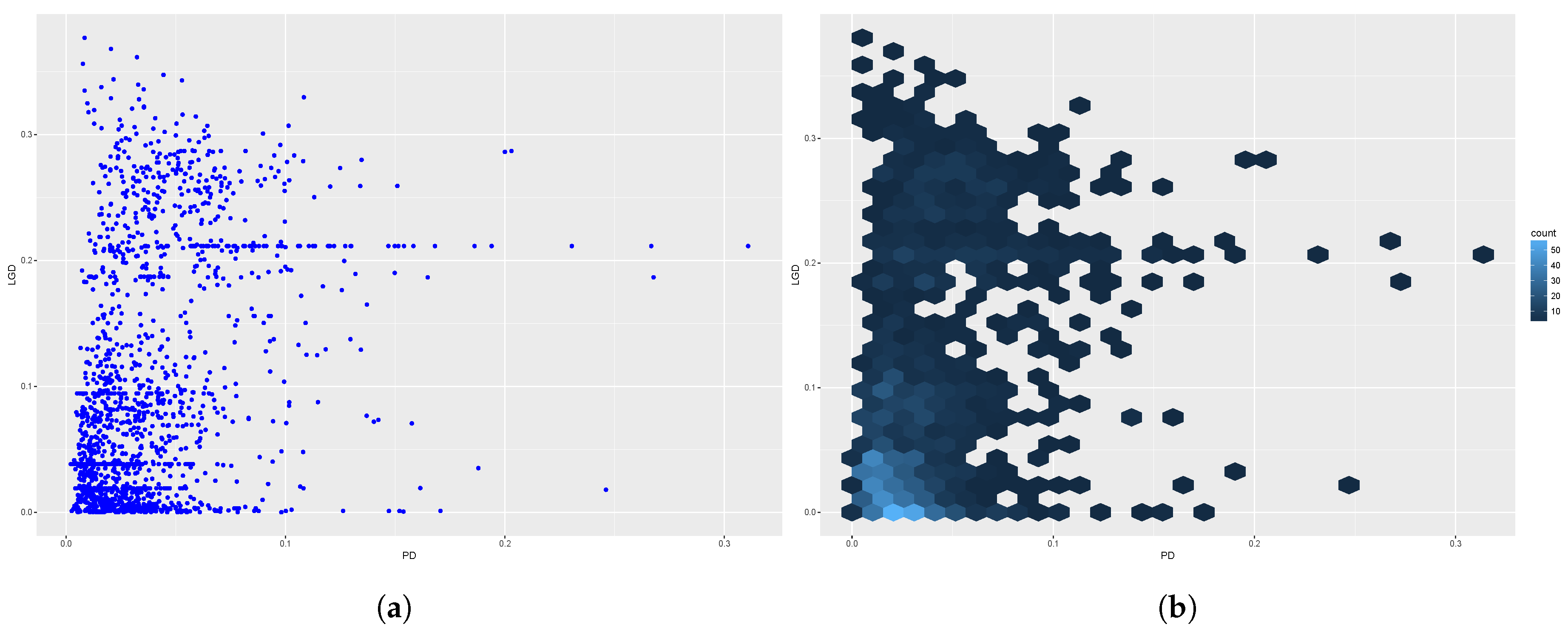
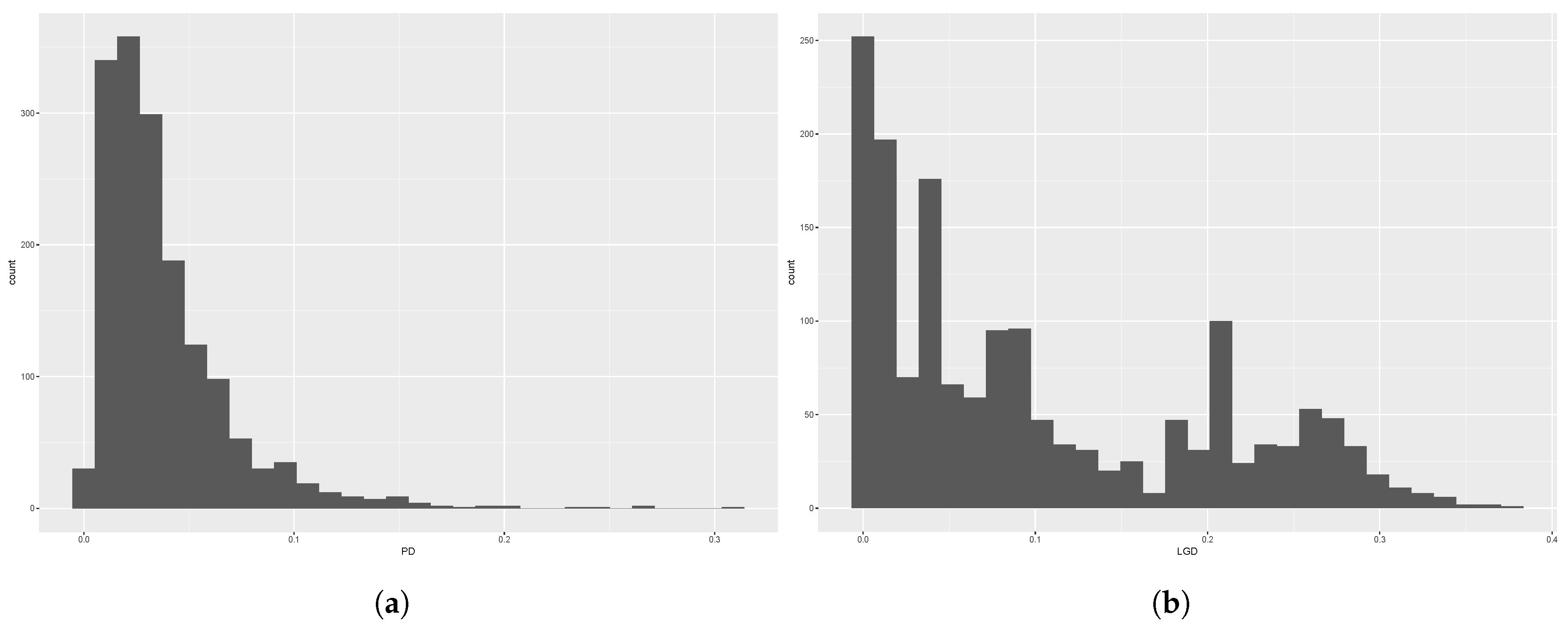
3. Data
4. Results
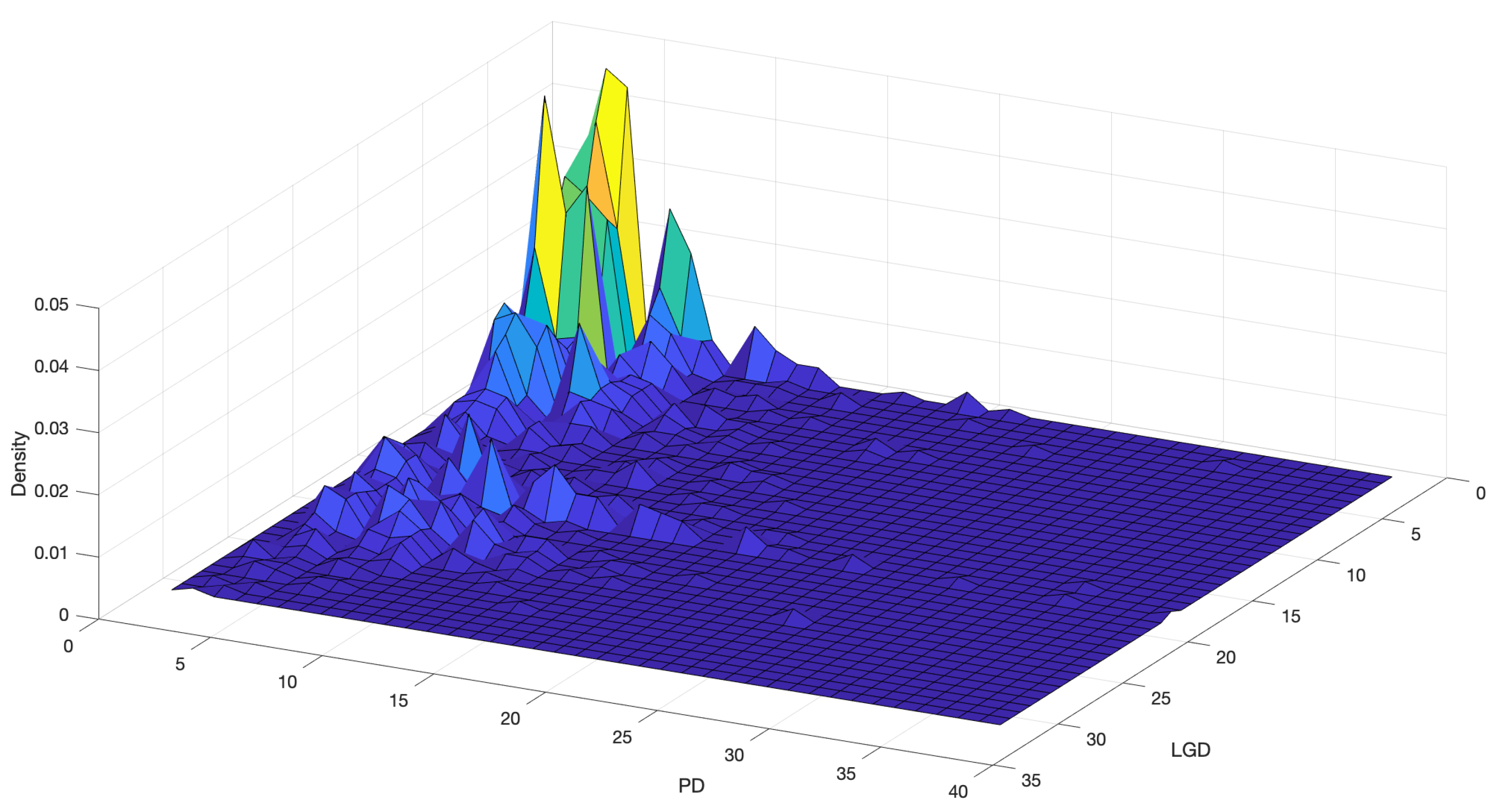
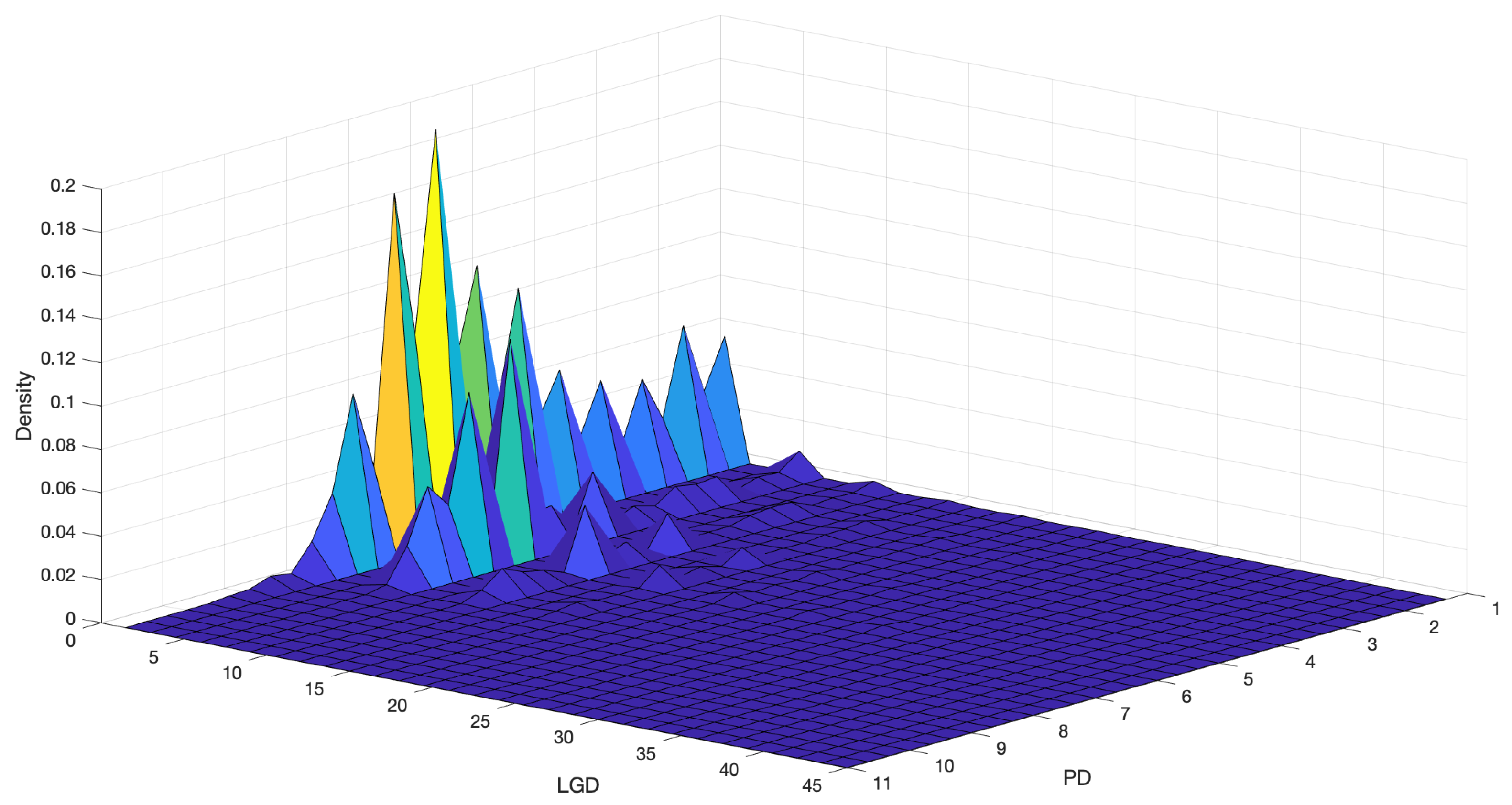
4.1. Discretisation
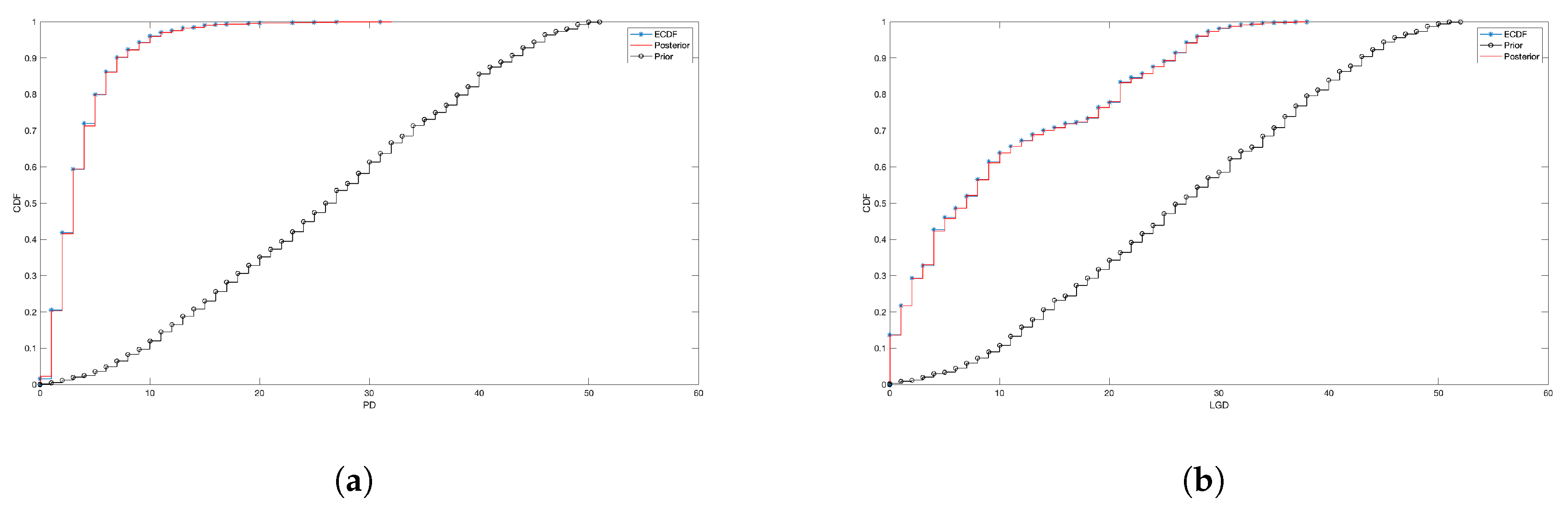
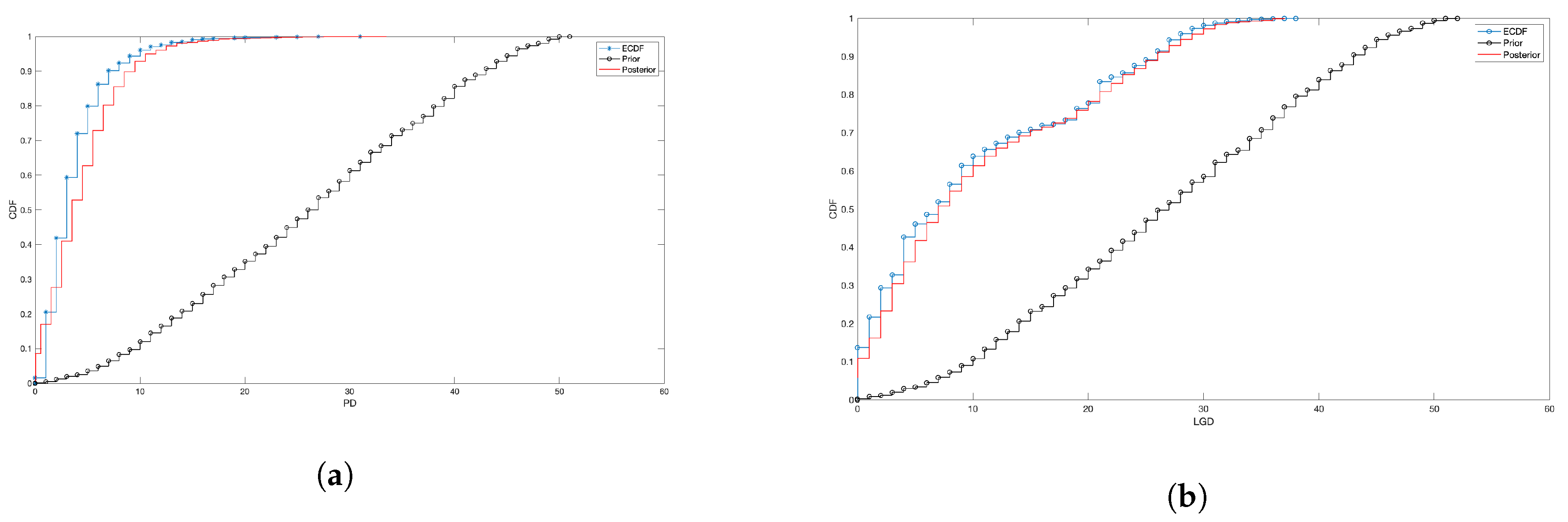
4.2. Prior Elicitation
- Independent discrete uniforms for , and , where the range of variation for B and C is simply inherited from X and Y (but extra conditions can be applied, if needed), while for A the range is chosen to guarantee . For instance, if the covariance between X and Y is approximately 3, the interval guarantees that as well. We can simply use the formula for the variance of a discrete uniform, i.e.,
- Independent Poisson distributions, such that , while for B and C one sets and , where is the empirical mean of X. This guarantees, for example, that . Recall in fact that, in a Poisson random variable, the mean and the variance are both equal to the intensity parameter, and independent Poissons are closed under convolution. Given our data, where the empirical variances of X and Y are not at all equal to the empirical means, but definitely larger, the Poisson prior can be seen as an example of a wrong prior.
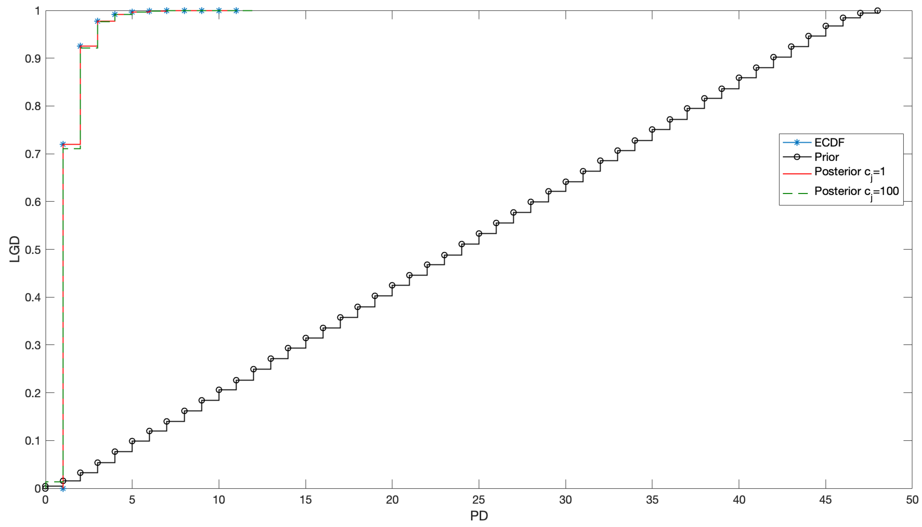
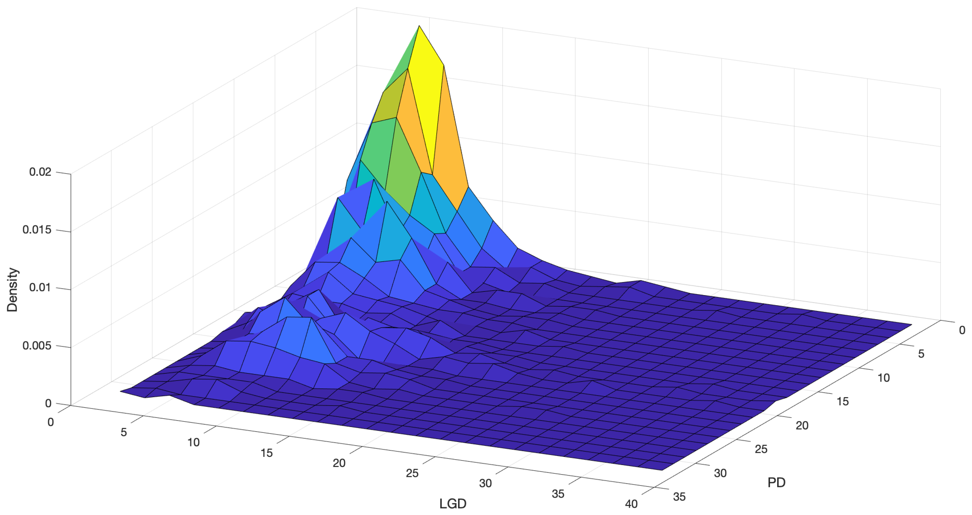
4.3. Fitting
4.4. What about the Crisis?
5. Conclusions
Author Contributions
Funding
Acknowledgments
Conflicts of Interest
References
- Altman, Edward I. 2006. Default Recovery Rates and LGD in Credit Risk Modeling and Practice: An Updated Review of the Literature and Empirical Evidence. New York University, Stern School of Business. [Google Scholar] [CrossRef]
- Altman, Edward I., Andrea Resti, and Andrea Sironi. 2001. Analyzing and Explaining Default Recovery Rates. A Report Submitted to the International Swaps & Derivatives Association. Available online: http://people.stern.nyu.edu/ealtman/Review1.pdf (accessed on 14 January 2019).
- Altman, Edward I., Brooks Brady, Andrea Resti, and Andrea Sironi. 2005. The Link between Default and Recovery Rates: Theory, Empirical Evidence, and Implications. The Journal of Business 78: 2203–27. [Google Scholar] [CrossRef]
- Amerio, Emanuele, Pietro Muliere, and Piercesare Secchi. 2004. Reinforced Urn Processes for Modeling Credit Default Distributions. International Journal of Theoretical and Applied Finance 7: 407–23. [Google Scholar] [CrossRef]
- Baesens, Bart, Daniel Roesch, and Harald Scheule. 2016. Credit Risk Analytics: Measurement Techniques, Applications, and Examples in SAS. Hoboken: Wiley. [Google Scholar]
- BCBS. 2000. Principles for the Management of Credit Risk. Available online: https://www.bis.org/publ/bcbs75.pdf (accessed on 10 March 2019).
- BCBS. 2005. An Explanatory Note on the Basel II IRB Risk Weight Functions. Available online: https://www.bis.org/bcbs/irbriskweight.pdf (accessed on 10 March 2019).
- BCBS. 2006. International Convergence of Capital Measurement and Capital Standards. Number 30 June. Basel: Bank for International Settlements, p. 285. [Google Scholar]
- BCBS. 2011. Basel III: A Global Regulatory Framework for More Resilient Banks and Banking Systems. Number 1 June. Basel: Bank for International Settlements, p. 69. [Google Scholar]
- Bruche, Max, and Carlos Gonzalez-Aguado. 2010. Recovery Rates, Default Probabilities, and the Credit Cycle. Journal of Banking & Finance 34: 754–64. [Google Scholar]
- Bulla, Paolo. 2005. Application of Reinforced Urn Processes to Survival Analysis. Ph.D. thesis, Bocconi University, Milan, Italy. [Google Scholar]
- Bulla, Paolo, Pietro Muliere, and Steven Walker. 2007. Bayesian Nonparametric Estimation of a Bivariate Survival Function. Statistica Sinica 17: 427–44. [Google Scholar]
- Calabrese, Raffaella, and Paolo Giudici. 2015. Estimating Bank Default with Generalised Extreme Value Regression Models. Journal of the Operational Research Society 28: 1–10. [Google Scholar] [CrossRef]
- Cerchiello, Paola, and Paolo Giudici. 2014. Bayesian Credit Rating Assessment. Communications in Statistics: Theory and Methods 111: 101–15. [Google Scholar]
- Cheng, Dan, and Pasquale Cirillo. 2018. A Reinforced Urn Process Modeling of Recovery Rates and Recovery Times. Journal of Banking & Finance 96: 1–17. [Google Scholar]
- Cirillo, Pasquale, Jürg Hüsler, and Pietro Muliere. 2010. A Nonparametric Urn-based Approach to Interacting Failing Systems with an Application to Credit Risk Modeling. International Journal of Theoretical and Applied Finance 41: 1–18. [Google Scholar] [CrossRef]
- Cirillo, Pasquale, Jürg Hüsler, and Pietro Muliere. 2013. Alarm Systems and Catastrophes from a Diverse Point of View. Methodology and Computing in Applied Probability 15: 821–39. [Google Scholar] [CrossRef]
- Derbyshire, James. 2017. The Siren Call of Probability: Dangers Associated with Using Probability for Consideration of the Future. Futures 88: 43–54. [Google Scholar] [CrossRef]
- Diaconis, Persi, and David Freedman. 1980. De Finetti’s Theorem for Markov Chains. The Annals of Probability 8: 115–30. [Google Scholar] [CrossRef]
- Duffie, Darrell. 1998. Defaultable Term Structure Models with Fractional Recovery of Par. Technical Report. Stanford: Graduate School of Business, Stanford University. [Google Scholar]
- Duffie, Darrell, and Kenneth J. Singleton. 1999. Modeling Term Structures of Defaultable Bonds. The Review of Financial Studies 12: 687–720. [Google Scholar] [CrossRef] [Green Version]
- Duffie, Darrell, and Kenneth J. Singleton. 2003. Credit Risk. Cambridge: Cambridge University Press. [Google Scholar]
- Eichengreen, Barry, Ashoka Mody, Milan Nedeljkovic, and Lucio Sarno. 2012. How the Subprime Crisis Went Global: Evidence from Bank Credit Default Swap Spreads. Journal of International Money and Finance 31: 1299–318. [Google Scholar] [CrossRef]
- Experian. 2019. Blog: What Are the Different Credit Scoring Ranges? Available online: https://www.experian.com/blogs/ask-experian/infographic-what-are-the-different-scoring-ranges/ (accessed on 18 January 2019).
- Figini, Silvia, and Paolo Giudici. 2011. Statistical Merging of Rating Models. Journal of the Operational Research Society 62: 1067–74. [Google Scholar] [CrossRef]
- Fortini, Sandra, and Sonia Petrone. 2012. Hierarchical Reinforced Urn Processes. Statistics & Probability Letters 82: 1521–29. [Google Scholar]
- Freddie Mac. 2019a. Single Family Loan-Level Dataset; Freddie Mac. Available online: http://www.freddiemac.com/research/datasets/sf_loanlevel_dataset.page (accessed on 3 February 2019).
- Freddie Mac. 2019b. Single Family Loan-Level Dataset General User Guide; Freddie Mac. Available online: http://www.freddiemac.com/fmac-resources/research/pdf/user_guide.pdf (accessed on 3 February 2019).
- Freddie Mac. 2019c. Single Family Loan-Level Dataset Summary Statistics; Freddie Mac. Available online: http://www.freddiemac.com/fmac-resources/research/pdf/summary_statistics.pdf (accessed on 3 February 2019).
- Frye, Jon. 2000. Depressing Recoveries. Risk 13: 108–11. [Google Scholar]
- Frye, Jon. 2005. The Effects of Systematic Credit Risk: A False Sense of Security. In Recovery Risk. Edited by Edward Altman, Andrea Resti and Andrea Sironi. London: Risk Books, pp. 187–200. [Google Scholar]
- Galavotti, Maria Carla. 2001. Subjectivism, objectivism and objectivity in bruno de finetti’s bayesianism. In Foundations of Bayesianism. Edited by David Corfield and Jon Williamson. Dordrecht: Springer, pp. 161–74. [Google Scholar]
- Genest, Christian, and Louis-Paul Rivest. 1993. Statistical inference procedures for bivariate archimedean copulas. Journal of the American Statistical Association 88: 1034–43. [Google Scholar] [CrossRef]
- Geske, Robert. 1977. The Valuation of Corporate Liabilities as Compound Options. Journal of Financial and Quantitative Analysis 12: 541–52. [Google Scholar] [CrossRef]
- Giudici, Paolo. 2001. Bayesian Data Mining, with Application to Credit Scoring and Benchmarking. Applied Stochastic Models in Business and Industry 17: 69–81. [Google Scholar] [CrossRef]
- Giudici, Paolo, Pietro Muliere, and Maura Mezzetti. 2003. Mixtures of Dirichlet Process Priors for Variable Selection in Survival Analysis. Journal of Statistical Planning and Inference 17: 867–78. [Google Scholar]
- Hamerle, Alfred, Michael Knapp, and Nicole Wildenauer. 2011. Modelling Loss Given Default: A “Point in Time”-Approach. In The Basel II Risk Parameters: Estimation, Validation, Stress Testing—With Applications to Loan Risk Management. Edited by Bernd Engelmann and Robert Rauhmeier. Berlin: Springer, pp. 137–50. [Google Scholar]
- Hjort, Nils Lid, Chris Holmes, Peter Mueller, and Stephen G. Walker. 2010. Bayesian Nonparametrics. Cambridge: Cambridge University Press. [Google Scholar]
- Hull, John C. 2015. Risk Management and Financial Institutions, 4th ed. New York: Wiley. [Google Scholar]
- Ivashina, Victoria, and David Scharfstein. 2010. Bank lending during the financial crisis of 2008. Journal of Financial Economics 97: 319–38. [Google Scholar] [CrossRef]
- Jackman, Simon. 2009. Bayesian Analysis for the Social Sciences. New York: Wiley. [Google Scholar]
- Jones, Philip, Scott P. Mason, and Eric Rosenfeld. 1984. Contingent Claims Analysis of Corporate Capital Structures: An Empirical Investigation. The Journal of Finance 39: 611–25. [Google Scholar] [CrossRef]
- JP Morgan. 1997. Creditmetrics—Technical Document. Available online: http://www.defaultrisk.com/_pdf6j4/creditmetrics_techdoc.pdf (accessed on 3 February 2019).
- Kim, In Joon, Krishna Ramaswamy, and Suresh Sundaresan. 1993. Does Default Risk in Coupons Affect the Valuation of Corporate Bonds?: A Contingent Claims Model. Financial Management 22: 117–31. [Google Scholar] [CrossRef]
- Knight, Will. 2017. The Dark Secret at the Heart of AI. Technology Review 120: 54–63. [Google Scholar]
- Lando, David. 1998. On Cox Processes and Credit Risky Securities. Review of Derivatives Research 2: 99–120. [Google Scholar] [CrossRef]
- Lindley, Dennis. 1991. Making Decisions, 2nd ed. New York: Wiley. [Google Scholar]
- Longstaff, Francis A., and Eduardo S. Schwartz. 1995. A Simple Approach to Valuing Risky Fixed and Floating Rate Debt. The Journal of Finance 50: 789–819. [Google Scholar] [CrossRef]
- Mahmoud, Hosam. 2008. Polya Urn Models. Boca Raton: CRC Press. [Google Scholar]
- Maio, Vittorio. 2017. Modelling the Dependence between PD and LGD. A New Regulatory Capital Calculation with Empirical Analysis from the US Mortgage Market. Master’s thesis, Politecnico di Milano, Milano, Italy. Available online: https://www.politesi.polimi.it/handle/10589/137281 (accessed on 10 March 2019).
- McNeil, Alexander J., and Jonathan P. Wendin. 2007. Bayesian inference for generalized linear mixed models of portfolio credit risk. Journal of Empirical Finance 14: 131–49. [Google Scholar] [CrossRef]
- McNeil, Alexander J., Ruediger Frey, and Paul Embrechts. 2015. Quantitative Risk Management. Princeton: Princeton University Press. [Google Scholar]
- Meng, Xiao-Li. 1994. Multiple-Imputation Inferences with Uncongenial Sources of Input. Statistical Science 9: 538–58. [Google Scholar] [CrossRef]
- Merton, Robert C. 1974. On the Pricing of Corporate Debt: The Risk Structure of Interest Rates. The Journal of Finance 29: 449–70. [Google Scholar]
- Miu, Peter, and Bogie Ozdemir. 2006. Basel Requirement of Downturn LGD: Modeling and Estimating PD & LGD Correlations. Journal of Credit Risk 2: 43–68. [Google Scholar]
- Muliere, Pietro, Piercesare Secchi, and Stephen G Walker. 2000. Urn Schemes and Reinforced Random Walks. Stochastic Processes and their Applications 88: 59–78. [Google Scholar] [CrossRef]
- Muliere, Pietro, Piercesare Secchi, and Stephen G Walker. 2003. Reinforced Random Processes in Continuous Time. Stochastic Processes and Their Applications 104: 117–30. [Google Scholar] [CrossRef]
- Murphy, Kevin P. 2012. Machine Learning: A Probabilistic Perspective. Cambridge: The MIT Press. [Google Scholar]
- Narain, Bhavana. 1992. Survival Analysis and the Credit Granting Decision. In Credit Scoring and Credit Control. Edited by Lyn C. Thomas, David B. Edelman and Jonathan N. Crook. Oxford: Oxford University Press, pp. 109–21. [Google Scholar]
- Nelsen, Roger B. 2006. An Introduction to Copulas. New York: Springer. [Google Scholar]
- Nielsen, Lars Tyge, Jesus Saà-Requejo, and Pedro Santa-Clara. 2001. Default Risk and Interest Rate Risk: The Term Structure of Default Spreads. Paris: INSEAD. [Google Scholar]
- Peluso, Stefano, Antonietta Mira, and Pietro Muliere. 2015. Reinforced Urn Processes for Credit Risk Models. Journal of Econometrics 184: 1–12. [Google Scholar] [CrossRef]
- Resti, Andrea, and Andrea Sironi. 2007. Risk Management and Shareholders’ Value in Banking. New York: Wiley. [Google Scholar]
- Rueschendorf, Ludger. 2009. On the distributional transform, sklar’s theorem, and the empirical copula process. Journal of Statistical Planning and Inference 139: 3921–27. [Google Scholar] [CrossRef]
- Shackle, George Lennox Sharman. 1955. Uncertainty in Economics and Other Reflections. Cambridge: Cambridge University Press. [Google Scholar]
- Taleb, Nassim Nicholas. 2007. The Black Swan: The Impact of the Highly Improbable. New York: Random House. [Google Scholar]
- Turlakov, Mihail. 2013. Wrong-way risk, credit and funding. Risk 26: 69–71. [Google Scholar]
- Vasicek, Oldrich A. 1984. Credit Valuation. Available online: http://www.ressources-actuarielles.net/EXT/ISFA/1226.nsf/0/c181fb77ee99d464c125757a00505078/$FILE/Credit_Valuation.pdf (accessed on 10 March 2019).
- Walker, Stephen, and Pietro Muliere. 1997. Beta-Stacy Processes and a Generalization of the Pólya-Urn Scheme. The Annals of Statistics 25: 1762–80. [Google Scholar] [CrossRef]
- Wilde, Tom. 1997. CreditRisk+: A Credit Risk Management Framework. Technical Report. New York: Credit Suisse First, Boston. [Google Scholar]
- Wilson, Thomas C. 1998. Portfolio credit risk. Economic Policy Review 4: 71–82. [Google Scholar] [CrossRef]
- Witzany, Jiřì. 2011. A Two Factor Model for PD and LGD Correlation. Bulletin of the Czech Econometric Society 18. [Google Scholar] [CrossRef]
- Yao, Xiao, Jonathan Crook, and Galina Andreeva. 2017. Is It Obligor or Instrument That Explains Recovery Rate: Evidence from US Corporate Bond. Journal of Financial Stability 28: 1–15. [Google Scholar] [CrossRef]
- Zhang, Jie, and Lyn C. Thomas. 2012. Comparisons of Linear Regression and Survival Analysis Using Single and Mixture Distributions Approaches in Modelling LGD. International Journal of Forecasting 28: 204–15. [Google Scholar] [CrossRef]
| 1 | In reality, as observed in Zhang and Thomas (2012), the LGD can be slightly negative or slightly above 100% because of fees and interests; however, we exclude that situation here. In terms of applications, all negative values can be set to 0, and all values above 100 can be rounded to 100. |
| 2 | Please observe that exchangeability only applies among the couples , while within each couple there is a clear dependence, so that and are not exchangeable. |
| 3 | To avoid any copyright problem with Freddie Mac, which already freely shares its data online, from Maio’s dataset (here attached), we only provide the PD and the LGD estimates, together with the unique alphanumeric identifier. In this way, merging the data sources is straightforward. |


| Class | Number of Loans | Avg. PD | Avg. LGD | |
|---|---|---|---|---|
| Very Poor | 1627 | 0.0378 | 0.1013 | 0.3370 |
| Fair | 46,720 | 0.0238 | 0.1237 | 0.4346 |
| Good | 124,824 | 0.0138 | 0.1409 | 0.3159 |
| Very good | 177,891 | 0.0083 | 0.1574 | 0.3599 |
| Exceptional | 32,403 | 0.0080 | 0.1777 | 0.1858 |
| Class | ||||||||
|---|---|---|---|---|---|---|---|---|
| Very Poor | 3.85 | 3.81 | 3.02 | 3.03 | 3.24 | 2.53 | 0.34 | 0.20 |
| Fair | 2.41 | 2.32 | 1.50 | 1.44 | 2.36 | 2.33 | 0.45 | 0.51 |
| Good | 1.43 | 0.49 | 0.83 | 0.25 | 0.71 | 0.66 | 0.34 | 0.38 |
| Very good | 0.36 | 0.32 | 0.62 | 0.64 | 0.14 | 0.16 | 0.38 | 0.42 |
| Exceptional | 0.16 | 0.18 | 0.60 | 0.54 | 0.82 | 0.83 | 0.19 | 0.18 |
| Class | ||||||
|---|---|---|---|---|---|---|
| Very Poor | 9.82 | 10.2 | 6.63 | 6.14 | 9.51 | 8.32 |
| Fair | 12.1 | 11.5 | 9.43 | 10.6 | 9.69 | 5.53 |
| Good | 13.8 | 19.8 | 14.5 | 19.2 | 5.70 | 5.26 |
| Very good | 15.6 | 18.5 | 18.7 | 18.0 | 5.27 | 5.13 |
| Exceptional | 17.8 | 17.2 | 20.4 | 19.7 | 8.00 | 4.99 |
© 2019 by the authors. Licensee MDPI, Basel, Switzerland. This article is an open access article distributed under the terms and conditions of the Creative Commons Attribution (CC BY) license (http://creativecommons.org/licenses/by/4.0/).
Share and Cite
Cheng, D.; Cirillo, P. An Urn-Based Nonparametric Modeling of the Dependence between PD and LGD with an Application to Mortgages. Risks 2019, 7, 76. https://doi.org/10.3390/risks7030076
Cheng D, Cirillo P. An Urn-Based Nonparametric Modeling of the Dependence between PD and LGD with an Application to Mortgages. Risks. 2019; 7(3):76. https://doi.org/10.3390/risks7030076
Chicago/Turabian StyleCheng, Dan, and Pasquale Cirillo. 2019. "An Urn-Based Nonparametric Modeling of the Dependence between PD and LGD with an Application to Mortgages" Risks 7, no. 3: 76. https://doi.org/10.3390/risks7030076
APA StyleCheng, D., & Cirillo, P. (2019). An Urn-Based Nonparametric Modeling of the Dependence between PD and LGD with an Application to Mortgages. Risks, 7(3), 76. https://doi.org/10.3390/risks7030076