Estimating and Forecasting Conditional Risk Measures with Extreme Value Theory: A Review


Abstract
:1. Introduction
- Volatility-EVT. This class of models proposes a two step procedure that pre-whitens the returns with a model for the volatility and then applies a model based on EVT to the tails of the estimated residuals (Bee et al. 2016; McNeil and Frey 2000).
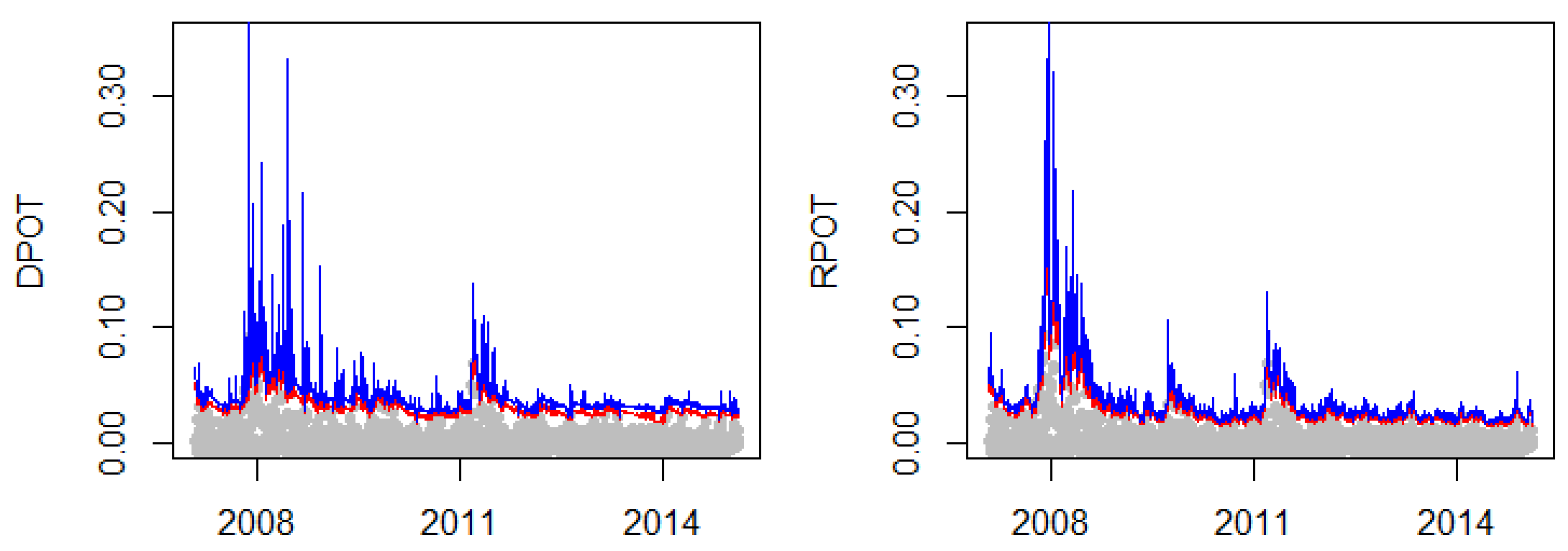
- Quantile-EVT. This class proposes using time-varying quantile models to obtain a dynamic threshold for the extremes. An extreme value model can then be applied to the exceedances over this threshold (Bee et al. 2018; Engle and Manganelli 2004).
- Time-varying EVT. This class models the returns exceeding a high constant threshold, letting the parameters of the extreme value model to be time-varying to account for the dependence in the exceedancees (Bee et al. 2015, Chavez-Demoulin et al. 2005, 2014).
2. Extreme Value Theory
2.1. Main Results
- Let with be the cumulative distribution function (cdf) of the Frechét distribution. As ,where is a slowly varying function
- Let being the cdf of the Gumbel distribution. As ,
- Let with be the cdf of the Weibull distribution. As ,where is a slowly varying function.
2.2. The Peaks over Threshold Method
3. Estimating Conditional Risk Measures with EVT
3.1. Volatility-EVT
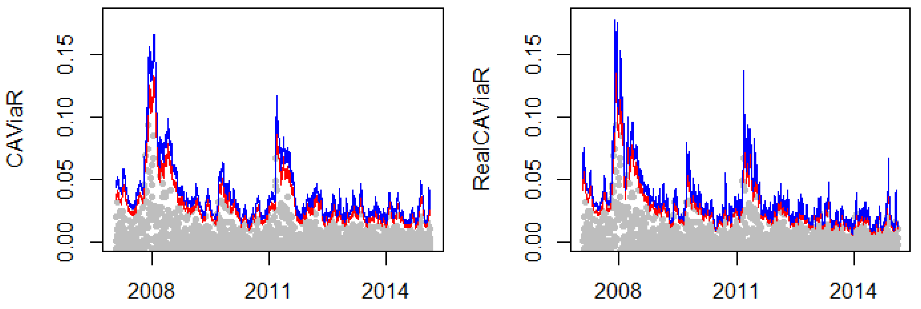
3.2. Quantile-EVT
3.3. Time-Varying EVT
4. Discussion
4.1. Volatility-EVT
4.2. Quantile-EVT
4.3. Time-Varying EVT
5. Conclusions
Author Contributions
Conflicts of Interest
References
- Artzner, Philippe, Freddy Delbaen, Jean-Marc Eber, and David Heath. 1999. Coherent measures of risk. Mathematical Finance 9: 203–28. [Google Scholar] [CrossRef]
- Basel Committee on Banking Supervision. 2013. Fundamental Review of the Trading Book: A Revised Market Risk Framework. Bank for International Settlemen. Available online: https://www.bis.org/publ/bcbs265.pdf (accessed on 13 April 2018).
- Basrak, Bojan, Richard A. Davis, and Thomas Mikosch. 2002. Regular variation of GARCH processes. Stochastic Processes and Their Applications 99: 95–115. [Google Scholar] [CrossRef]
- Bee, Marco, Dupuis Debbie Janice, and Luca Trapin. 2015. The Realized Peaks over Threshold: A High-Frequency Based Extreme Value Approach for Financial Time Series. Cahiers du Gerad G-2015-104. Montreal: GERAD. [Google Scholar]
- Bee, Marco, Debbie J. Dupuis, and Luca Trapin. 2016. Realizing the extremes: Estimation of tail-risk measures from a high-frequency perspective. Journal of Empirical Finance 36: 86–99. [Google Scholar] [CrossRef]
- Bee, Marco, Debbie J. Dupuis, and Luca Trapin. 2018. Realized extreme quantile: A joint model for conditional quantiles and measures of volatility with evt refinements. Journal of Applied Econometrics 33: 398–415. [Google Scholar] [CrossRef]
- Bollerslev, Tim. 1986. Generalized autoregressive conditional heteroskedasticity. Journal of Econometrics 31: 307–27. [Google Scholar] [CrossRef]
- Bollerslev, Tim, and Jeffrey M. Wooldridge. 1992. Quasi-maximum likelihood estimation and inference in dynamic models with time-varying covariances. Econometric Reviews 11: 143–72. [Google Scholar] [CrossRef]
- Breidt, F. Jay, and Richard A. Davis. 1998. Extremes of stochastic volatility models. Annals of Applied Probability 8: 664–75. [Google Scholar] [CrossRef]
- Brodin, Erik, and Claudia Klüppelberg. 2008. Extreme Value Theory in Finance. Hoboken: John Wiley & Sons, Ltd. [Google Scholar]
- Chavez-Demoulin, Valerie, and J. A. McGill. 2012. High-frequency financial data modeling using Hawkes processes. Journal of Banking & Finance 36: 3415–26. [Google Scholar]
- Chavez-Demoulin, Valerie, Anthony C. Davison, and Alexander J. McNeil. 2005. Estimating value-at-risk: A point process approach. Quantitative Finance 5: 227–34. [Google Scholar] [CrossRef]
- Chavez-Demoulin, Valerie, Paul Embrechts, and Sylvain Sardy. 2014. Extreme-quantile tracking for financial time series. Journal of Econometrics 181: 44–52. [Google Scholar] [CrossRef]
- Christoffersen, Peter F. 1998. Evaluating interval forecasts. International Economic Review 32: 841–62. [Google Scholar] [CrossRef]
- Cont, Rama. 2001. Empirical properties of asset returns: Stylized facts and statistical issues. Quantitative Finance 1: 223–36. [Google Scholar] [CrossRef]
- Corsi, Fulvio. 2009. A simple approximate long-memory model of realized volatility. Journal of Financial Econometrics 7: 174–96. [Google Scholar] [CrossRef]
- Creal, Drew, Siem Jan Koopman, and Andre Lucas. 2013. Generalized autoregressive score models with applications. Journal of Applied Econometrics 28: 777–95. [Google Scholar] [CrossRef]
- Davis, Richard A., and Thomas Mikosch. 2009. The extremogram: A correlogram for extreme events. Bernoulli 15: 977–1009. [Google Scholar] [CrossRef]
- Davison, Anthony C., and Richard L. Smith. 1990. Models for exceedances over high thresholds. Journal of the Royal Statistical Society. Series B 52: 393–442. [Google Scholar]
- Diebold, Francis X., Til Schuermann, and John D. Stroughair. 2000. Pitfalls and opportunities in the use of extreme value theory in risk management. The Journal of Risk Finance 1: 30–35. [Google Scholar] [CrossRef]
- Dupuis, Debbie J. 1999. Exceedances over high thresholds: A guide to threshold selection. Extremes 1: 251–61. [Google Scholar] [CrossRef]
- Embrechts, Paul, Claudia Klüppelberg, and Thomas Mikosch. 1997. Modelling Extremal Events: For Insurance and Finance. New York: Springer Science & Business Media, vol. 33. [Google Scholar]
- Engle, Robert F., and Giampiero M. Gallo. 2006. A multiple indicators model for volatility using intra-daily data. Journal of Econometrics 131: 3–27. [Google Scholar] [CrossRef]
- Engle, Robert F., and Simone Manganelli. 2004. Caviar: Conditional autoregressive value at risk by regression quantiles. Journal of Business & Economic Statistics 22: 367–81. [Google Scholar]
- Ferro, Christopher AT, and Johan Segers. 2003. Inference for clusters of extreme values. Journal of the Royal Statistical Society: Series B 65: 545–56. [Google Scholar] [CrossRef]
- Fisher, Ronald Aylmer, and Leonard Henry Caleb Tippett. 1928. Limiting forms of the frequency distribution of the largest or smallest member of a sample. In Mathematical Proceedings of the Cambridge Philosophical Society. Cambridge: Cambridge University Press, vol. 24, pp. 180–90. [Google Scholar]
- Glosten, Lawrence R., Ravi Jagannathan, and David E. Runkle. 1993. On the relation between the expected value and the volatility of the nominal excess return on stocks. The Journal of Finance 48: 1779–801. [Google Scholar] [CrossRef]
- Hansen, Bruce E. 1994. Autoregressive conditional density estimation. International Economic Review 35: 705–30. [Google Scholar] [CrossRef]
- Hansen, Peter Reinhard, Zhuo Huang, and Howard Howan Shek. 2012. Realized GARCH: A joint model for returns and realized measures of volatility. Journal of Applied Econometrics 27: 877–906. [Google Scholar] [CrossRef]
- Harvey, Campbell R., and Akhtar Siddique. 1999. Autoregressive conditional skewness. Journal of Financial and Quantitative Analysis 34: 465–87. [Google Scholar] [CrossRef]
- Heber, Gerd, Asger Lunde, Neil Shephard, and Kevin Sheppard. 2009. Oxford-Man Institute Realized Library, Version 0.2; Available online: https://realized.oxford-man.ox.ac.uk/ (accessed on 10 March 2018).
- Herrera, Rodrigo, and Adam Clements. 2018. Point process models for extreme returns: Harnessing implied volatility. Journal of Banking & Finance 88: 161–75. [Google Scholar]
- Herrera, Rodrigo, and Bernhard Schipp. 2009. Self-exciting extreme value models for stock market crashes. In Statistical Inference, Econometric Analysis and Matrix Algebra. New York: Springer, pp. 209–31. [Google Scholar]
- Herrera, Rodrigo, and Bernhard Schipp. 2013. Value at risk forecasts by extreme value models in a conditional duration framework. Journal of Empirical Finance 23: 33–47. [Google Scholar] [CrossRef]
- Jondeau, Eric, Ser-Huang Poon, and Michael Rockinger. 2007. Financial Modeling under Non-Gaussian Distributions. New York: Springer Science & Business Media. [Google Scholar]
- Koenker, Roger, and Gilbert Bassett. 1978. Regression quantiles. Econometrica 46: 33–50. [Google Scholar] [CrossRef]
- Komunjer, Ivana. 2005. Quasi-maximum likelihood estimation for conditional quantiles. Journal of Econometrics 128: 137–64. [Google Scholar] [CrossRef]
- Kuester, Keith, Stefan Mittnik, and Marc S. Paolella. 2006. Value-at-risk prediction: A comparison of alternative strategies. Journal of Financial Econometrics 4: 53–89. [Google Scholar] [CrossRef]
- Lauridsen, Sarah. 2000. Estimation of value at risk by extreme value methods. Extremes 3: 107–44. [Google Scholar] [CrossRef]
- Laurini, Fabrizio, and Jonathan A. Tawn. 2008. Regular variation and extremal dependence of garch residuals with application to market risk measures. Econometric Reviews 28: 146–69. [Google Scholar] [CrossRef]
- Li, Deyuan, and Huixia Judy Wang. 2017. Extreme quantile estimation for autoregressive models. Journal of Business & Economic Statistics. In Press. [Google Scholar]
- Simone Manganelli, Robert F. Engle. 2004. A Comparison of Value at Risk Models in Finance. Chichester: Wiley. [Google Scholar]
- Massacci, Daniele. 2016. Tail risk dynamics in stock returns: Links to the macroeconomy and global markets connectedness. Management Science 63: 3072–89. [Google Scholar] [CrossRef]
- McAleer, Michael, and Marcelo C. Medeiros. 2008. Realized volatility: A review. Econometric Reviews 27: 10–45. [Google Scholar] [CrossRef]
- McNeil, Alexander J., and Rüdiger Frey. 2000. Estimation of tail-related risk measures for heteroscedastic financial time series: An extreme value approach. Journal of Empirical Finance 7: 271–300. [Google Scholar] [CrossRef]
- Nieto, Maria Rosa, and Esther Ruiz. 2016. Frontiers in var forecasting and backtesting. International Journal of Forecasting 32: 475–501. [Google Scholar] [CrossRef]
- Patton, Andrew J., and Kevin Sheppard. 2015. Good volatility, bad volatility: Signed jumps and the persistence of volatility. Review of Economics and Statistics 97: 683–97. [Google Scholar] [CrossRef]
- Pickands III, James. 1975. Statistical inference using extreme order statistics. Annals of Statistics 3: 119–31. [Google Scholar]
- R Core Team. 2018. R: A Language and Environment for Statistical Computing. R Foundation for Statistical Computing. Vienna: R Core Team, Available online: https://www.R-project.org/ (accessed on 10 April 2018).
- Rocco, Marco. 2014. Extreme Value Theory in finance: A survey. Journal of Economic Surveys 28: 82–108. [Google Scholar] [CrossRef]
- Santos, P. Araújo, and M. I. Fraga Alves. 2013. Forecasting value-at-risk with a duration-based pot method. Mathematics and Computers in Simulation 94: 295–309. [Google Scholar] [CrossRef]
- Santos, Paulo Araújo, Isabel Fraga Alves, and Shawkat Hammoudeh. 2013. High quantiles estimation with quasi-port and dpot: An application to value-at-risk for financial variables. The North American Journal of Economics and Finance 26: 487–96. [Google Scholar] [CrossRef]
- Schaumburg, Julia. 2012. Predicting extreme value at risk: Nonparametric quantile regression with refinements from extreme value theory. Computational Statistics & Data Analysis 56: 4081–96. [Google Scholar]
- Shephard, Neil, and Kevin Sheppard. 2010. Realising the future: Forecasting with high-frequency-based volatility (heavy) models. Journal of Applied Econometrics 25: 197–231. [Google Scholar] [CrossRef]
- Smith, Richard L. 1987. Estimating tails of probability distributions. Annals of Statistics 15: 1174–207. [Google Scholar] [CrossRef]
- Taylor, James W., and Keming Yu. 2016. Using auto-regressive logit models to forecast the exceedance probability for financial risk management. Journal of the Royal Statistical Society: Series A 179: 1069–92. [Google Scholar] [CrossRef]
- Taylor, Stephen J. 1994. Modeling stochastic volatility: A review and comparative study. Mathematical Finance 4: 183–204. [Google Scholar] [CrossRef]
- Trapin, Luca. 2018. Can volatility models explain extreme events? Journal of Financial Econometrics 16: 297–315. [Google Scholar] [CrossRef]
- Yi, Yanping, Xingdong Feng, and Zhuo Huang. 2014. Estimation of extreme value-at-risk: An evt approach for quantile garch model. Economics Letters 124: 378–81. [Google Scholar] [CrossRef]
- Žikeš, Filip, and Jozef Baruník. 2014. Semi-parametric conditional quantile models for financial returns and realized volatility. Journal of Financial Econometrics 14: 185–226. [Google Scholar] [CrossRef]


| GARCH | levGARCH | HAR | levHAR | HEAVY | levHEAVY | |
|---|---|---|---|---|---|---|
| UC | 0.71 | 0.09 | 0.20 | 0.09 | 0.20 | 0.09 |
| IND | 0.52 | 0.39 | 0.44 | 0.39 | 0.43 | 0.39 |
| CC | 0.75 | 0.16 | 0.32 | 0.16 | 0.32 | 0.16 |
| BOOT | 0.62 | 0.96 | 0.99 | 1.00 | 0.95 | 1.00 |
| CAViaR | RealCAVIAR | |
|---|---|---|
| UC | 0.41 | 0.09 |
| IND | 0.47 | 0.40 |
| CC | 0.54 | 0.16 |
| BOOT | 0.81 | 1.00 |
| DPOT | RPOT | |
|---|---|---|
| UC | 0.41 | 0.71 |
| IND | 0.02 | 0.52 |
| CC | 0.06 | 0.75 |
| BOOT | 0.70 | 0.94 |
© 2018 by the authors. Licensee MDPI, Basel, Switzerland. This article is an open access article distributed under the terms and conditions of the Creative Commons Attribution (CC BY) license (http://creativecommons.org/licenses/by/4.0/).
Share and Cite
Bee, M.; Trapin, L. Estimating and Forecasting Conditional Risk Measures with Extreme Value Theory: A Review. Risks 2018, 6, 45. https://doi.org/10.3390/risks6020045
Bee M, Trapin L. Estimating and Forecasting Conditional Risk Measures with Extreme Value Theory: A Review. Risks. 2018; 6(2):45. https://doi.org/10.3390/risks6020045
Chicago/Turabian StyleBee, Marco, and Luca Trapin. 2018. "Estimating and Forecasting Conditional Risk Measures with Extreme Value Theory: A Review" Risks 6, no. 2: 45. https://doi.org/10.3390/risks6020045
APA StyleBee, M., & Trapin, L. (2018). Estimating and Forecasting Conditional Risk Measures with Extreme Value Theory: A Review. Risks, 6(2), 45. https://doi.org/10.3390/risks6020045