Article

Optimal Form of Retention for Securitized Loans under Moral Hazard

1
Department of Finance, HEC Montréal, 3000 Côte-Sainte-Catherine Road, Montreal, QC H3T 2A7, Canada
2
Department of Management, Science and Technology, Amirkabir University of Technology, 424 Hafez Ave, Tehran 15875-4413, Iran
*
Author to whom correspondence should be addressed.
Risks 2017, 5(4), 55; https://doi.org/10.3390/risks5040055
Submission received: 10 August 2017 / Revised: 14 September 2017 / Accepted: 18 October 2017 / Published: 21 October 2017
(This article belongs to the Special Issue Information and market efficiency)

Abstract

:
We address the moral hazard problem of securitization using a principal-agent model where the investor is the principal and the lender is the agent. Our model considers structured asset-backed securitization with a credit enhancement (tranching) procedure. We assume that the originator can affect the default probability and the conditional loss distribution. We show that the optimal form of retention must be proportional to the pool default loss even in the absence of systemic risk when the originator can affect the conditional loss given default rate, yet the current regulations propose a constant retention rate.
Classification Codes:
D80; D82; D86; G14; G21

1. Introduction

Despite all the advantages that securitization offers the economy and the financial system, the financial crisis that began in 2007 drew attention to the fact that advantageous financial innovations such as securitization can become a source of financial instability if industry practices and regulations do not keep pace with financial innovation (Selody and Woodman 2009).
It is becoming important for regulators and market participants to understand the costs and benefits of securitization under moral hazard so they can improve the incentives and scope of securitization to mitigate the effects of this information problem. Berndt and Gupta (2009) believe that the highly deregulated nature of the secondary loan market is one of the main reasons for the occurrence of moral hazard and adverse selection problems. Stein (2011) explains the effect of unregulated private money creation on the establishment of unstable markets, which requires the implementation of policy that supplements open-market operations.
Overall, tranche allocation is considered one of the most effective ways to align mutual benefits between originators and investors. Different retention mechanisms have very different impacts on originators’ efforts and incentives in screening and monitoring borrowers. Two general types of retention are equity tranche retention and vertical slice retention.
Vertical slice retention by banks entails retaining a percentage share of each tranche. Equity slice retention is a horizontal percentage share of the equity tranche retention. Retention mechanisms have varying impacts on the screening level due to different sensitivities to the default risk factor, which plays an important role in determining borrowers’ default probabilities and asset value (Fender and Mitchell 2009a, 2009b). Showing different sensitivities implies that the effectiveness of tranche retention in aligning incentives should be a function of tranche thickness, asset return, the size of the retained interest, the economy’s position in the cycle (the state of the macro economy), and most importantly, how the tranche retention is configured.
Selecting the optimal type of retention scheme is critical because the wrong scheme could cause unintended costs and consequently hamper efforts to establish sustainable securitization markets. It is also very important to determine the required retention amount wisely, based on precise calculations, which is the focus of our research. When retention requirements are too low, screening and monitoring incentives may not be sufficiently high, but if requirements are too high, securitization may no longer be an efficient form of structured finance (Selody and Woodman 2009). Fender and Mitchell (2009a, 2009b) analyzed the effects of different contract forms (equity tranche, senior/mezzanine tranche, and vertical slice) on screening incentives but did not derive the optimal form of contracts endogenously. This may be problematic because the contract forms they studied may not be optimal even if they are currently observed. By using an explicit security design of the optimal contract, we may find a contract form that dominates the previous ones and increases originators’ incentives to monitor their clients’ credit risk. Finally, we must consider a credit enhancement procedure and we must separate return loss from capital loss in the different tranches.
The United States and the European Union (EU) regulations require 5% of uniform and constant mandatory risk retention in the form of a vertical slice with a fixed ratio per tranche, a horizontal slice of the most junior tranche (equity), or even a combination of both forms of retention (Sidley 2014). Moreover, the regulation prohibits the hedging and transfer of the loss retained by the bank. This retention scheme has been criticized in recent papers. Most criticisms focus on vertical slice retention because it is not optimal for aligning incentives of financial intermediaries to monitor borrowers (Fender and Mitchell 2009b; Kiff and Kisser 2010). Jeon and Nishihara (2012) also point out the weakness of the risk retention requirement in terms of other aspects of the current regulation. They highlight the impact of fixed ratios on risk retention efficiency, which is uniformly applied to every financial institution, without considering the features of individual intermediaries or business cycles. Wu and Guo (2010) have shown that the deficiency of a flat ratio of risk retention and suggest that the information disclosure requirement is more efficient than risk retention in this sense. Dugan (2010) claims that fixed risk retention worsens resource allocation and suggests a minimum underwriting standard requirement instead. Levitin (2013) argues that flat risk retention cannot resolve the moral hazard problem of credit card securitization but that implicit recourse can. Batty (2011) asserts that the current regulation may shrink the issuance of collateralized loan obligations (CLOs) because most CLOs are actively managed by third-party managers.
Optimal security design can play an important role in resolving the moral hazard problem, which can revive the securitization market and ensure the optimality of the securitization process; this claim is backed by theoretical arguments (Albertazzi et al. 2011). DeMarzo and Duffie (1999) investigated optimal security design, focusing on the trade-off between liquidity costs and retention costs. Hartman-Glaser, Piskorski, and Tchistyi (Hartman-Glaser et al. 2012) presented an optimal mortgage-backed security design in a continuous basis model that balances the timing of payments with information quality. As for DeMarzo and Duffie (1999), they assume that the bank has a higher discount risk than investors. We do not need this assumption in our model. Malekan and Dionne (2014) have shown that a fixed retention contract is optimal under moral hazard when the bank can only affect the loan default probability with its unobservable actions. In this paper, we extend this contribution by permitting the bank to affect the conditional loss given default rate with its credit risk management activities. We show that a fixed retention rate of the equity tranche is not optimal even when there is no systemic risk.
The next section describes our research design. Section 3 specifies the model of securitization under moral hazard in the presence of tranching, where the bank can affect the loan default probability along with the conditional loss distribution. Section 4 derives the optimal form of the securitization contract and Section 5 analyzes the main result in detail. Section 6 concludes the paper.

2. Design of Optimal Securitization under Moral Hazard

We investigate the optimal security design of structured products by analyzing explicit incentive contracting under moral hazard. Our goal is to address the moral hazard problem using a principal-agent model where the investor is the principal and the lender (bank or originator) is the agent. Moral hazard is often defined broadly as a conflict of interest between two parties who are interacting with each other, when it is not possible for the principal to determine the agent’s behavior in detail. If investors could design a complete contract that specifies how banks should manage credit risk and what kind of information they should gather, there would be no significant residual moral hazard problem in securitization. In real life, credit risk management activities are not observed by investors, so in the absence of optimal contracting, the originator’s behavior will be distorted by selling loans to investors because the payment it receives does not depend on its credit risk management effort.
Securitization operates in a similar way to partial risk sharing. Without securitization, all the costs and benefits of credit risk management are internal to the bank, and the incentives to screen and monitor, for example, are maximal. With full securitization, originators sell all their credit risk to a third party and do not bear the cost of loan or credit card default. The more the investors contribute to covering the default cost, the less incentive the lenders have to carefully screen and monitor borrowers. We show how we can mitigate moral hazard in credit risk management efforts by specifying the form of optimal retention of the loan pool that lenders should keep to maintain their incentives under ex-ante moral hazard.
One difficulty is to consider the credit enhancement procedure explicitly in the tranching of financial products. Our contribution extends the model proposed by Malekan and Dionne (2014), which incorporates a tranching and credit enhancement procedure in a model where the agent can only affect the loan default probability. We add the possibility of the lender’s affecting the conditional loss distribution or the severity distribution of credit risk with its effort. For example, a bank may have a lesser incentive to reduce the likelihood of high loss given default rate when the contract is not optimal. The bank may also have fewer incentives to obtain the costly information necessary to fix the debt optimal collateral that would reduce the loss given default rate.

3. Derivation of the Model

We consider a risk-averse originator or bank that manages a loan pool with a value normalized to 1. The loan pool is assumed to be large enough to diversify away the idiosyncratic risk. We suppose that the average default probability of a loan pool without systemic risk is p ( e ) , which is a function of credit risk management effort e such as risk screening and credit score cut-off. In the case of loan default conditions, there is a random conditional loss L in the interval [0, 1]: 0 L 1 . ( 1 L ) can be interpreted as a random recovery rate and L is the random loss given default rate. We assume p ( e ) is decreasing and convex in effort:
p ( e ) < 0 ,   p ( e ) > 0 .
Moreover, the lender can also affect the conditional loss distribution F ( L | e ) and its density f ( L | e ) . Since L is a loss variable, we assume that F e ( L | e ) > 0 and F e e ( L | e ) > 0 to obtain the desired first-order effect and convexity property of the principal-agent program with the first-order approach (Rogerson 1985; Innes 1990; Caillaud et al. 2000). Effort is costly for originators and non-observable by investors. The cost function is equal to C ( e ) and is increasing and convex in e :
C ( 0 ) = 0 ,   C ( e ) > 0 ,   C ( e ) > 0 .
The risk-free rate of interest is normalized to zero. We assume that there are two tranches in the securitization scheme. The originator securitizes part of the loan pool as a senior tranche for risk-neutral and competitive investors. The amount of the senior tranche that is securitized is equal to ( 1 α ) , with a higher credit rating than the average of the loan pool and a lower interest rate equal to r 1 . Under credit enhancement, the originator can keep the α fraction of the loan pool as an equity tranche with a lower credit rating and interest rate r 2 higher than r 1 because the credit risk of the equity tranche is higher. This tranche absorbs the first percentage ( α ) of loan portfolio losses because tranching introduces a hierarchical order in the allocation of losses, as in a firm capital structure where equity holders are the first to absorb default loss. Our objective is to derive the optimal form of α ( L ) . In the following sections, we write α ( L ) α to simplify the notation but we will verify the dependence of α with respect to L in the optimal form of the contract.

3.1. Investors’ Objective Function

The expected return ( π 1 ) of investors in the senior tranche is equal to:
π 1 = ( 1 α ) ( r 1 S ) p ( e ) [ α r 2 R 1 ( L R α r 2 ) f ( L | e ) d L + α 1 ( L α ) f ( L | e ) d L ]
The amount that investors are willing to pay for the securitized loan is equal to the expected value of the payoff, which is equal to ( 1 α ) ( 1 + S ) . ( 1 + S ) is the net expected rate of return on the loan pool considering the potential default risk of the loan pool. The gross expected return of the entire loan pool is ( 1 + R ) . R S is the expected return loss of the loan pool due to default risk under risk neutrality.
In the non-default state, the return for these investors is equal to ( 1 α ) ( 1 + r 1 ) . If the loan pool defaults, the α fraction that is kept by the originator absorbs the initial losses in both interest and capital. This means that the investors will only lose something if the amount of loss in interest, capital, or both is large enough to exhaust the equity tranche.
When the realized loss is greater than α r 2 / R , investors will lose money because the loss is in their investment tranche. Investors will lose something in terms of interest when L o s s * R > α r 2 or when L o s s > α r 2 / R , and the amount they will lose is equal to ( L R α r 2 ) , which is the amount that is not absorbed by the equity tranche. Therefore, senior investors’ expected loss in interest is equal to:
α r 2 R 1 ( L R α r 2 ) f ( L | e ) d L .
These investors will lose something in terms of capital when L o s s > α and the amount that they will lose is equal to ( L α ) . The expected loss in capital is equal to:
α 1 ( L α ) f ( L | e ) d L .
With full securitization, when α = 0 , the expected profit of senior investors is equal to:
π I ( r 1 S ) p ( e ) 0 1 L ( 1 + R ) f ( L | e ) d L
meaning that they will sustain all the credit risk.

3.2. Participation Constraint

To satisfy the participation constraint, the expected welfare of the originator in the presence of securitization should be at least equal to U ¯ . U ¯ is the best opportunity of the bank when considering securitization. We assume that the originator is risk averse with U > 0 and U < 0 . It is well known that this assumption does not affect the form of the optimal contract. Similar results can be obtained under risk neutrality by adding a limited liability constraint (Bolton and Dewatripont 2005). Moreover, U can also be interpreted as any concave payoff due to imperfections in the financial market (Froot et al. 1993). In the case of securitization, we can write the expected utility of the originator (equity tranche if α > 0 ) as follows:
( 1 p ( e ) ) U ( R ( 1 α ) ( r 1 S ) ) + p ( e ) [ 0 α r 2 R U ( R ( 1 α ) ( r 1 S ) L R L ) f ( L | e ) d L ] + p ( e ) [ α r 2 R α U ( R ( 1 α ) ( r 1 S ) α r 2 L ) f ( L | e ) d L ] + p ( e ) [ α 1 U ( R ( 1 α ) ( r 1 S ) α r 2 α ) f ( L | e ) d L ] .
The expected return on the collateral loan pool when there is no default is equal to ( 1 + R ) , which can be divided between tranches with different credit ratings and different interest rates. Therefore, we have the following relationship between the return on loan pool and return on different tranches:
1 ( 1 + R ) = ( 1 α ) ( 1 + r 1 ) + α ( 1 + r 2 ) .
When there is no default, the expected payoff of the originator is equal to α ( 1 + r 2 ) + ( 1 α ) ( 1 + S ) 1 , which can be simplified by using Equation (8) to R ( 1 α ) ( r 1 S ) .
In the case of default conditions, because the equity tranche absorbs the initial losses in interest and capital, the conditional utility is equal to:
0 α r 2 R U ( R ( 1 α ) ( r 1 S ) L R L ) f ( L | e ) d L + α r 2 R α U ( R ( 1 α ) ( r 1 S ) α r 2 L ) f ( L | e ) d L + α 1 U ( R ( 1 α ) ( r 1 S ) α r 2 α ) f ( L | e ) d L .
If the amount of loss is smaller than the expected return on equity tranche, L R < α r 2 , the originator loses L R in interest and L in capital. If it is greater, L R > α r 2 , the originator loses α r 2 in interest and will also lose something in terms of capital, depending on the total loss amount. If the loss amount is greater than α , the originator loses α r 2 plus α .
Finally, the participation constraint can be written as follows. We assign λ as the Lagrange multiplier to the participation constraint:
λ : ( 1 p ( e ) ) U ( R ( 1 α ) ( r 1 S ) ) + p ( e ) 0 α r 2 R U ( R ( 1 α ) ( r 1 S ) L R L ) f ( L | e ) d L + p ( e ) α r 2 R α U ( R ( 1 α ) ( r 1 S ) α r 2 L ) f ( L | e ) d L + p ( e ) α 1 U ( R ( 1 α ) ( r 1 S ) α r 2 α ) f ( L | e ) d L C ( e ) = U ¯ .
The bank will participate in securitization as long as the left-hand side of Equation (10) is not lower than U ¯ , its best alternative.

3.3. Incentive Compatibility Constraint

This constraint ensures the effectiveness of the originator’s effort to screen and monitor loans, taking the moral hazard problem into account. By differentiating the payoff of the originator in Equation (10) in the presence of securitization with respect to a credit risk management effort (first-order condition for choice of effort), we can write the incentive compatibility constraint as follows:
μ : p ( e ) U ( R ( 1 α ) ( r 1 S ) ) + p ( e ) 0 α r 2 R U ( R ( 1 α ) ( r 1 S ) L R L ) f ( L | e ) d L + p ( e ) α r 2 R α U ( R ( 1 α ) ( r 1 S ) α r 2 L ) f ( L | e ) d L + p ( e ) α 1 U ( R ( 1 α ) ( r 1 S ) α r 2 α ) f ( L | e ) d L + p ( e ) 0 α r 2 R U ( R ( 1 α ) ( r 1 S ) L R L ) f e ( L | e ) d L + p ( e ) α r 2 R α U ( R ( 1 α ) ( r 1 S ) α r 2 L ) f e ( L | e ) d L + p ( e ) α 1 U ( R ( 1 α ) ( r 1 S ) α r 2 α ) f e ( L | e ) d L = C ( e ) .
We can verify that the Lagrange multiplier μ of this constraint is positive under moral hazard.

3.4. Technology Constraint

This constraint is used to ensure that there is no over-retention by excluding α > 1 or negative securitization ( 1 α < 0 ) . The constraint is described in detail in Appendix A.
δ : α 1 { δ = 0 α < 1 δ < 0 α 1 .
In the remainder of the paper, we will concentrate on the case where α < 1 to simplify the notation, but note that over-retention can easily be excluded as a potential solution.

4. Optimal Securitization Contract Model

The optimal amount and form of the structured asset-backed securitization contract is obtained by solving the following maximization program:
Maximizing   objective   function   ( 3 )   over S , α , e ,
and under the following constraints: participation constraint (10); incentive compatibility constraint (11); technology constraint (12).
The principal proposes different values of S and α and the agent chooses e according to these values until an optimum is reached. Here, we implicitly assume that the principal has sufficient market power to be able to fix S. This assumption has no effect on the optimal form of the contract.

4.1. No Moral Hazard: μ = 0

First, we assume that μ = 0 when there is no moral hazard and e = e . Because investors observe e , they set its level at the full information level e by using the “take it or leave it” strategy. If we differentiate the program in Equation (13) with respect to S and α for a given L, we obtain (writing e for e ):
S : ( 1 α ) + λ ( 1 p ( e ) ) U ( R ( 1 α ) ( r 1 S ) ) ( 1 α ) + λ p ( e ) 0 α r 2 R U ( R ( 1 α ) ( r 1 S ) L R L ) ( 1 α ) f ( L | e ) d L + λ p ( e ) α r 2 R α U ( R ( 1 α ) ( r 1 S ) α r 2 L ) ( 1 α ) f ( L | e ) d L + λ p ( e ) α 1 U ( R ( 1 α ) ( r 1 S ) α r 2 α ) ( 1 α ) f ( L | e ) d L = 0 .
and:
α : ( r 1 S ) + p ( e ) r 2 ( 1 F ( α r 2 R ) ) + p ( e ) ( 1 F ( α ) ) + λ ( 1 p ( e ) ) U ( R ( 1 α ) ( r 1 S ) ) ( r 1 S ) + λ p ( e ) 0 α r 2 R U ( R ( 1 α ) ( r 1 S ) L R L ) ( r 1 S ) f ( L | e ) d L + λ p ( e ) α r 2 R α U ( R ( 1 α ) ( r 1 S ) α r 2 L ) ( r 1 S r 2 ) f ( L | e ) d L + λ p ( e ) α 1 U ( R ( 1 α ) ( r 1 S ) α r 2 α ) ( r 1 S r 2 1 ) f ( L | e ) d L = 0 .
By equalizing Equations (14) and (15) we get the following equation:
p ( e ) α r 2 R α U ( R ( 1 α ) ( r 1 S ) α r 2 L ) ( r 2 ) f ( L | e ) d L + p ( e ) α 1 U ( R ( 1 α ) ( r 1 S ) α r 2 α ) ( r 2 1 ) f ( L | e ) d L = p ( e ) { r 2 ( 1 F ( α r 2 R ) ) + ( 1 F ( α ) ) } { ( 1 p ( e ) ) U ( R ( 1 α ) ( r 1 S ) ) + p ( e ) 0 α r 2 R U ( R ( 1 α ) ( r 1 S ) L R L ) f ( L | e ) d L + p ( e ) α r 2 R α U ( R ( 1 α ) ( r 1 S ) α r 2 L ) f ( L | e ) d L + p ( e ) α r 2 R 1 U ( R ( 1 α ) ( r 1 S ) α r 2 α ) f ( L | e ) d L } .
α * * = 0 solves this equation, meaning that positive retention is not necessary to maintain the appropriate incentives. There is no need for an equity tranche when there is no moral hazard.

4.2. Moral Hazard: μ > 0

Now we assume that μ > 0 because there is potential moral hazard. If we differentiate the program (13) with respect to S and α for a given L, we obtain:
S : 1 λ p ( e ) + μ p ( e ) = U ( R ( 1 α ) ( r 1 S ) ) + 0 α r 2 R U ( R ( 1 α ) ( r 1 S ) L R L ) f ( L | e ) d L + α r 2 R α U ( R ( 1 α ) ( r 1 S ) α r 2 L ) f ( L | e ) d L + α 1 U ( R ( 1 α ) ( r 1 S ) α r 2 α ) f ( L | e ) d L 1 λ U ( R ( 1 α ) ( r 1 S ) ) μ p ( e ) { 0 α r 2 R U ( R ( 1 α ) ( r 1 S ) L R L ) f e ( L | e ) d L + α r 2 R α U ( R ( 1 α ) ( r 1 S ) α r 2 L ) f e ( L | e ) d L + α 1 U ( R ( 1 α ) ( r 1 S ) α r 2 α ) f e ( L | e ) d L } .
and
α : 1 λ p ( e ) + μ p ( e ) = U ( R ( 1 α ) ( r 1 S ) ) ( r 1 S ) + 0 α r 2 R U ( R ( 1 α ) ( r 1 S ) L R L ) ( r 1 S ) f ( L | e ) d L + α r 2 R α U ( R ( 1 α ) ( r 1 S ) α r 2 L ) ( r 1 S r 2 ) f ( L | e ) d L + α 1 U ( R ( 1 α ) ( r 1 S ) α r 2 α ) ( r 1 S r 2 1 ) f ( L | e ) d L ( r 1 S ) λ U ( R ( 1 α ) ( r 1 S ) ) ( r 1 S ) p ( e ) { r 2 ( 1 F ( α r 2 R ) ) + ( 1 F ( α ) ) } μ p ( e ) { 0 α r 2 R U ( R ( 1 α ) ( r 1 S ) L R L ) ( r 1 S ) f e ( L | e ) d L + α r 2 R α U ( R ( 1 α ) ( r 1 S ) α r 2 L ) ( r 1 S r 2 ) f e ( L | e ) d L + α 1 U ( R ( 1 α ) ( r 1 S ) α r 2 α ) ( r 1 S r 2 1 ) f e ( L | e ) d L } .
By equalizing Equations (17) and (18) we get the following equation:
p ( e ) { r 2 ( 1 F ( α r 2 R ) ) + ( 1 F ( α ) ) } { U ( R ( 1 α ) ( r 1 S ) ) + 0 α r 2 R U ( R ( 1 α ) ( r 1 S ) L R L ) f ( L | e ) d L + α r 2 R α U ( R ( 1 α ) ( r 1 S ) α r 2 L ) f ( L | e ) d L + α 1 U ( R ( 1 α ) ( r 1 S ) α r 2 α ) f ( L | e ) d L } = μ p ( e ) { α r 2 R α U ( R ( 1 α ) ( r 1 S ) L R α ) r 2 f e ( L | e ) d L + α 1 U ( R ( 1 α ) ( r 1 S ) α r 2 α ) ( r 2 + 1 ) f e ( L | e ) d L } + { 1 λ U ( R ( 1 α ) ( r 1 S ) ) } { α r 2 R α U ( R ( 1 α ) ( r 1 S ) α r 2 L ) r 2 f ( L | e ) d L + α 1 U ( R ( 1 α ) ( r 1 S ) α r 2 α ) ( r 2 + 1 ) f ( L | e ) d L } .

5. Analyzing the Result

5.1. Optimal Retention Rate

Our two objectives are to first verify if the optimal retention rate α * > 0 under moral hazard and then if α * is a function of L when the conditional loss distribution is affected by e. We use the following notations to simplify the presentation of the analysis:
x = { α r 2 R α U ( R ( 1 α ) ( r 1 S ) α r 2 L ) r 2 f ( L | e ) d L + α 1 U ( R ( 1 α ) ( r 1 S ) α r 2 α ) ( r 2 + 1 ) f ( L | e ) d L } { r 2 ( 1 F ( α r 2 R ) ) + ( 1 F ( α ) ) } , x e = d x d e = { α r 2 R α U ( R ( 1 α ) ( r 1 S ) α r 2 L ) r 2 f e ( L | e ) d L + α 1 U ( R ( 1 α ) ( r 1 S ) α r 2 α ) ( r 2 + 1 ) f e ( L | e ) d L } { r 2 ( 1 F ( α r 2 R ) ) + ( 1 F ( α ) ) } and y = p ( e ) 0 α r 2 R U ( R ( 1 α ) ( r 1 S ) L R L ) f ( L | e ) d L + p ( e ) α r 2 R α U ( R ( 1 α ) ( r 1 S ) α r 2 L ) f ( L | e ) d L + p ( e ) α 1 U ( R ( 1 α ) ( r 1 S ) α r 2 α ) f ( L | e ) d L .
When there is no moral hazard we obtain Equation (21) using the above notations:
( 1 p ( e ) ) U ( R ( 1 α ) ( r 1 S ) ) = x y U ( R ( 1 α ) ( r 1 S ) ) = x y ( 1 p ( e ) )
In this case, α * * = 0 and the left-hand side of Equation (21) is equal to U ( R ( r 1 S ) ) . With moral hazard we obtain the following result using Equation (20):
( λ x p ( e ) ) U ( R ( 1 α ) ( r 1 S ) ) = x y + μ p ( e ) x e U ( R ( 1 α ) ( r 1 S ) ) = x y + μ p ( e ) x e ( λ x p ( e ) )
To compare Equations (21) and (22), we need to know the sign of x e and the relative value of λ x with respect to 1. Below, we consider four cases to determine λ x and the sign of x e , which are necessary conditions to obtain the optimal α :
(1) First we assume that λ < 1 x and x e < 0 :
In this case, the comparison between Equations (21) and (22) is impossible because both the numerator and the denominator of Equation (22) decrease when we add λ x and x e . We cannot determine the relation between U ( R ( 1 α ) ( r 1 S ) ) with respect to U ( R ( r 1 S ) ) .
(2) Second we assume that λ < 1 x and x e > 0 :
In this case, because the numerator of Equation (22) increases and its denominator decreases, the right-hand side of Equation (22) increases and U ( R ( 1 α ) ( r 1 S ) ) increases so:
U ( R ( 1 α ) ( r 1 S ) ) > x y ( 1 p ( e ) ) = U ( R ( r 1 S ) )
U is decreasing in its payoff under concavity and r 1 > S , which means that α must be less than or equal to zero to satisfy the inequality. Because α cannot be smaller than zero at the optimum, this means that there should be full securitization. By putting α = 0 in the above inequality, we get the following result:
U ( R r 1 + S ) > U ( R r 1 + S )
which is a contradiction, so we reject this possibility.
(3) Now we consider the third case, where λ > 1 x and x e > 0 :
In this case the comparison is again impossible, because both the numerator and the denominator of Equation (22) increase simultaneously when we add λ x and x e .
(4) Finally, we consider the fourth case, where λ > 1 x and x e < 0 :
In this case, the numerator of Equation (22) decreases and its denominator increases, therefore U ( R ( 1 α ) ( r 1 S ) ) decreases and we obtain:
U ( R ( 1 α ) ( r 1 S ) ) < x y ( 1 p ( e ) )
Because U is decreasing in its payoff and r 1 > S , this means that α should be greater than zero to solve this inequality. This implies that full securitization is not optimal and there must be positive retention (or an equity tranche held by the originator) under moral hazard. The optimal solution is α * > 0 . The next step is to verify if α * is a constant or a function of L.
When the conditional loss distribution is not a function of e, x e is equal to zero. Consequently, the optimal form of the contract involves retaining a positive constant amount of the loan portfolio as an equity tranche (retention), calculated based on the parameters of the model. As has been shown above, the only acceptable case when F e ( L | e ) > 0 is when x e is negative:
x e = d x d e = { α r 2 R α U ( R ( 1 α ) ( r 1 S ) α r 2 L ) r 2 f e ( L | e ) d L + α 1 U ( R ( 1 α ) ( r 1 S ) α r 2 α ) ( r 2 + 1 ) f e ( L | e ) d L } { r 2 ( 1 F ( α r 2 R ) ) + ( 1 F ( α ) ) } < 0 .
To verify the consistency of Equation (26) with the first-order approach, we now consider an example of distribution that satisfies the two properties that are sufficient for the first-order condition to be valid when the conditional distribution of loss is a function of e: the convexity of the distribution function with respect to effort F e e > 0 and the monotone likelihood ratio property (MLRP) (Milgrom 1981; Rogerson 1985; LiCalzi and Spaeter 2013).

5.2. Using the Monotone Likelihood Ratio Property (MLRP)

The MLRP assumption implies a monotonic relationship between effort and reward. We know that the exponential distribution is consistent with MLRP (Rogerson 1985). We now consider this distribution for L. In addition, we assume constant risk aversion.
Because L is a random loss, as in Winter (2013) study of the insurance context, we assume that d d L ( f e ( L | e ) f ( L | e ) ) < 0 to obtain an optimal contract. This means that more effort reduces the likelihood of large losses. The intuition behind the MLRP assumption in our principal-agent model is that, because effort is not observable, observed loss will send uninformed investors (the principal in this case) a sufficiently informative signal on the bank’s unobservable effort so that they can require the agent to exert the optimal effort level. In other words, if effort shifts the loss distribution according to MLRP, then we can be confident that a lower level of observed loss will almost certainly indicate a higher level of agent effort. Then, the principal can write a contract with a monotonic decreasing reward in loss, while the agent is expected to respond with a higher level of effort, and both parties will be better off.
In Appendix B, we verify that x e is negative under MLRP and constant risk aversion. Moreover, we observe that x e is a function of L. This means that we must consider the derivative of x e with respect to L to obtain additional information on the optimal structure of securitization.
We can rewrite Equation (26) in the following manner:
U ( R ( 1 α ( L ) ) ( r 1 S ) ) = x y + μ p ( e ) x e ( L ) ( λ x p ( e ) )
From the above analysis, we know that the numerator and the denominator of the right-hand side of Equation (27) are positive. Moreover, μ and p ( e ) are also positive. In Appendix C, we show that the derivative of x e with respect to L is negative. So when L increases, x e decreases as does U under risk aversion. This means that R ( 1 α ( L ) ) ( r 1 S ) increases when L increases, implying that α * ( L ) increases with L because r 1 > S .
We now compare α 1 * with α 2 * ( L ) , where α 1 * is the optimal retention rate with F ( L ) and α 2 * ( L ) is the optimal retention function with F ( L | e ) . With conditional loss distribution as a function of effort, we obtain the following optimal result:
U ( R ( 1 α 2 * ( L ) ) ( r 1 S ) ) = x y + μ p ( e ) x e ( L ) ( λ x p ( e ) )
while we obtain the following result for the case where the conditional loss distribution is not a function of effort:
U ( R ( 1 α 1 * ) ( r 1 S ) ) = x y ( λ x p ( e ) )
From Equation (29), we have α 1 * > 0 . Because x e is negative, for given values of x and y we get:
x y ( λ x p ( e ) ) > x y + μ p ( e ) x e ( L ) ( λ x p ( e ) )
Because U is decreasing in wealth, this means that the optimal amount of retention with variable conditional loss distribution with respect to effort ( α 2 * ( L ) ) should differ from the optimal amount of retention with constant conditional loss distribution ( α 1 * ).

5.3. Representation of the Main Result

Based on this result, we can draw Figure 1 for investors’ loss by writing α 2 * ( L ) = α 2 * + β L , 1 < β < 1 since d 2 x e * ( L ) d L 2 = 0 , as shown in Appendix C. In the figure, α 2 * is assumed to be greater than α 1 * but this is not necessarily the case.
Investors will lose nothing when the amount of loss is smaller than α 2 * r 2 R . They will lose ( L R α 2 * ( L ) r 2 ) when α 2 * r 2 R < L < α 2 * . The slope of the discounted loss line in this interval is equal to R β r 2 1 + R , which is smaller than the slope of the line with a fixed conditional distribution of loss that equals R 1 + R . Investors’ loss is equal to ( L α 2 * ( L ) ) + L R α 2 * ( L ) r 2 when L > α 2 * with a slope for the discounted loss line equal to 1 β + R β r 2 1 + R . The slope in this interval is larger than the previous slope but smaller than 1 which is the slope of the line with a fixed conditional distribution of loss when L > α 1 * .
Overall, with a fixed distribution of loss, the optimal contract is a fixed retention where α 1 * measures the thickness of the equity tranche. The payoff of the originator is independent of L. With a variable distribution of loss, the optimal contract is a fixed retention α 2 * plus a proportional slice.
Indeed, the optimal securitization contract with a variable distribution of loss contains an equity tranche in the interval [ 0 , α 2 * r / R ] plus a proportional slice of the senior tranche in the interval [ α 2 * r / R , 1 ] . The originator holds the equity tranche and shares the senior tranche with investors. When the realized loss is lower than α 2 * r / R , investors have no loss. When the realized loss is in the interval [ α 2 * , 1 ] , investors share the loss with the originator. When the realized loss is lower than α 2 * , they only lose interest return. Otherwise ( L > α 2 * ) , they lose interest return and capital.

6. Conclusions

In this paper, we develop the security design methodology for structured asset-backed securitization with a credit enhancement procedure and moral hazard to obtain the optimal risk sharing design between sellers and buyers of these products. We first show that the optimal level of retention must be positive in the presence of credit enhancement and moral hazard.
We also show that the optimal form of retention differs according to the variation of conditional loss distribution with respect to effort. With constant conditional loss distribution, the optimal form of retention is constant equity tranche retention, whereas with a variable conditional loss distribution, it is proportional to total loss.
The main intuition of our results is: To reduce the default probability and the loss given default (LGD) and ensure the investor’s participation in these products, the originator will have more incentives to provide the optimal credit risk management activities if the observed loss provides sufficient information on realized effort. Consequently, the optimal amount of retention must increase with loss to obtain the desired result. The result is like an insurance contract with a coinsurance rate above the deductible, often obtained when the insured can affect both the accident probability and the conditional distribution of loss. But here, this is more complicated because we must separate interest rate loss from capital loss because we consider a credit enhancement or tranching procedure.
For future research, we can take a step further by considering structured asset-backed securitization with a credit enhancement procedure in the presence of correlation between assets in the original pool, as observed during the recent financial crisis. Another possible extension is to derive the optimal retention for each security tranche and verify if the retention in each tranche increases with L. Such an extension is not trivial because it implies finding one optimal retention rate for each security tranche. Moreover, optimal retention should be related to banks’ capital regulation because the banks must keep in their book some capital for the loans they retain as retention. So optimal retention regulation should be studied together with optimal capital regulation.
Finally, the residual presence of moral hazard in the securitization market can be tested with appropriate data (Casu et al. 2011; Dionne 2009; Dionne and Harchaoui 2008). One possibility is to test how efficiently a new regulation related to the introduction of an equity tranche reduces moral hazard based on a panel containing securitization data before and after the new regulation. One anticipated result is that the new regulation does not affect the presence of moral hazard either because the percentage of retention is too low or because the form of the securitization contracts is not optimal.

Author Contributions

Both authors have equally contributed to research and writing of the manuscript.

Conflicts of Interest

The authors declare no conflict of interest.

Appendix A. Technology Constraint

If we can show the positivity of the first-order condition with respect to α at α * = 1 , this implies that δ should be negative when it is binding, to rule out over-retention. Below we calculate the F.O.C with respect to α assuming α * = 1 :
( r 1 S ) + p ( e ) r 2 ( 1 F ( r 2 R ) ) + λ ( 1 p ( e ) ) U ( R ) ( r 1 S ) + λ p ( e ) { 0 r 2 R U ( R L R L ) ( r 1 S ) f ( L | e ) d L + r 2 R 1 U ( R r 2 L ) ( r 1 S r 2 ) f ( L | e ) d L } μ p ( e ) U ( R ) ( r 1 S ) + μ p ( e ) { 0 r 2 R U ( R L R L ) ( r 1 S ) f ( L | e ) d L + r 2 R 1 U ( R r 2 L ) ( r 1 S r 2 ) f ( L | e ) d L } + μ p ( e ) { 0 r 2 R U ( R L R L ) ( r 1 S ) f e ( L | e ) d L + r 2 R 1 U ( R r 2 L ) ( r 1 S r 2 ) f e ( L | e ) d L } > 0 .
The negative terms in the above calculation are:
( r 1 S ) λ p ( e ) U ( R ) ( r 1 S ) + μ p ( e ) { 0 r 2 R U ( R L R L ) ( r 1 S ) f ( L | e ) d L + r 2 R 1 U ( R r 2 L ) ( r 1 S r 2 ) f ( L | e ) d L }
For each of the above negative terms, we have the positive terms with a greater value to eliminate their effect:
λ U ( R ) ( r 1 S )
λ p ( e ) { 0 r 2 R U ( R L R L ) ( r 1 S ) f ( L | e ) d L + r 2 R 1 U ( R r 2 L ) ( r 1 S r 2 ) f ( L | e ) d L }
μ p ( e ) U ( R ) ( r 1 S )
In other words, we have the following:
( r 1 S ) < λ U ( R ) ( r 1 S )
because λ U ( R ) is greater than 1 under moral hazard (Malekan and Dionne 2014), and
λ p ( e ) U ( R ) ( r 1 S ) < λ p ( e ) { 0 r 2 R U ( R L R L ) ( r 1 S ) f ( L | e ) d L + r 2 R 1 U ( R r 2 L ) ( r 1 S r 2 ) f ( L | e ) d L + }
μ p ( e ) { 0 r 2 R U ( R L R L ) ( r 1 S ) f ( L | e ) d L + r 2 R 1 U ( R r 2 L ) ( r 1 S r 2 ) f ( L | e ) d L } < μ p ( e ) U ( R ) ( r 1 S )
because U ( R ) is decreasing. As a result we concluded that:
F . O . C . > 0   at   α * = 1 .
Therefore, the technology constraint must be binding (with δ < 0 ) to rule out over-retention.

Appendix B. Specific Distribution and Constant Risk Aversion Case

We assume constant risk aversion by using the following utility function:
U ( w ) = a b w b , U ( w ) = a b w > 0 , U ( w ) = b a b w .
where b is the measure of constant risk aversion and a is an exponential function. We also assume that L follows the distribution function F ( L | e ) = L e . This distribution was proposed by Rogerson (1985). For two other distributions with the MLRP, see LiCalzi and Spaeter (2013). First, we need to compute the MLRP to make sure that the optimality conditions are satisfactory. As discussed above, we need a negative MLRP, which is a sufficient assumption to obtain the optimal contract with the first-order approach. We also need to verify that the second derivative of the loss distribution function is positive (CDFC).
F e ( L | e ) = ( ln ( L ) ) L e > 0 F e e ( L | e ) = ( ln ( L ) ) 2 L e > 0 .
We can calculate the MLRP:
d d L ( f e ( L | e ) f ( L | e ) ) = d d L ( ( ln ( L ) ) L e L e ) = 1 L < 0 .
Considering constant risk aversion we now compute x e . Under our assumptions, x e is equal to:
x e = d x d e = r 2 α r 2 R α a b ( R ( 1 α ) ( r 1 S ) α r 2 L ) f e ( L | e ) d L + ( 1 + r 2 ) a b ( R ( 1 α ) ( r 1 S ) α r 2 α ) ( ln α ) α e { r 2 ( 1 F ( α r 2 R ) ) + ( 1 F ( α ) ) } .
Because α r 2 R < L < α and a b L < a b α , we have the following:
r 2 α r 2 R α a b ( R ( 1 α ) ( r 1 S ) α r 2 L ) f e ( L | e ) d L < r 2 a b ( R ( 1 α ) ( r 1 S ) α r 2 α ) [ ( ln α ) α e + ( ln α r 2 R ) ( α r 2 R ) e ] .
The right-hand side of the above inequality is negative because:
α r 2 R < α ln α r 2 R < ln α ( α r 2 R ) e > α e ( ln α ) α e + ( ln α r 2 R ) ( α r 2 R ) e < 0 .
This means that the left-hand side is also negative, establishing that x e is negative.

Appendix C. Derivative of x e with Respect to L

The derivative of x e in (A13) with respect to L is equal to:
r 2 a b ( R ( 1 α ) ( r 1 S ) α r 2 α ) ln α ( α ) e + r 2 a b ( R ( 1 α ) ( r 1 S ) α r 2 α r 2 R ) ln α r 2 R ( α r 2 R ) e
because α r 2 R < α , which means that d x e d L < 0 . This expression is not a function of L so d 2 x e d L 2 = 0 under our assumptions.

References

  1. Albertazzi, Ugo, Ginette Eramo, Leonardo Gambacorta, and Carmelo Salleo. 2011. Securitization is not that Evil after All. BIS Working papers No. 341. Basel: BIS. [Google Scholar]
  2. Batty, David Line. 2011. Dodd-Frank’s requirement of skin in the game for asset-backed securities may scalp corporate loan liquidity. North Carolina Banking Institute 15: 13. [Google Scholar]
  3. Berndt, Antje, and Anurag Gupta. 2009. Moral hazard and adverse selection in the originate-to-distribute model of bank credit. Journal of Monetary Economics 56: 725–43. [Google Scholar] [CrossRef]
  4. Bolton, Patrick, and Mathias Dewatripont. 2005. Contract Theory. Cambridge: MIT Press, p. 724. [Google Scholar]
  5. Caillaud, Bernard, Georges Dionne, and Bruno Jullien. 2000. Corporate insurance with optimal financial contracting. Economic Theory 16: 77–105. [Google Scholar] [CrossRef]
  6. Casu, Barbara, Andrew Clare, Anna Sarkisyan, and Stephen Thomas. 2011. Does securitization reduce credit risk taking? Empirical evidence from US bank holding companies. European Journal of Finance 17: 769–88. [Google Scholar] [CrossRef]
  7. DeMarzo, Peter, and Darrell Duffie. 1999. A liquidity-based model of security design. Econometrica 67: 65–99. [Google Scholar] [CrossRef]
  8. Dionne, Georges. 2009. Structured finance, risk management, and the recent financial crisis. Ivey Business Journal. Available online: https://iveybusinessjournal.com/publication/structured-finance-risk-management-and-the-recent-financial-crisis/ (accessed on 19 October 2017). [CrossRef]
  9. Dionne, Georges, and Tarek M. Harchaoui. 2008. Banks’ capital, securitization and credit risk: An empirical evidence for Canada. Insurance and Risk Management 75: 459–85. [Google Scholar] [CrossRef]
  10. Dugan, John C. 2010. On the FDIC’s Securitization Proposal. Available online: https://www.occ.treas.gov/news-issuances/congressional-testimony/2010/pub-test-2010-54-oral.pdf (accessed on 19 October 2017).
  11. Fender, Ingo, and Janet Mitchell. 2009a. The future of securitisation: How to align incentives? BIS Quarterly Review 3: 25–50. [Google Scholar]
  12. Fender, Ingo, and Janet Mitchell. 2009b. Incentives and Tranche Retention in Securitisation: A Screening Model. National Bank of Belgium Working paper. Brussels: National Bank of Belgium, p. 177. [Google Scholar]
  13. Froot, Kenneth A., David Scharfstein, and Jeremy C. Stein. 1993. Risk Management: Coordinating Corporate Investment and Financing Policies. Journal of Finance 48: 1629–58. [Google Scholar] [CrossRef]
  14. Hartman-Glaser, Barney, Tomasz Piskorski, and Alexei Tchistyi. 2012. Optimal securitization with moral hazard. Journal of Financial Economics 104: 186–202. [Google Scholar] [CrossRef]
  15. Innes, Robert D. 1990. Limited Liability and Incentive Contracting with Ex-ante Action Choices. Journal of Economic Theory 52: 45–67. [Google Scholar] [CrossRef]
  16. Jeon, Haejun, and Michi Nishihara. 2012. Securitization under asymmetric information and risk retention requirement. SSRN Electronic Journal 9: 153–74. [Google Scholar] [CrossRef]
  17. Kiff, John, and Michael Kisser. 2010. Asset Securitization and Optimal Retention. Washington: International Monetary Fund. [Google Scholar]
  18. Levitin, Adam J. 2013. Skin-in-the-game: Risk retention lessons from credit card securitization. Social Science Electronic Publication 81: 813–55. [Google Scholar] [CrossRef]
  19. LiCalzi, Marco, and Sandrine Spaeter. 2013. Distributions for the first-order approach to principal-agent problems. Economic Theory 21: 167–73. [Google Scholar] [CrossRef] [Green Version]
  20. Malekan, Sara, and Georges Dionne. 2014. Securitization and optimal retention under moral hazard. Journal of Mathematical Economics 55: 74–85. [Google Scholar] [CrossRef]
  21. Milgrom, Paul R. 1981. Good News and Bad News: Representation Theorems and Applications. Bell Journal of Economics 12: 380–91. [Google Scholar] [CrossRef]
  22. Rogerson, William P. 1985. The first-order approach to principal-agent problems. Econometrica 53: 1357–68. [Google Scholar] [CrossRef]
  23. Selody, Jack, and Elizabeth Woodman. 2009. Reform of securitization. Bank of Canada Financial System Review, 47–52. [Google Scholar]
  24. Sidley, Austin. 2014. Agencies adopt final Dodd-Frank risk retention rules for asset-backed securities. November 25. Available online: http://www.sidley.com/news/11-25-2014-sidley-update (accessed on 19 October 2017).
  25. Stein, Jeremy C. 2011. Monetary Policy as Financial-Stability Regulation; Cambridge: National Bureau of Economic Research.
  26. Winter, Ralph A. 2013. Optimal insurance contracts under moral hazard. In Handbook of Insurance, 2nd ed. Edited by Georgrs Dionne. Berlin and Heidelberg: Springer, pp. 205–30. [Google Scholar]
  27. Wu, Ho-Mou, and Guixia Guo. 2010. Retention Ratio Regulation of Bank Asset Securitization. Working paper. Beijing: National School of Development, Peking University. [Google Scholar]
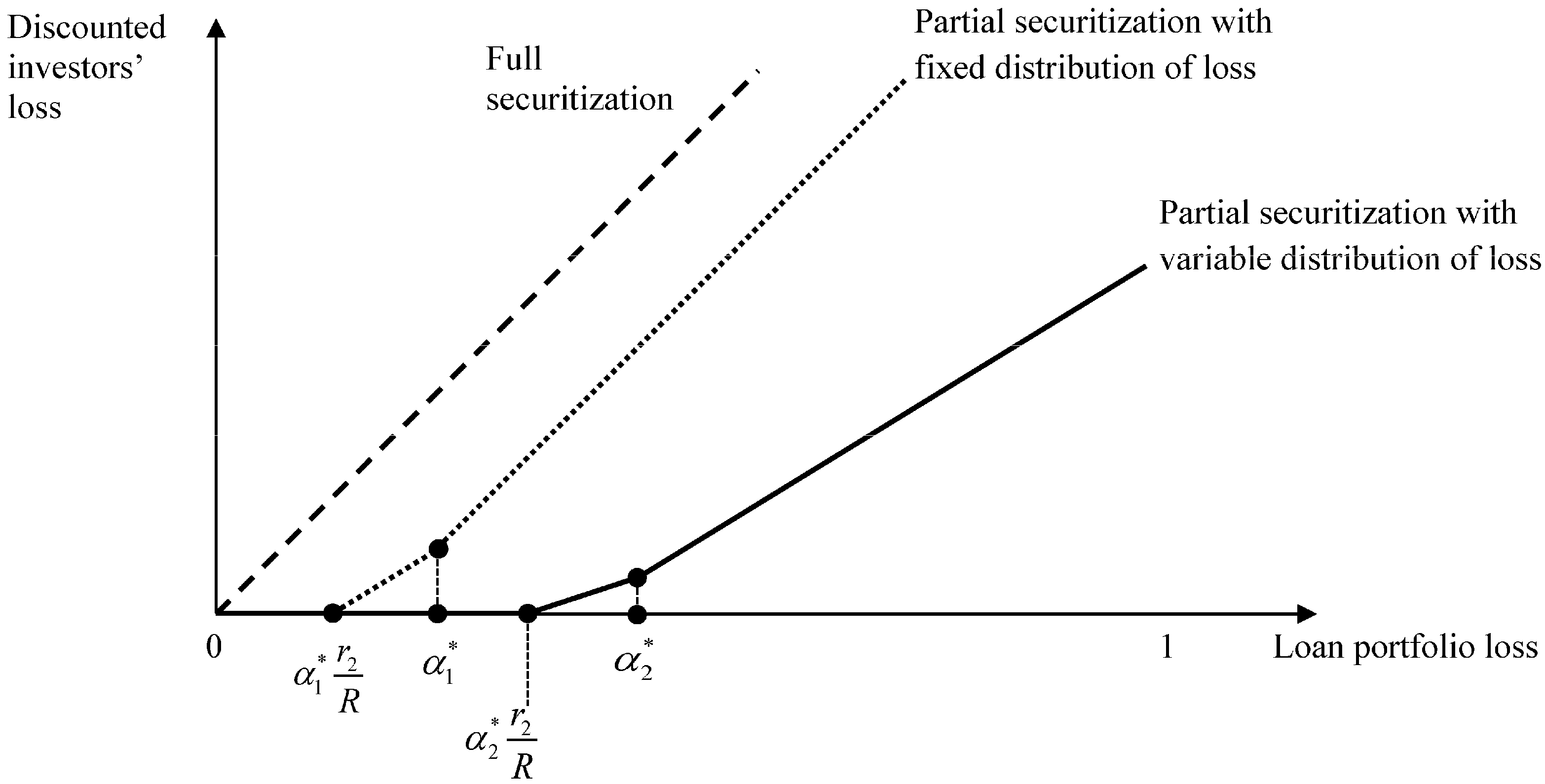
Figure 1. Optimal securitization contract with credit enhancement and different assumptions on the conditional distribution of loss. Investors’ discounted loss equals 0 when L < α 2 * r 2 R , equals ( L R α 2 * ( L ) r 2 1 + R ) when α 2 * r 2 R < L < α 2 * , and equals ( L α 2 * ( L ) ) + L R α 2 * ( L ) r 2 1 + R when L > α 2 * , and where α 2 * ( L ) = α 2 * + β L , 0 < β < 1 and α 2 * > α 1 * . When the conditional distribution of loss is not affected by effort, the optimal contract is an equity tranche equal to α 1 * .
Risks 05 00055 g001