Article

Interest Rates Term Structure under Ambiguity

1
Department of Statistics, University of Bologna, Via Belle Arti 41, 40126 Bologna, Italy
2
Prometeia, Via G. Marconi 43, 40122 Bologna, Italy
*
Author to whom correspondence should be addressed.
Risks 2017, 5(3), 50; https://doi.org/10.3390/risks5030050
Submission received: 30 July 2017 / Revised: 1 September 2017 / Accepted: 9 September 2017 / Published: 14 September 2017

Abstract

:
After financial crisis, the role of uncertainty in decision making processes has largely been recognized as the new variable that contributes to shaping interest rates and bond prices. Our aim is to discuss the impact of ambiguity on bonds interest rates (yields). Starting from the realistic assumption that investors ask for an ambiguity premium depending on the efficacy of government interventions (if any), we lead to an exponential multi-factor affine model which includes ambiguity as well as an ambiguous version of the Heath-Jarrow-Morton (HJM)model. As an example, we propose the realistic economic framework given by Ulrich (2008, 2011), and we recover the corresponding ambiguous HJM framework, thus offering a large set of interest rate models enriched with ambiguity. We also give a concrete view of how different simulated scenarios of ambiguity can influence the economic cycle (through rates and bond prices).
MSC:
91G30; 91B30; 91B70

1. Introduction

In a decision-making process, the lack of information influences the agent’s final choice. The uncertainty arising from this lack of information is called ambiguity. To understand what ambiguity is and why the world of finance looks at it with growing interest, in the following we propose a brief description of ambiguity and its evolution over time.
The intuition of ambiguity was initially developed by Knight (1921), starting from the distinction between risk and uncertainty. In Knight’s words:
“The practical difference between the two categories, risk and uncertainty, is that in the former the distribution of the outcome in a group of instances is known (either through calculation a priori or from statistics of past experience), while in the case of uncertainty this is not true, the reason being in general that it is impossible to form a group of instances, because the situation dealt with is in a high degree unique”.
If risk is that part of uncertainty that can be measured with objective likelihood laws, the “pure” uncertainty is instead linked to the uniqueness of situations analyzed. An instance of these situations is given by subjective choices. The so-called “Knightian uncertainty”(i.e., ambiguity) is not measurable, but nevertheless influences individual choices.
The concept of “Knightian uncertainty” was then developed by Ellsberg (1961) through two experiences, allowing him to remark that people prefer to bet on a known-probability lottery rather than bearing the uncertainty of an ambiguous result. A behaviour like this is called “ambiguity”.
Moreover, he showed us the so-called “Ellsberg paradox”: it consists of opting for the solution which offers the least perceived uncertainty, even if it leads to poorer payoff. Ellsberg explained this paradox with the ambiguity of information and he reckoned that the quality of given information (in terms of reliability, credibility, adequacy, and consensus upon it) could contribute to the degree of trust of each person, within the decision-making process. Thus emerged the concept of ambiguity as the result of two things—i.e., the quality of known information and the subjective perception of missing information.
After Ellsberg’s work, it has been increasingly recognized that the “awareness of missing information” (in Ellsberg’s words) influences individual attitude to bet. Some other relevant contributions to the foundational theory of ambiguity came from Gagliardini et al. (2009), showing that ambiguity plays a crucial role in decision-making processes (and so in people’s subjective choices). Fox and Tversky (1995) define the concept of comparative ignorance; i.e., ambiguity aversion arises when somebody has to decide in a context of events where he has very little—or no—experience. It is the same mechanism that leads, for example, sport experts to express forecasts only on sport events rather than different events.
In this work, we will focus on ambiguity in finance, with particular regard to the impact of ambiguity on bonds interest rates (yields). Starting from the realistic assumption that investors ask for an ambiguity premium depending on the efficacy of government interventions (if any), we extend the ambiguity element to Heath-Jarrow-Morton (HJM) approach, finding a closed form for interest rate term structure. This result involves the ambiguity contribution, and ultimately investors’ uncertainty about a country’s economic prospects.
We just gave a taste of how ambiguity can influence finance as well as other fields: from lotteries to weather forecasts, and even to forecasts on government interventions’ efficacy. The main central bank Governors acknowledge ambiguity as playing a role on economic measures: in December 2016, ECB Governor Mario Draghi said that “political uncertainty is dominant”; additionally, during the 7th OMFIF Meeting (2016) the Governor of the Bank of Italy Ignazio Visco said that “uncertainty is the hallmark of current global conditions […]. In its various dimensions—political, institutional, economic—uncertainty is playing a critical role in today’s global economic landscape”.
Indeed, ambiguity is a concrete factor arising from political situations and affecting government bonds’ yields: in Europe, examples of uncertainty-shaped events were the referendum in Italy about constitutional reforms (December 2016) and political elections in France (May 2017). Particularly, in Italy, just a few days before the vote for referendum, there was a raise of the spot yield in short-term government bonds, from −0.295% in October to −0.20%, as a possible lifting-up effect due to ambiguity1.
Other examples can be found today: post-Brexit scenarios still generate uncertainty, and in the US, Trump’s politics generate fears upon Fed movements on rates and hence a possible global financial crisis.
As shown in previous examples, ambiguity matters for choice. Thus, the decision model which best fits for ambiguity is the biseparable preference, as defined by Ghirardato et al. (2004). Based on the conditions satisfied in the decision-making process, the biseparable preference can be very useful in a context like the one we will borrow from Ulrich (2011) and Ulrich (2008), in which uncertainty can distort agents’ opinions and their utility. In fact, this kind of preference allows both for scenarios in which there is no ambiguity (the SEU model) and for others in which the agent has an attitude towards ambiguity.
In detail, the biseparable preference model can become one of the following well-known utility theories: the SEU, CEU, and MEU. The SEU is a theory set up by Savage (1954) that links utility functions to a probability distribution. Based on the hypothesis of rational individuals and considering a random event whose possible outcomes are x i , each with a utility U ( x i ) , individual choices will be given by the subjective expected utility, which is the expected utility weighted by the probability of each outcome ( P ( x i ) ). The agent who maximizes the expected subjective utility is defined as ambiguity neutral. The CEU is an extended version of the SEU theory. This theory was originally set up by Schmeidler (1989), and it is an expected utility computed thanks to the Choquet integral and to capacity2. Used together, these two tools allow for uncertainty about possible outcomes, as the capacity might also be an empty set. Thus, CEU is like an expected utility theory that allows for ambiguity. Another extended version of SEU is the MEU theory, set up by Gilboa and Schmeidler (1989). Here, the uncertainty among individuals is reached through multiple probabilities (one for each individual opinion) and preferences are represented through maximin function. Here the decision-maker’s information—which is incomplete and justifies his ambiguous belief—is explicitly consistent with multiple probabilities on the state space relevant to the decision at hand, usually related to the choice of the model. Model uncertainty refers to a situation where the decision-maker does not know the probabilistic model for the variables affecting the consequences of choices. A very similar motivation is that of the literature on decision-making under model misspecification doubts (see Hansen and Sargent (2008)) where a decision maker believes that data will come from an unknown member of a set of unspecified models near their approximating model. This approach leads to a decision problem with max-max preferences, as we will see in the example reported in Section 3.
Our work is organized as follows: Section 2 proposes an exponential affine multi-factor model including ambiguity in order to introduce ambiguity in the instantaneous term structure within the finite-state HJM framework. Section 3 provides an overview of the economic framework used as an example for our contribution. Ulrich (2011) built up an exponential affine theoretical model for zero coupon bond pricing which is affine on three factors. His model is particularly useful for our purposes because it provides a realistic economy as floor for the introduction of ambiguity from both theoretical and formal points of view. In fact, it focuses on the subjective perception of uncertainty and introduces it in an exponential affine form of zero coupon bond price. Using this economic background, we introduce the ambiguity contribution in the HJM interest rate framework and derive the main rates (forward instantaneous rate and forward and spot yields). In Section 3.2 we offer a sensitivity analysis of rates and zero coupon bond price for variations of the parameters used in the economic model. Finally, Section 4 concludes.

2. From a Multi-Factor Exponential-Affine Model to the HJM Model with Ambiguity

This paper aims to introduce ambiguity in the instantaneous term structure within the finite-state HJM framework. To do this, we define a multi-factor model, assuming that at least one of them is represented by the ambiguity. At first we state the presence of the ambiguity among the explicator factors as an a priori assumption that will be justified from an economical point of view in Section 3, specializing the multi-factors model into a three-factor model. Moreover, we assume to work in the family of exponential-affine multi-factor models where zero coupons bonds prices are allowed to be written in the following form:
B ( t , T ) = exp ( A ( t , T ) C ( t , T ) , X t ) ,
where . , . stands for the dot operator, A ( t , T ) R , C ( t , T ) R d and 1 is the d-dimensional unitary vector, while X t is a d-dimensional vector of factors which explains the instantaneous interest rate r t as an affine form of the factors3 whose Q -dynamic is
d X t = δ ( t , X t ) d t + σ ( t , X t ) , d W t
where ( W ) t is an n-dimensional Brownian motion, n n ^ d , where n ^ stands for the number of sources of risk4, in order to ensure the completeness of the market and the parameters δ ( t , X t ) R d , σ ( t , X t ) R d × n , are affine in the factors themselves; i.e.,
δ ( t , X t ) = b ( t ) + β ( t ) , X t σ ( t , X t ) σ ( t , X t ) = a ( t ) + α ( t ) , X t ,
where b ( t ) R d , a ( t ) , α ( t ) β ( t ) R d × d . Moreover, the instantaneous interest rate can be written as
r t = G ( t ) + J ( t ) , X t ,
where G ( t ) R , J ( t ) R d .
It is well known that under the previous assumptions of affine structures, the functions A ( t , T ) and C ( t , T ) are the solutions of the following system of differential equations:
t A ( t , T ) = 1 2 C ( t , T ) , a ( t ) C ( t , T ) b ( t ) , C ( t , T ) G ( t ) , A ( T , T ) = 0 t C ( t , T ) = 1 2 C ( t , T ) , α ( t ) C ( t , T ) β ( t ) , C ( t , T ) J ( t ) , C ( T , T ) = 0 ,
where 0 is the d-dimensional null vector.

Zero Coupon Bond Price Dynamics and HJM Model

Heath et al. (1992) developed a framework which unifies all the existing factor pricing models (e.g., Vasicek (1997), Cox et al. (1985), and Ho and Lee (1986) models), proposing an exogenous specification of the dynamic of the forward rates which depends only on the specification of the volatility function. The direct specification of the forward curve allows the problem related to the not enough flexible feature of the one factor models to be overcome in calibration with real data. In the HJM model, as placed in a Markovian setting by Musiela (1994), the state variable is the entire current yield curve, implying that any initial yield curve is generally consistent with the HJM model. On the other hand, since we work in a finite-dimensional state-space setting, our model has the disadvantage that not every initial yield curve is consistent with a given parametrization of the model. Furthermore, the disadvantage of the finite-dimensional state-space setting can also be positive in terms of numerical tractability. Furthermore, the proposed ambiguous version of the HJM model works in a very general setup which allows some well-known one factor models with ambiguity to be included as special cases; for example, it leads to the ambiguous version of the Ho–Lee model for a deterministic volatility function5.
Starting from the dynamics of f ( t , T ) under the historical P -measure; i.e.,
d f ( t , T ) = α ^ ( t , T ) d t + σ ^ ( t , T ) , d W ^ t ,
where ( W ^ ) t is the n-dimensional P -Brownian motion, while for every T, α ^ ( t , T ) R , σ ^ ( t , T ) R n are adapted stochastic processes, we impose the absence of arbitrage opportunities (AOA) through the steps explained hereafter.
Our starting point is the HJM equation under the P -measure, which can be written in integral form as follows:
f ( t , T ) = f ( 0 , T ) + 0 t α ^ ( s , T ) d s + 0 t σ ^ ( s , T ) , d W ^ s ,
where f ( 0 , T ) is the starting constant value for the forward instantaneous rate, α ^ ( t , T ) is the forward instantaneous rate drift, and σ ^ ( t , T ) is the forward instantaneous rate volatility at time t and for the maturity T.
Let us define the new Brownian motion W t under the Q -measure; i.e.,
d W t = d W ^ t + λ t d t ,
where λ t R n stands for the risk premium vector. Now let us express Equation (4) under the Q -measure as follows
f ( t , T ) = f ( 0 , T ) 0 t γ ( s , T ) , Γ ( s , T ) d s 0 t γ ( s , T ) , d W s ,
which corresponds to the forward structural HJM equation and where Γ ( t , T ) stands for the volatility of the zcb B ( t , T ) and γ ( t , T ) = Γ ( t , T ) T . Then, comparison of the forward structural HJM equation and Equation (4) implies that
σ ^ ( t , T ) = γ ( t , T ) ,
and the HJM structural equation under the Q -measure becomes
f ( t , T ) = f ( 0 , T ) + 0 t σ ^ ( s , T ) , s T σ ^ ( s , u ) d u d s + 0 t σ ^ ( s , T ) d W s .
On the other hand, under the historical measure P , the AOA implies the following:
f ( t , T ) = f ( 0 , T ) + 0 t σ ^ ( s , T ) , s T σ ^ ( s , u ) d u d s + 0 t σ ^ ( s , T ) , λ s d s + 0 t σ ^ ( s , T ) , d W ^ s .
Therefore, by comparing the HJM equation on the P -measure and the corresponding structural equation on the Q -measure, we recover the HJM drift condition; i.e.,
0 t α ^ ( s , T ) d s = 0 t σ ^ ( s , T ) , s T σ ^ ( s , u ) d u d s + 0 t σ ^ ( s , T ) , λ s d s ,
which assures the AOA and explains the drift as a function of the volatility. Hence, we can explicitly retrieve the HJM condition on drift which assures for the AOA; i.e.,
α ^ ( t , T ) = σ ^ ( t , T ) , t T σ ^ ( t , v ) d v + λ t ,
for each T [ 0 , T t ] and t [ 0 , T ] . Therefore, the choice of the volatility function and then of the zero coupon bond volatility function allows us to completely specify the HJM model. Thus, we have a bridge connecting the previously discussed multi-factor exponential affine model, which includes the ambiguity factor, and the HJM model which can be specified in order to ensure the absence of arbitrages and to include the impact of ambiguity as well.
Moreover, given the exponential-affine representation of zero coupon bond prices discussed before, we are now able to find the zero coupon bond B ( t , T ) dynamics. To get to this point, let us apply Itô’s lemma:
d B ( t , T ) = B ( t , T ) t ( t , X t ) d t + i = 1 d B ( t , T ) X t i ( t , X t ) d X t i + + 1 2 i = 1 j = 1 d 2 B ( t , T ) X i X j ( t , X t ) d X i , X j ,
where the dth component of X is the ambiguity factor. In our model specification, we explain two cases based on Brownian motion components’ dependence; i.e.,
  • absence of correlation among Brownian motions;
  • dependence or presence of some correlation among Brownian motions.
    We prove the following proposition.
Proposition 1.
The HJM model under ambiguity coherent with the multi-factor exponential affine model discussed in the previous section is defined by the following choice of volatility function:
σ ^ ( t , T ) = Γ ( t , T ) T ,
where Γ ( t , T ) = B ( t , T ) C ( t , T ) , σ ( t , X t ) .
Proof. 
Given the exponential-affine representation of zero coupon bond prices, it is straightforward to compute the derivatives of zcb’s price; i.e.,
B ( t , T ) t ( t , X t ) = B ( t , T ) [ A ( t , T ) C ( t , T ) · X t ] B ( t , T ) X t i ( t , X t ) = B ( t , T ) C i ( t , T ) 2 B ( t , T ) X i X j ( t , X t ) = B ( t , T ) C i ( t , T ) C j ( t , T ) .
Finally we have the thesis after substituting in Equation (5). ☐
In the next section, we consider an example of the previous multi-factor exponential-affine model which refers to the Ulrich (2011) model, whose economic framework is deeply discussed along with the role of ambiguity.

3. A Three-Factor Exponential Affine Model: The Economic Framework

Here we give an overview of Ulrich (2011) and Ulrich (2008) proposed as an example of the previously discussed multi-factor exponential affine model which includes ambiguity in a well-specified economic framework.
Ulrich starts with this question: do government interventions influence consumptions and real interest rates? If we use the Ricardian equivalence in our reasoning, then we should answer “no”, because every announcement of political reform would be offset by individuals who would anticipate its effect. Hence, the government multiplier would be zero. However, reality would lead us to answer “yes” to Ulrich’s starting question: in fact, both consumptions and interest rates play a fundamental role in a country’s economy, and often governments introduce reforms in order to target exactly these variables (for example, after the financial crisis of 2007 and following years, many national governments had to face the problem of low consumptions and tried to reform in order to increase these variables). The distance between the neo-classical economic theory and reality moves to investors’ opinion in terms of uncertainty. In his model, two types of uncertainties are introduced in the zcb pricing:
  • the known-unknown, which reflects the dispersion among investors’ opinions about validity of Ricardian equivalence. This refers to a policy intervention uncertainty because it reflects the attempt of government to systematically change the consumption growth;
  • the unknown-unknown, which represents uncertainty about the future effectiveness of a government’s interventions on future consumption. This uncertainty is harder to measure, and can be numerically translated into a multiplier uncertainty which is directly proportional to the growth of economy and the inflation.
Given this premise, the model is made explicit in terms of a set of processes for consumption growth, including the model assuring the Ricardian equivalence. Under the last one (i.e., the reference model), we work on a complete filtered probability space ( Ω , F , Q 0 ) , and the dynamics of consumption’s growth is given by
d ln ( c t ) = ( c 0 + z t ) d t + σ c d W t c ,
where c 0 > 0 represents consumption’s growth rate at time t = 0 , ( W c ) t is a one-dimensional Q 0 -Brownian motion, and z is an Ornstein–Uhlenbeck process which describes economic cycle, whose dynamics is:
d z t = k z z t d t + σ z d W t z ,
where k z < 0 and finally σ c and σ z stand for the volatilities of consumption’s growth and economic cycle, respectively.
As a starting point, we assume that the Ricardian equivalence holds true: therefore, political reforms have no effect on consumption and the government spending multiplier is zero. In terms of the formal expression of the model, this means that real interest rate volatility depends entirely on expected consumptions’ growth volatility and W c is orthogonal to W z .
In order to introduce uncertainty about the correctness of Ricardian equivalence, we formalize the Brownian motion d W z as consisting of two components (independent between them):
d W t z = ρ ¯ d W t z ^ + 1 ρ ¯ 2 d W t G ,
where d W t z ^ describes the evolution of technology within the economy while d W t G describes the net effect of political reforms introduced in the economy6.
Moreover, we assume that every economic agent knows their own utility at time t, which depends on private consumption only and then it is not ambiguous a priori; i.e.,
U ( c t ) = E t Q 0 t e ρ ( s t ) ln ( c s ) d s ,
where ρ R + stands for the subjective discount factor. In order to introduce the uncertainty component, recall that every economic agent within the economy does not believe totally in the Ricardian equivalence, thinking that actually the government might seek to influence their consumptions. This translates into a net effect of governments policies given by d W t G that will vary from agent to agent, based on their opinions related to the government announcements.
In other words, a non-Ricardian policy model accounts for a non-zero conditional expected growth rate on d W t G ; i.e.,
d W t G = d W t G , h G + h t G d t ,
where the multiplier policy h t G 0 stands for the instantaneous deviation of economic agents’ opinion from Ricardian equivalence. We observe that if it tends to zero then the investor’s opinion will be closer and closer to believing in Ricardian equivalence (so it is like the distortion also tends to zero). The multiplier is unobserved by the agent, and it is an endogenous outcome of the government’s decision problem. On the other hand, d W t G , h G stands for the shock on government’s policies under the distorted measure Q h G .
From Equation (7), we can get the distorted dynamics of the economic cycle, i.e.,
d z t = ( k z z t + σ z 1 ρ ¯ 2 h t G ) d t + σ z ( ρ ¯ d W t z ^ + 1 ρ ¯ 2 d W t G , h G ) ,
supporting the belief in a systematic impact of government’s policy on the drift of z.
Now, let us move to the government’s point of view: as a matter of fact, it must face the problem of maximizing economic agents’ utility, choosing its intervention among a set of policies with different degrees of distance from Ricardian equivalence; i.e.,
max ( h t G ) H E t Q 0 t e ρ s ln ( c s ) d s u . c . ( 6 ) , ( 8 ) u . c . 1 2 ( h t G ) 2 d t A η t 2 d t ,
where 1 2 ( h t G ) 2 d t E t h G d ln d Q h G d Q 0 and h t G expresses the distance between distorted opinion and benchmark (i.e., Ricardian) opinion. Moreover, H represents the set of policies that the government could implement7, A > 0 represents the number of non-Ricardian models, which is the complexity of H , while η t 2 d t shows the variation across time of the set of non-Ricardian models. This approach extends the rational expectation model to acknowledge fear and model misspecification, where the government’s decision problem endogenizes the agent’s preferences which are of max-max type8.
Stating that the government can observe the number of policies but does not know the statistical model describing this set of models, we can write down their dynamics; i.e.,
d η t = ( a η + k η η t + σ η L t ) d t + σ η a η k η d W t η , h η ,
where a η > 0 , k η < 0 , a η k η = E Q h G ( η t ) 9 and L t represents the multiplier uncertainty which will be specified in the following. We observe that we account here for a perturbation h η characterizing the multiplier uncertainty, whose optimal solution for the government’s problem is h t η = L t η t > 0 .
We observe that from the previous assumption it comes that the government knows how many policies are compatible with the Ricardian equivalence. With this information, the government’s problem of maximization can be solved with Hamilton-Jacobi-Bellman (HJB) differential approach and the optimal solution is:
h t G d t = 2 A η t d t m G η t d t ,
where 2 A m G for definition.
Thanks to this solution, we can again write the distorted economy dynamics:
d z t = k z z t + σ z 1 ρ ¯ 2 m G η t d t + σ z ( ρ ¯ d W t z ^ + 1 ρ ¯ 2 d W t G , h G ) d η t = ( a η + k η η t + σ η L t ) d t + σ η a η k η d W t η , h η
The optimal solution leads us to some interesting considerations:
  • In a non-Ricardian world, if the government acts in a “benevolent” way (i.e., introducing policies which maximize economic agents utility), consumption’s instantaneous rate of growth will increase based on the following factor:
    σ z 1 ρ ¯ 2 m G η t d t > 0 .
  • If the government instead acts in a “malevolent” way (i.e., minimizing economic agents’ utility—in this way, the government does not act for their sake), the sign of the intervention will be opposite to the one we saw as optimal solution (see Equation (9) ).
Up to this point, we have discussed the first kind of uncertainty (the “known-unknown”), but as said at the beginning, there is also another type of uncertainty called “unknown-unknown”, related to the efficacy of the government’s interventions from the government’s perspective and which may be identified more precisely as multiplier ambiguity. It is more difficult to deal with this kind of uncertainty, because as we saw, it is not measurable. To find a proper measure for it, we use a proxy, which is a government multiplier; i.e., we assume that there is a factor L driving the distance between the reference model for η (i.e., the model with zero perturbation, h η = 0 ) and the distorted ones. The higher the uncertainty about whether the interventions will sort their effect, the higher the multiplier h η . The dynamics of this uncertainty is:
d L t = ( a L + k L L t ) d t + σ L a L k L d W t L ,
where a L > 0 , k L < 0 and a L k L = E Q h η ( L t ) 10.
We are talking about government interventions and economic agents’ utility, and we are interested in discussing wether investors’ expectations will be incorporated in real interest rates. Ulrich (2011) proves that real zero coupon bond prices can be written in the exponential affine form, and matches the previously discussed multi-factor exponential affine modeling; i.e.,
B ( t , T ) = exp ( A ( τ ) C ( τ ) , X t ) ,
where τ = T t and,
C ( τ ) = [ C z ( τ ) C η ( τ ) C L ( τ ) ] X t = [ z t η t L t ] .
Moreover, from Equation (10), we can derive real bond yield:
B ( t , T ) = exp τ y t ( τ ) y t ( τ ) = l n B ( t , T ) τ .
Let us have a look to each component of the yield y t . First, we observe that C z ( τ ) depends only on the economic cycle variable z t , and more precisely, it has a direct effect on the level of real interest rates. So, if the economic cycle expands ( z t increase), also real interest rates will grow in order to offset the investors’ propensity to save money and spend it in the future, thus leading to a decrease in bond price. Its expression is:
C z ( τ ) = e k z τ 1 k z R , C z ( 0 ) = 0 , C z ( ) = 1 k z < 0 .
Moreover, C η ( τ ) describes the known unknown uncertainty component and its link to consumption. It is represented in the following analytical form:
C η ( τ ) = m G 1 ρ ¯ 2 σ z k z k η 1 e k η τ + k η ( e k z τ e k η τ ) ( k z k η ) .
Finally, C L ( τ ) describes the impact of the unknown unknown uncertainty on real yields; i.e.,
C L ( τ ) = m G 1 ρ ¯ 2 σ z σ η k z g ( τ ) g ( τ ) = 1 e k L τ k L k η + e k η τ e k L τ k η ( k L k η ) + e k z τ e k L τ ( k z k L ) ( k z k η ) e k η τ e k L τ ( k η k L ) ( k z k η ) .

3.1. A Three-Factor Exponential Affine Model: HJM Model under Ambiguity

Our starting point is is a multi-factor model which expresses zero coupon bond (hereinafter zcb) price in affine exponential form, suitable to HJM framework. Later, we moved to the definition of the zcb volatility using stochastic analysis tools, in order to reach the representation of the forward instantaneous rate. Now, focusing on the Ulrich (2011) model we discussed in the previous section on how to write the zcb price under distorted measure Q h (i.e., with ambiguity) as in (10) where the dynamic of the factor matches Equation (2) for
δ ( t , X t ) = k z z t + σ z 1 ρ ¯ 2 m G η t a η + k η η t + σ η L t a L + k L L t W ¯ t = W t z ^ W t G , h G W t η , h η W t L σ ( t , X t ) = σ z ρ ¯ σ z 1 ρ ¯ 2 0 0 0 0 σ η a η k η 0 0 0 0 σ L a L k L ,
where ( W ¯ ) t is a 4-dimensional Q h -Brownian vector and they allow for an affine decomposition as in (3), where
b ( t ) = [ 0 a η a L ] β ( t ) = k z 0 0 σ z 1 ρ ¯ 2 m G k η 0 0 σ η k L a ( t ) = σ z 2 0 0 0 σ η 2 a η k η 0 0 0 σ L 2 a L k L α ( t ) = 0 ,
where 0 R 3 × 3 is the zero matrix. Moreover, since r t = ρ + c 0 + σ c 2 2 + z t , we have
J ( t ) = [ 1 0 0 ] G ( t ) = ρ + c 0 + σ c 2 2 .
Finally, we observe that—given the homogeneous-in-time property of the model at hand—the real price of a zcb is well defined by the solutions of the following system:
τ A ( τ ) = b ( t ) , C ( τ ) 1 2 C ( τ ) , a ( t ) C ( τ ) G ( t ) , A ( 0 ) = 0 τ C ( τ ) = β ( t ) , C ( τ ) 1 2 C ( τ ) , α ( t ) C ( τ ) J ( t ) , C ( 0 ) = 0 ,
where τ = T t and 0 is the d-dimensional null vector.
We point out that the explicit solution for A ( τ ) can be recovered by the following integration process:
A ( τ ) = ρ + c 0 + σ c 2 2 τ + 1 2 σ z 2 0 τ C z 2 ( u ) d u + σ η 2 a η k η 0 τ C η 2 ( u ) d u + + σ L 2 a L k L 0 τ C L 2 ( u ) d u + a η 0 τ C η ( u ) d u + a L 0 τ C L ( u ) d u .
Considering that the variables z , η , L depend on a 4-dimensional Brownian vector, we will find interesting results in the case of dependence among Brownian motions and an absence of correlation between them.

3.1.1. Absence of Correlation among the Sources of Risk

Proposition 2.
Assuming an absolute absence of correlation among Brownian motions involved in this model means no interrelation among shocks. In other words, the shock on one variable does not affect the others. This is a useful case to observe shock’s consequences, ceteris paribus. In this case, the price B ( t , t + τ ) dynamics is:
d B ( t , t + τ ) = B ( t , t + τ ) [ Δ ( τ , z , η , L ) d t + Γ ( τ , z , η , L ) , d W ¯ t ]
where
Δ ( τ , z , η , L ) = ( τ A ( τ ) + A ( τ ) ) z t e k z τ + η t m G 1 ρ ¯ 2 σ z k z e k η τ k z e k z τ k η e k η τ k z k η + L t m G 1 ρ ¯ 2 σ z σ η k z [ e k L τ k η + k η e k η τ k L e k L τ k η ( k L k η ) + + k z e k z τ k L e k L τ ( k z k L ) ( k z k η ) k η e k η τ k L e k L τ ( k η k L ) ( k z k η ) ] + 1 2 C z 2 ( τ ) σ z 2 + + C z ( τ ) k z z t + σ z 1 ρ ¯ 2 m G η t + 1 2 C η 2 ( τ ) σ η 2 a η k η + + C η ( τ ) ( a η + k η η t + σ η L t ) + 1 2 C L 2 ( τ ) σ L 2 a L k L + C L ( τ ) ( a L + k L L t ) Γ ( τ , z , η , L ) = [ C z ( τ ) σ z ρ ¯ C z ( τ ) 1 ρ ¯ 2 C η ( τ ) σ η a η k η C L ( τ ) σ L a L k L ] W ¯ t = [ W t z ^ W t G , h G W t η , h η W t L ]
Proof. 
The thesis follows from a direct calculous of Itô’s lemma as detailed in Equation (5). ☐

3.1.2. Dependence among the Sources of Risk

By assuming the dependence among Brownian motions W t z ^ , W t G , h G , W t η , h η , and W t L , we mean a realistic scenario in which a shock on one variable may also affect the other variables through a certain degree of correlation.
In terms of mathematical computations, we must account for the correlations between couples of Brownian motions. Hereafter, these correlations will be identified as follows:
corr ( W t z ^ , W t η , h η ) = α corr ( W t G , h G , W t η , h η ) = α ¯ corr ( W t z ^ , W t L ) = γ corr ( W t G , h G , W t L ) = γ ¯ corr ( W t L , W t η , h η ) = ω
However, we assume that
corr ( W t z ^ , W t G , h G ) = corr ( W t G , h G , W t z ^ ) = 0
because, by the starting assumption of the model, the economic cycle stochasticity is a linear combination of these two Brownian motions, orthogonal to each other. This characteristic represents the thick link between the volatility of economic cycle and shocks on consumption in the context of greater or lesser ambiguity.
Proposition 3.
Under the assumptions of correlation among Brownian motions involved in this model as outlined above, the dynamic of B ( t , T ) is
d B ( t , t + τ ) = B ( t , t + τ ) [ Δ ^ ( τ , z , η , L ) d t + Γ ^ ( τ , z , η , L ) , d W t ˜ ]
where
Δ ^ ( τ , z , η , L ) = ( τ A ( τ ) + A ( τ ) ) z t e k z τ + η t m G 1 ρ ¯ 2 σ z k z e k η τ k z e k z τ k η e k η τ k z k η + L t m G 1 ρ ¯ 2 σ z σ η k z e k L τ k η + k η e k η τ k L e k L τ k η ( k L k η ) + k z e k z τ k L e k L τ ( k z k L ) ( k z k η ) + k η e k η τ k L e k L τ ( k η k L ) ( k z k η ) + 1 2 C z 2 ( τ ) σ z 2 + C z ( τ ) k z z t + σ z 1 ρ ¯ 2 m G η t + + 1 2 C η 2 ( τ ) σ η 2 a η k η + C η ( τ ) a η + k η η t + σ η L t + 1 2 C L 2 ( τ ) σ L 2 a L k L + + C L ( τ ) a L + k L L t + C z ( τ ) C η ( τ ) σ z σ η a η k η ( ρ ¯ α + α ¯ 1 ρ ¯ 2 ) + + C z ( τ ) C L ( τ ) σ z σ L a L k L ( ρ ¯ γ + γ ¯ 1 ρ ¯ 2 ) + C η ( τ ) C L ( τ ) σ η σ L ω a η a L k η k L Γ ^ ( τ , z , η , L ) = Γ ( t , z , η , L ) C z 2 ( τ ) σ z 2 ρ ¯ 2 + C z 2 ( τ ) σ z 2 ( 1 ρ ¯ 2 ) + C η 2 ( τ ) σ η 2 a η k η + C L 2 ( τ ) σ L 2 a L k L + Ξ ( τ ) Ξ ( τ ) = C z ( τ ) C η ( τ ) σ z σ η a η k η ρ ¯ α + α ¯ 1 ρ ¯ 2 + C z ( τ ) C L ( τ ) σ z σ L a L k L ρ ¯ γ + + γ ¯ 1 ρ ¯ 2 + C η ( τ ) C L ( τ ) σ η σ L ω a η a L k η k L
W ˜ t = C z ( τ ) σ z ρ ¯ W t z ^ Γ ^ ( t , z , η , L ) + C z ( τ ) σ z 1 ρ ¯ 2 W t G , h G Γ ^ ( t , z , η , L ) + C η ( τ ) σ η a η k η W t η , h η Γ ^ ( t , z , η , L ) + + C L ( τ ) σ L a L k L W t L Γ ^ ( t , z , η , L )
Proof. 
We observe that if we compared the dynamic of zcb computed in case of independence of the Brownian motions to the dependent case, there is one more term in the price expression. This term is the one corresponding to the mixed derivatives among factors (i.e., Ξ ( τ ) ). Moreover, given the definition of a new Brownian motion W ˜ obtained by linearly combining the one-dimensional Brownians, the thesis follows from a direct calculous of Itô’s lemma as detailed in Equation (5). ☐
The analytic form through which we expressed the zero coupon bond volatility is a further help towards HJM forward instantaneous rate computation. To this end, we will need the derivative of the zero coupon bond volatility with respect to the maturity.

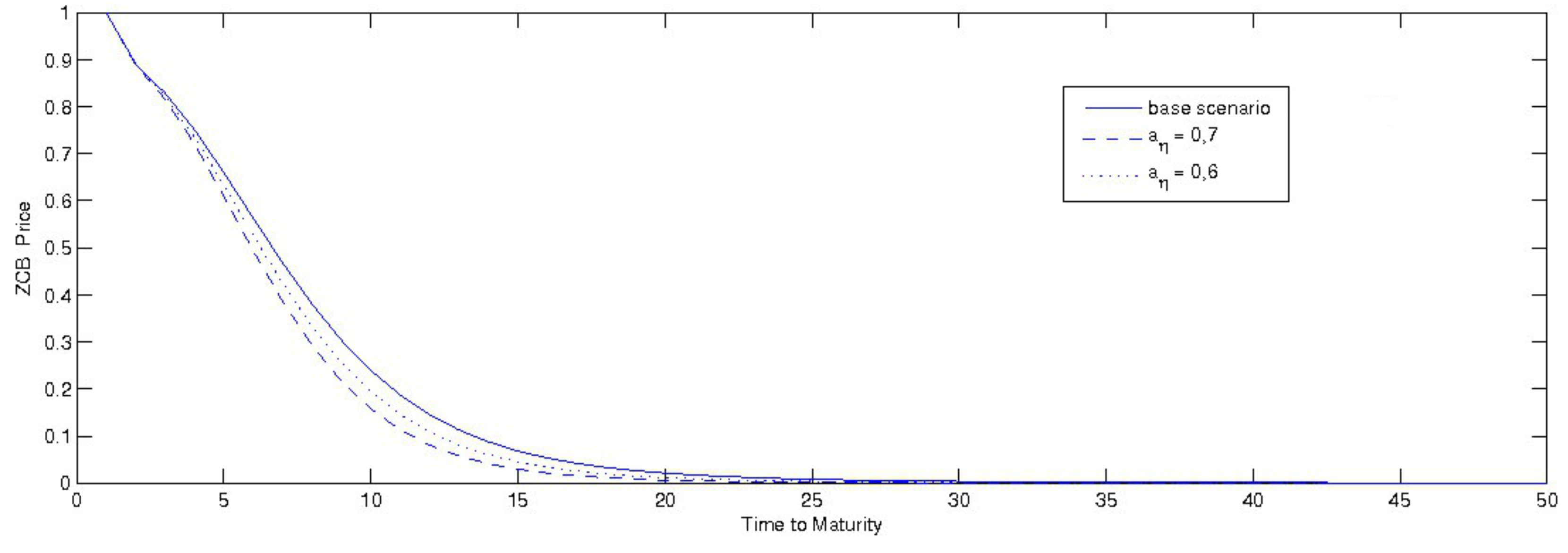
3.2. Sensitivity Analysis

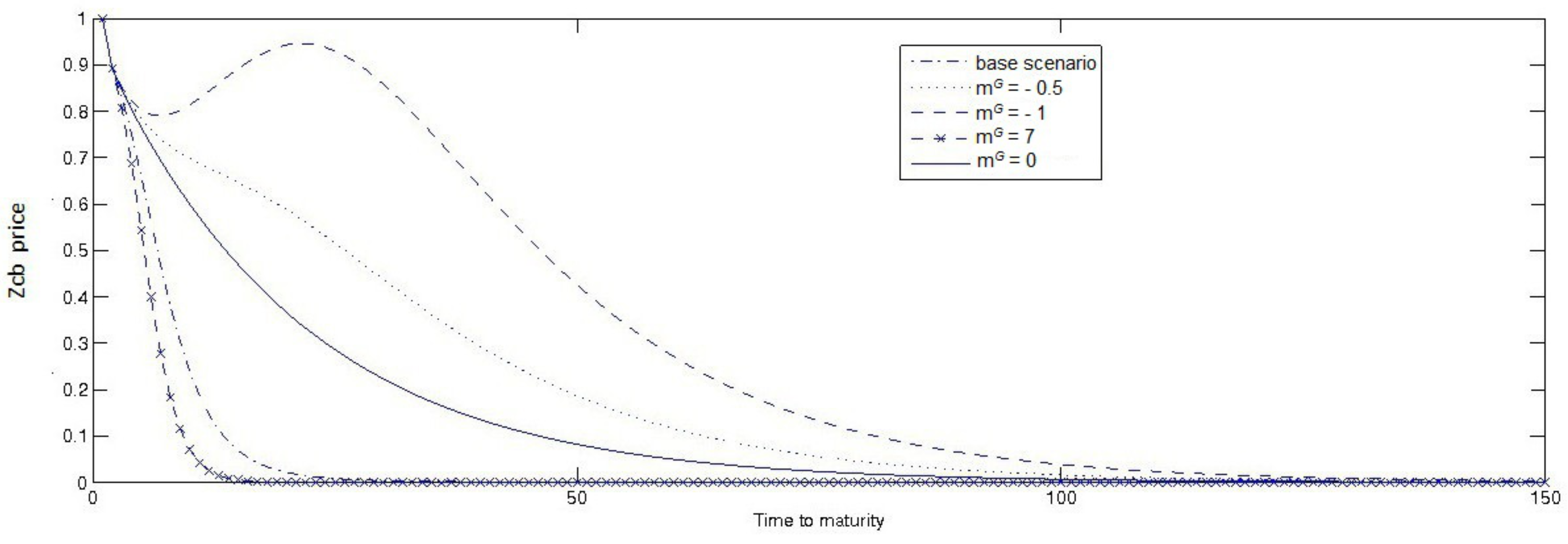
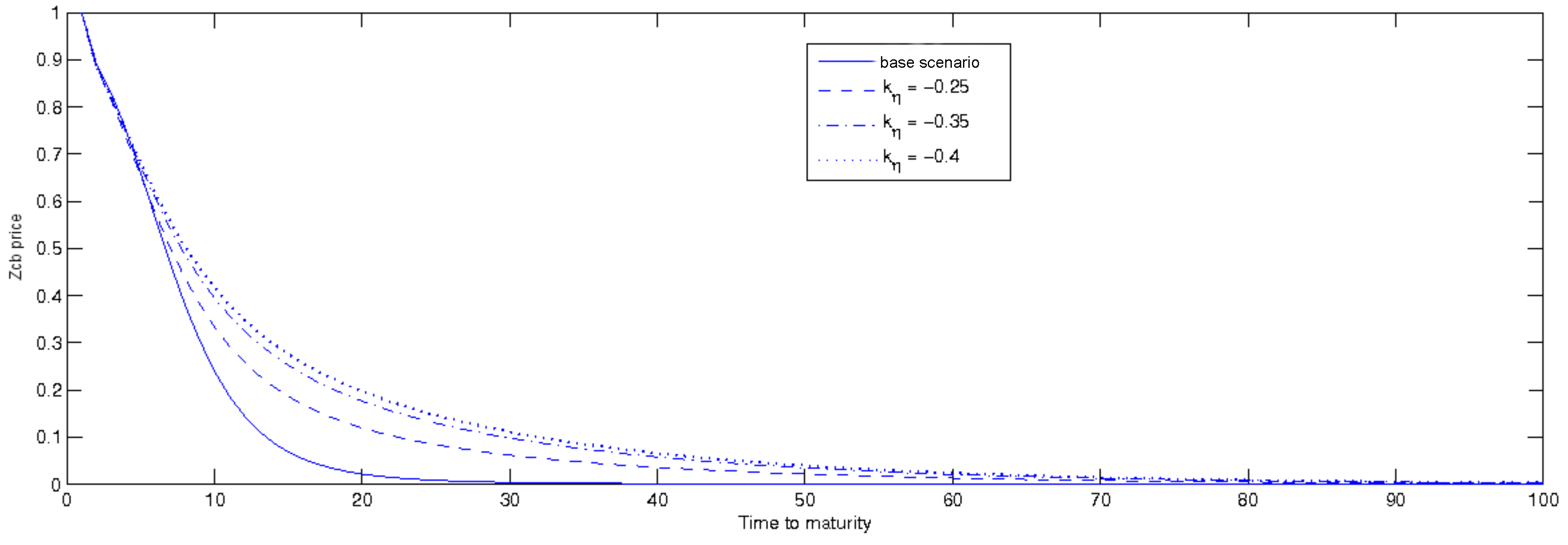
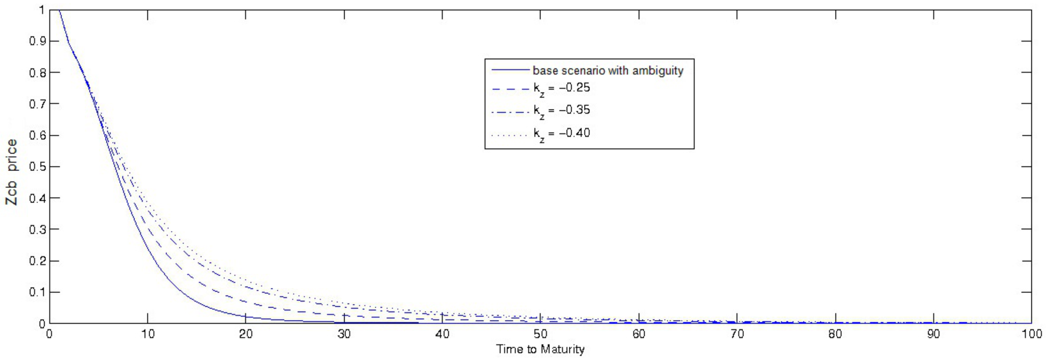
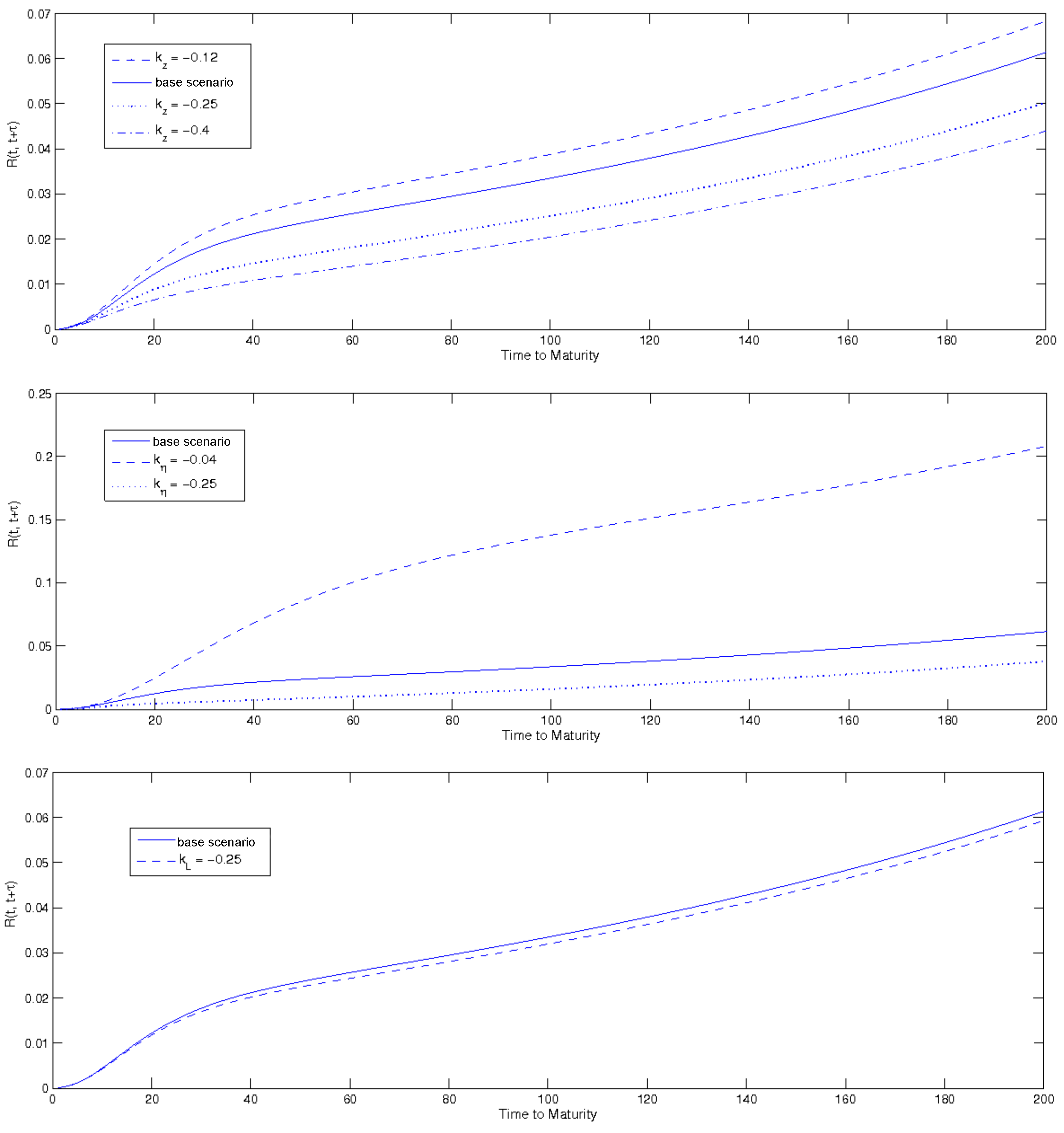
3.2.1. Zcb Real Price: A Sensitivity Analysis

In this section we will introduce our sensitivity analysis of zero coupon bond price. The baseline scenario built and used in the following charts corresponds to a case of normal ambiguity, which is assumed to be related to m G = 3 , with other parameters calibrated as follows:
  • correlation coefficients are all equal to zero (case of independence of Brownian motions);
  • both kinds of perceived ambiguity ( a η and a L ) are equal to an average value (i.e., 0.5);
  • the volatility parameters have been calibrated on low but realistic values: σ z = 0.003 , σ η = 0.005 , σ L = 0.006 ;
  • the coefficients k z , k η , and k L have been calibrated on −0.1, −0.15, −0.05.
Figure 1 shows the impact of government actions on zero coupon bond price. The set of policies from which the government may choose for its intervention is represented by the parameter m G : the larger the set, the higher the ambiguity. Besides, the parameter m G also means the attitude towards investors and consumers shown by the government through its interventions:
  • m G > 0 
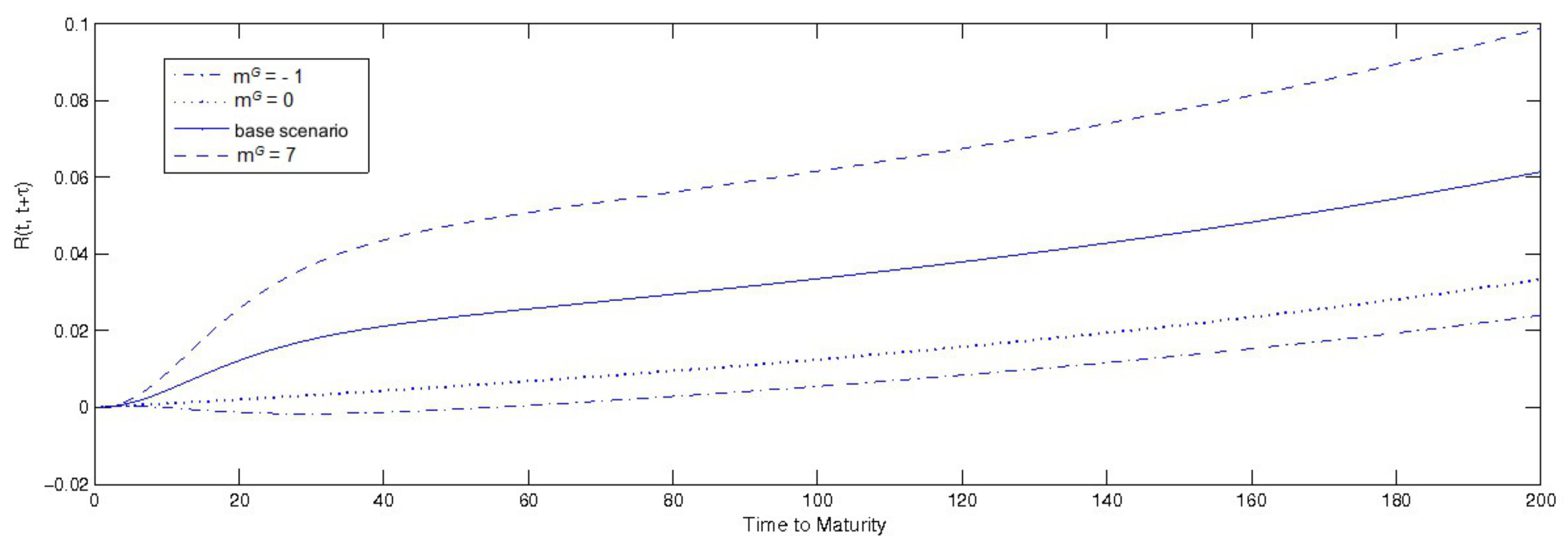
: the government action maximizes economic agents utility, and thus is “benevolent”;
  • m G = 0 : the government does not act to influence economic agents’ utility, behaving as described in the Ricardian equivalence. This is the case of no ambiguity;
  • m G < 0 : government interventions minimize economic agents’ utility. In other words, government actions are “malevolent”; i.e., harmful for the economic agents in the economy.
Figure 1 shows a sensitivity analysis of the zero coupon bond price on different attitudes of the government. Compared with the base scenario, a benevolent government (a larger m G ) reduces zcb volatility. A malevolent action instead brings the government bond to higher levels of volatility, especially on short time horizons.
These conclusions are realistic: in fact, what investors fear are government actions potentially injurious to their income, their wealth, and ultimately their choices of consumption and investment. Translated into ambiguity, this fear increasingly impacts zcb prices the more the government introduces inefficient policies or policies with actual negative effects.
Figure 2 shows the impact of ambiguity perceived by investors (represented by a η parameter) on the zcb price. The base scenario considered here represents the general case in which the government acts for the economic agents’ sake (i.e., for higher consumption rates), but in the context of some uncertainty. Nevertheless, with this benevolent behaviour of government, a higher a η (like the one represented in Figure 2), ceteris paribus, means higher dispersion among investors’ opinion on whether government acts with respect to Ricardian equivalence, with an overall reducing effect on zcb price.
So far, we have analysed two interesting factors and the role they play in shifting the zero coupon bond curve as a consequence of the model we built, which is also applicable to reality. An example could be the post-Brexit scenario and its effects on the English economy. What would investors have expected from the new government? A pool of expansive policies to influence consumptions or a pool of policies that would have raised taxes in order to drain financial resources for the standalone-Great-Britain? Other examples borrowed from the current reality are France and Italy during the last election period. Both countries faced growing uncertainty: on one hand, uncertainty in France regarding who would have been elected as Prime Minister, among candidates with very different positions. On the other hand Italy, facing uncertainty after the Prime Minister’s resignation.
To better understand how different simulated scenarios of ambiguity can influence the economic cycle, we develop a model in which GDP is endogenously determined as in Ilut and Schneider (2014), and the effects of ambiguity on bond prices given GDP will be emphasized. We consider three periods which precede or follow special events such as Brexit, the elections of the Prime Minister in France, and the referendum about the constitutional reform in Italy, and quantitatively calculate how much change in ambiguity is needed to explain movements in bond prices for simulations in Figure 1. In order to match the model with data, it is advantageous if one proxies the amount of this uncertainty by an observable and government-related intervention process which is linear in expected GDP growth. To this aim, we use ECB Survey of Professional Forecasters (SPF) data on the GDP growth, and we assume that the state variables z and η coincide with the demeaned11 one-quarter-ahead median and standard deviation forecast of GDP growth. Finally, we compare the realized model for z—estimated with a one-step Maximum Likeihood (ML) method—to the expected one recovering the corresponding government multiplier. For simplicity, we assume the absence of technology shock(i.e., ρ ¯ = 0 ), and we proxy a η with the realized standard deviation of GDP growth.
Empirical coefficients resulting from estimations reported in Table 1 can be discussed in view of what is shown in previous figures. In fact, if we relate estimated coefficients with those explained by the curves represented in Figure 1 and Figure 2, we find that the Brexit case and the French case place in a context of lower/higher m G , respectively, if compared to the base scenario, but increasing in the post-Brexit period (consistent with a more benevolent government) while a η is lower than the base scenario and stable in the post-Brexit (supporting a scenario which is stable in the dispersion of the investors’ opinions). On the other hand, Italy’s case shows higher and decreasing m G , consistent with a slightly less benevolent government, and higher a η , mirroring a real raise in investors’ uncertainty.
Regarding the Brexit example, we know that after the “Leave” vote won in the Brexit referendum, it opened a completely unexpected situation involving politics, society, and most of all, economy. Thus, Brexit is the best example of how ambiguity matters in the world in which we live. Estimated coefficients (particularly m G ) place the Brexit case moving from a context of low ambiguity to a case of normal ambiguity (represented by the base scenario) in the post-Brexit, still remaining stable in perceived investors’ uncertainty.
Compared with the clear Brexit case, the other two examples (Italy and France) show contrasting results, but are nonetheless meaningful. The couple of coefficients estimated from data collected before and after Italy’s vote on constitutional reform is consistent with a context of larger ambiguity perceived by investors, even though parameter m G would suggest lower ambiguity. This contrast might find its explanation if we think that some months before the vote, the Italian Prime Minister had some promise of resignation in the event of a bad referendum result (which actually occurred, leading to his resignation). So, in the Italian case, uncertainty in terms of greater dispersion in investors’ beliefs came after the referendum, because nobody really expected the Prime Minister’s resignation in a fragile moment for Italy’s economy as justified by a diminishing of m G . Last but not least, the elections in France: based on available data12 we can see that coefficients which came out of the estimation process are consistent with an ambiguity-based scenario, as described in this paper. In fact, uncertainty about which party would have won elections translated into a huge m G (i.e., in many more policy models to choose from) for France’s new government.
In the following figures we explain the impact of each of the other parameters included in the model having an impact on the zcb price volatility, considering the base scenario as a normal benchmark.
Figure 3 shows that a greater economic cycle volatility causes a lower zcb volatility and a greater known-unknown ambiguity (Figure 4). This different consequence is due to the prevalence between effects. In fact, in the case of the economic cycle (Figure 3), a greater volatility means a growth in the economy (as assumed by the underlying model), and thus a better individual welfare. These two positive effects will be transferred to the zero coupon bond as lower volatility. On the other side, Figure 4 shows that a greater known-unknown ambiguity volatility implies, ceteris paribus, a greater zcb volatility. This effect is because of the predominance of the stochastic volatility component on the drift inside the zcb dynamics.
Regarding the effects of different levels of unknown-unknown ambiguity volatility ( σ L ), there are no considerable variations in the zcb price. This behaviour is eloquent with the nature of unknown-unknown ambiguity, which is latent and not directly observable.
Moreover, we studied the effects of different levels of k z and k η parameters on the zcb13.
As we can see from Figure 5 and Figure 6, with lower levels of each of the considered parameters, we get a higher zcb curve. This consequence means a larger zcb volatility. Thus, also in this case, the volatility factor inside the dynamics weighs more, determining the effects we see.

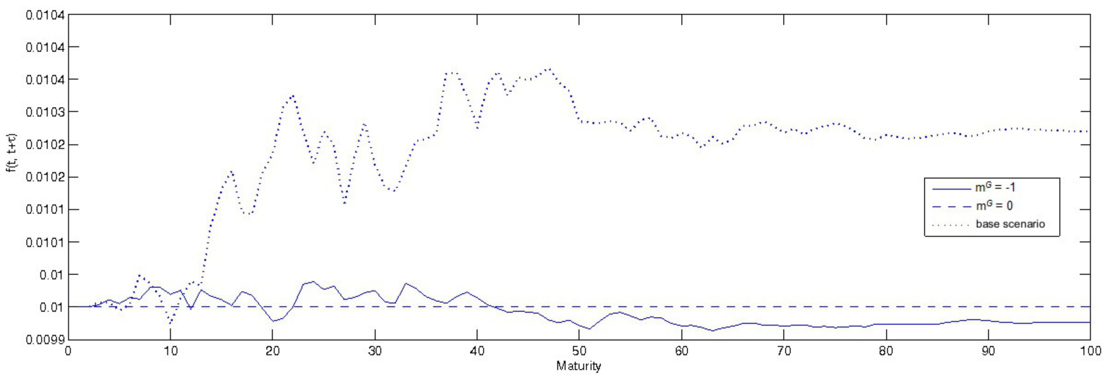
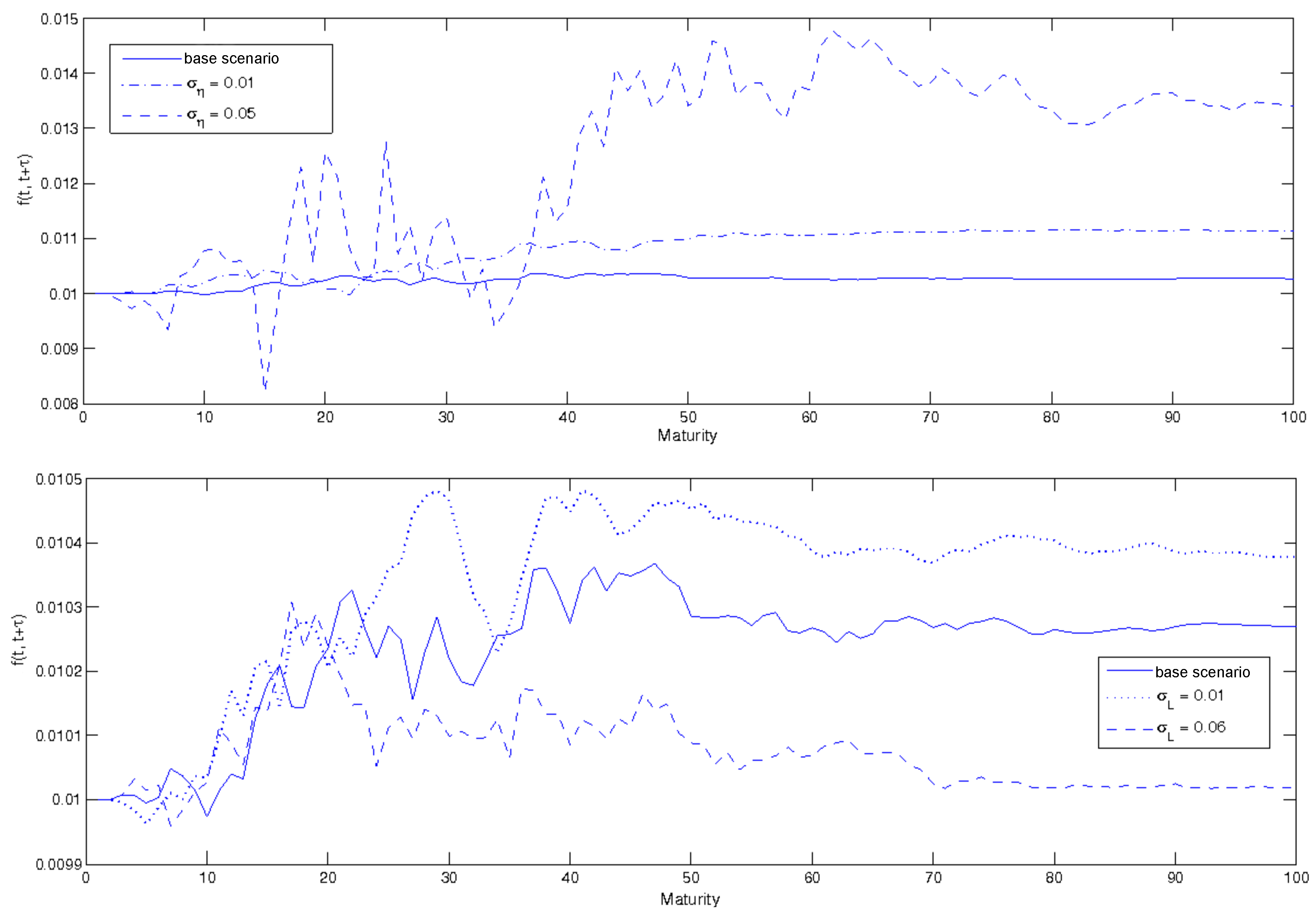
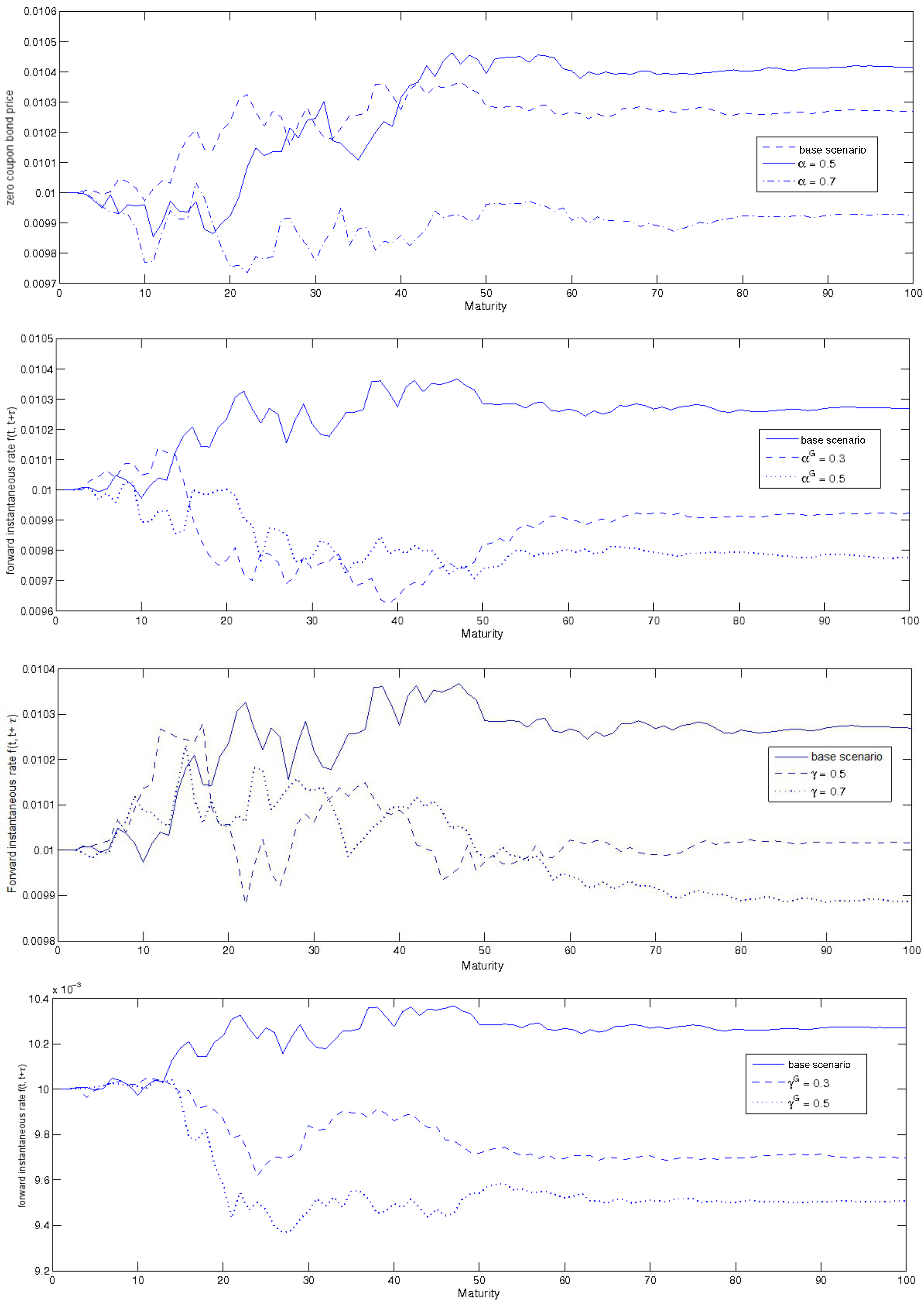
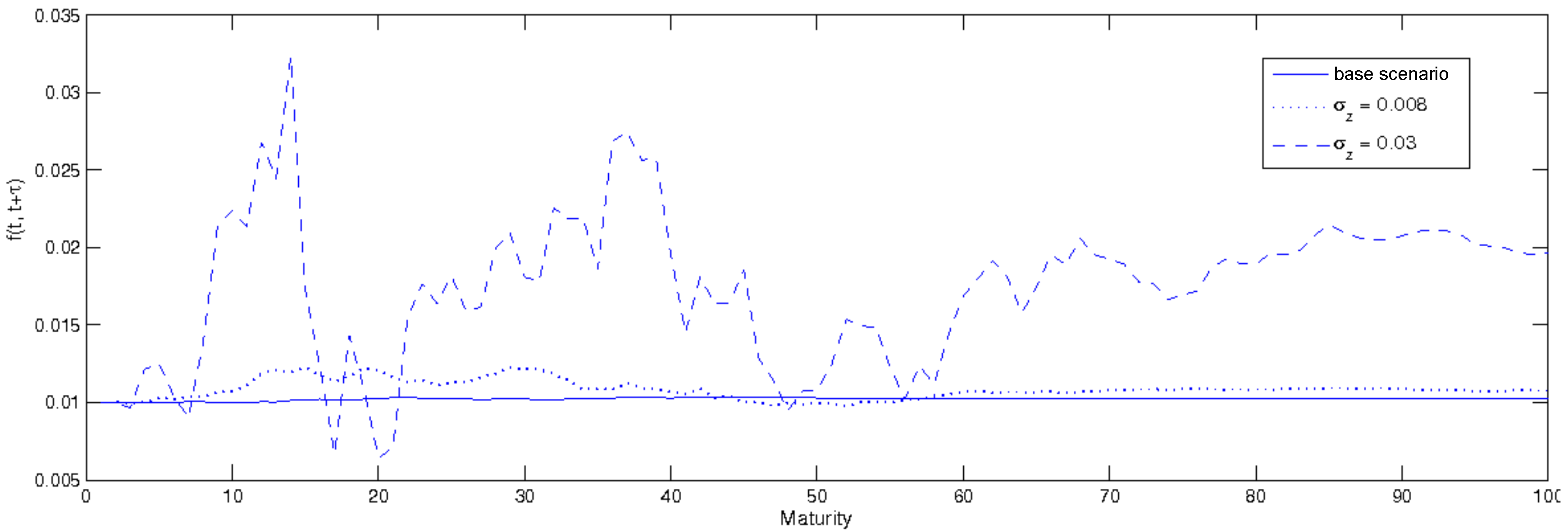
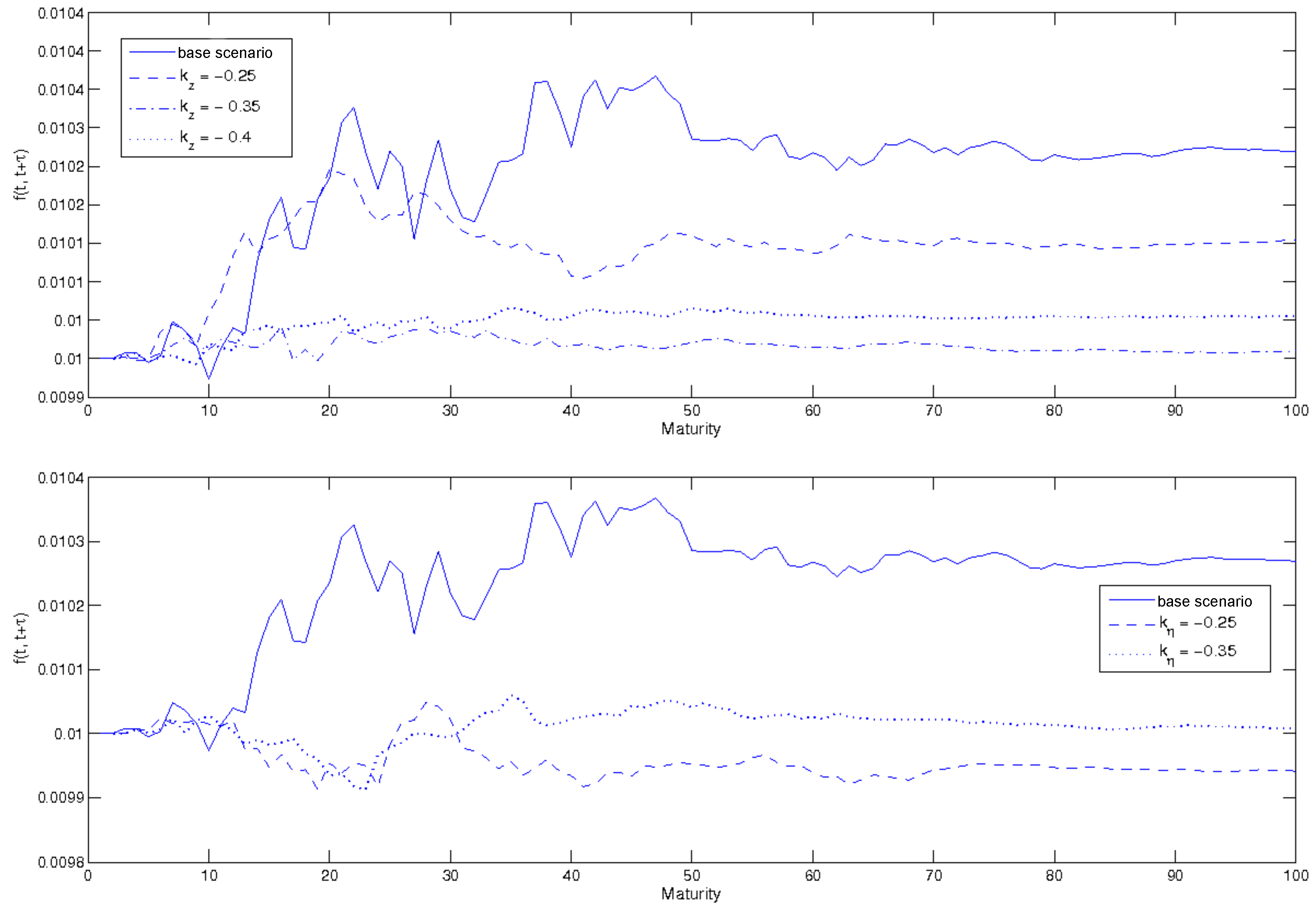
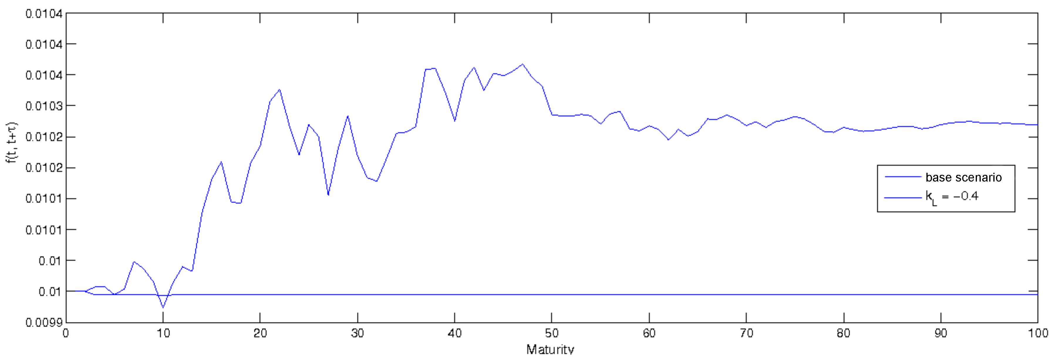
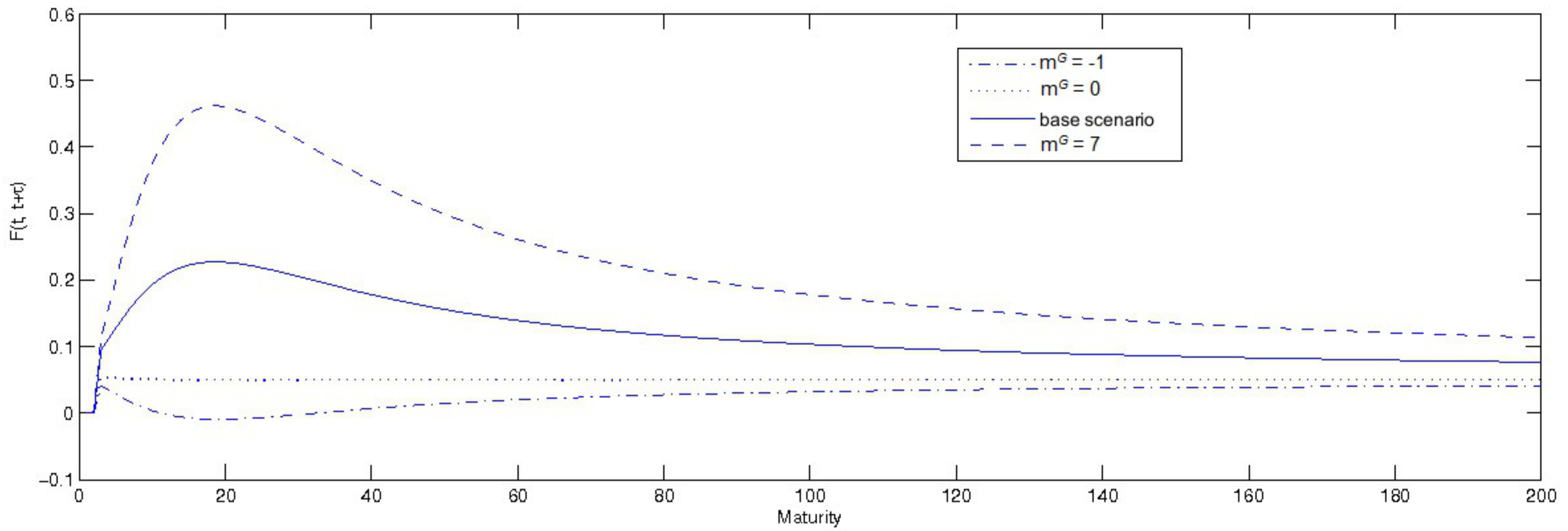
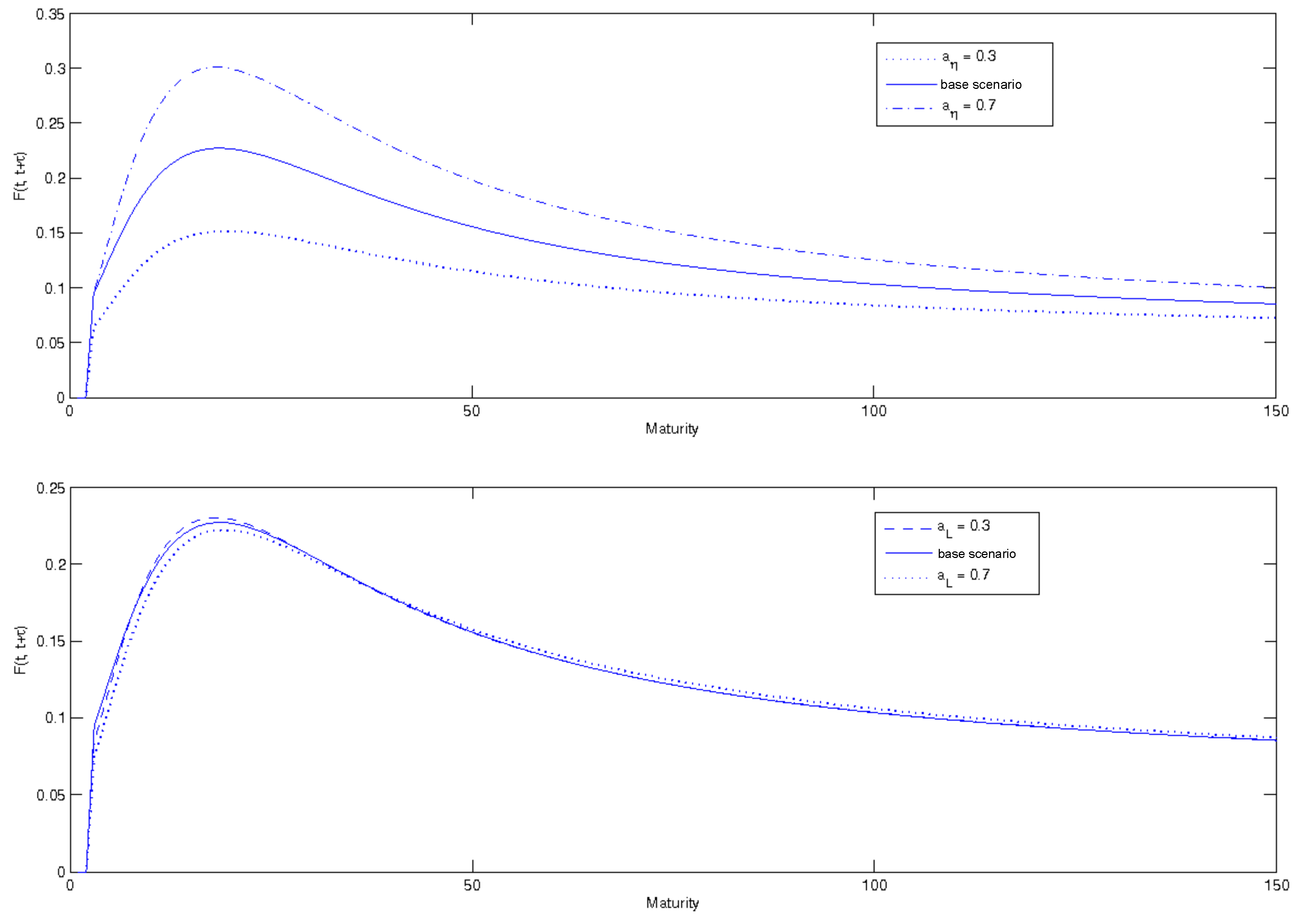
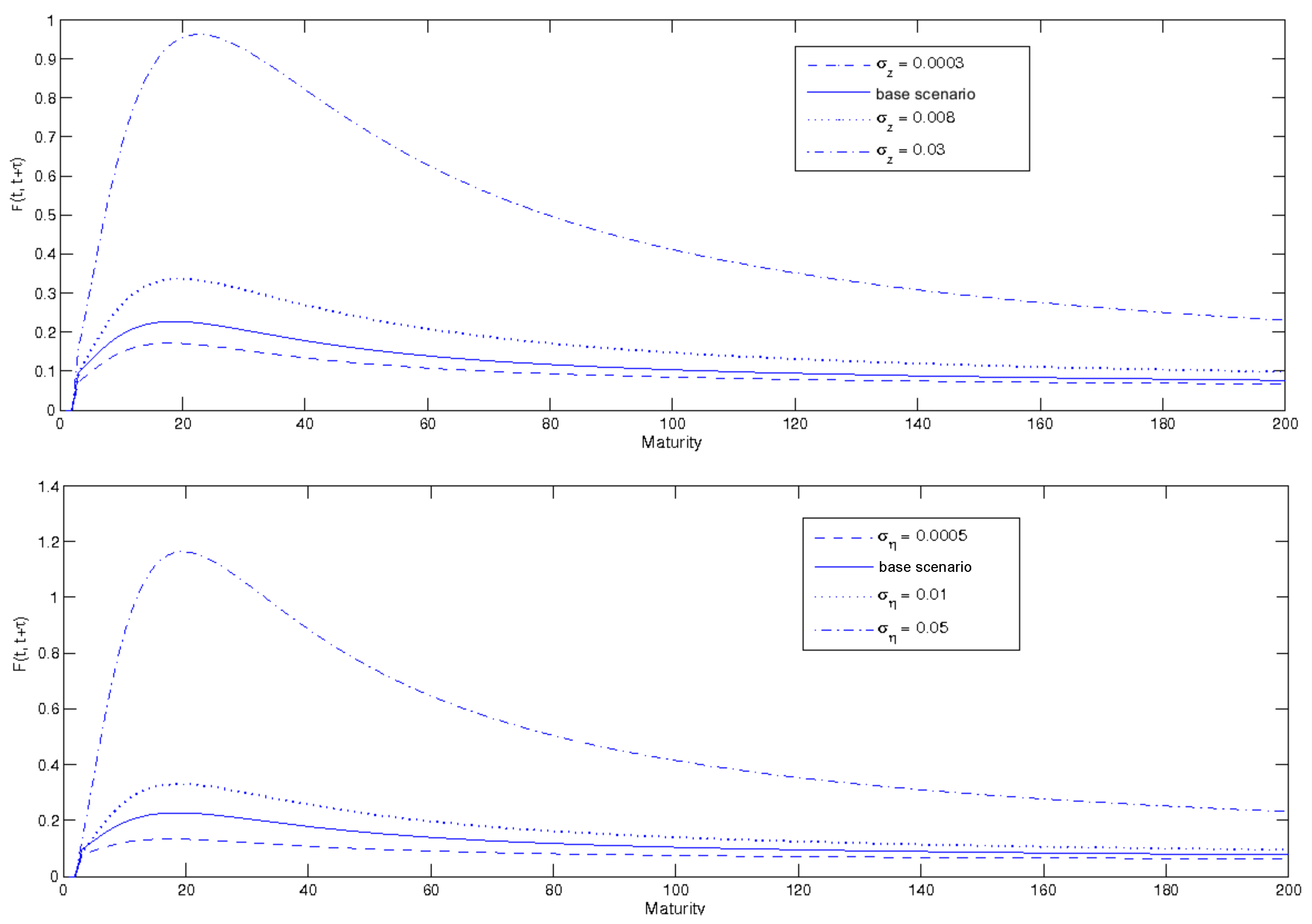
3.2.2. Forward Instantaneous Rate: A Sensitivity Analysis

Let us now move to a sensitivity analysis of the forward instantaneous rate with ambiguity, using different values of the parameters within f ( t , t + τ ) which allow us to focus on a more ambiguous scenario than the normal one. Regarding the baseline more ambiguous scenario, here we considered:
  • m G = 10;
  • zero correlation between Brownian motions;
  • both kinds of perceived ambiguity ( a η and a L ) are equal to 0.5 and 0.6, respectively;
  • volatilities set to σ z = 0.002 , σ η = 0.003 , σ L = 0.004 ;
  • the coefficients k z , k η , and k L have been set equal to −0.015, −0.03, −0.035.
As we are going to see, the following figures show the mean reverting feature of f ( t , t + τ ) : regardless of the shocks and the volatility, it tends toward its long-run trend level.
Figure 7 shows that the more government action minimizes the utility of the individuals, the lower the instantaneous forward rate. This result agrees with Figure 1, where the price path was complementary opposite to the one observed here (i.e., the volatility of the zero coupon bond price increased as the government acted maliciously). As a consequence, the forward instantaneous rate—derived substantially from the volatility of the price of the zero coupon bond—shows an opposite trend compared to the one seen for the price.
Other interesting analyses were conducted assuming different scenarios of correlation between the Brownian motions W t z ^ , W t G , h G , W t η , h η , W t L , relating to economic variables considered in this model. The baseline scenario examined in all the following charts corresponds to the case of normal ambiguity, related to m G = 3, and to the following assumptions:
  • correlation coefficients are all equal to zero;
  • the uncertainties perceived by the economic individuals ( a η and a L ) are equal to an average value (0.5);
  • the volatility parameters have been calibrated on low but realistic values: σ z = 0.003 , σ η = 0.005 , σ L = 0.006 ;
  • the coefficients k z , k η and k L have been calibrated on −0.15, −0.1, −0.05.
Observing the five graphs with correlated Brownian motions, we see that the higher the correlation, the lower the forward instantaneous rate. Moreover, in the case of correlated Brownian motions, the forward instantaneous rate tends to a lower trend level than the one reached in the baseline scenario (in which all the Brownians are independent).
For instance, the first graph from Figure 8 shows the forward instantaneous rate related to different correlation levels between W t z ^ and W t η , h η Brownian motions14. The same consideration reported above is also valid for the other three graphs reported in Figure 8. The second graph shows the forward instantaneous rate in scenarios of different correlation between W t G , h G and W t η , h η , the former representing the shock on consumption occurred under the distorted measure after government interventions, and the latter representing the known-unknown ambiguity. A positive (and different from zero) correlation15 α means that a positive shock W t z ^ corresponds to a positive shock on W t η , h η . In detail, this means that the economic growth and greater wealth resulting from shock W t z ^ will be associated with a greater known-unknown uncertainty. This is consistent with the economic model we are working with, as more consumption will lead individuals to believe that government action aims at consumption increase, different from the reference opinion. Given that a greater known-unknown uncertainty causes a higher zcb price, the forward instantaneous rate will decrease.
In Figure 8 (third and fourth graphs), we also compare forward instantaneous rates resulting from different correlation degrees between W t z ^ and W t L . In this case, the higher the γ , the lower the forward instantaneous rate. This occurs because the volatility will increase after a positive shock W t z ^ . Assuming a downward economic cycle phase (situation in which in reality the volatility increases), the uncertainty concerning the effectiveness of the policies implemented by the government will also increase. Another interesting point coming from correlation with unknown-unknown uncertainty is the clarity of the plunge of forward instantaneous rate. It seems that when investors doubt a government’s policy’s efficacy, that kind of shock immediately transfers as a shock on consumption and the economic cycle, and this effect is well-captured by our instantaneous rate.
In Figure 8, we notice the f ( t , t + τ ) rate decreasing to higher correlation between W t G , h G and W t L . This behavior is coherent with the assumptions of the economic model we are using; in fact, a greater uncertainty has a direct and positive effect on consumption (under the distorted opinion).
Finally, the chart in Figure 9 shows that a positive correlation between the two ambiguity sources W t η , h η and W t L leads to a decrease in the forward instantaneous rate and ultimately to an increase in the zcb price. The charts in Figure 10 seem to tell us that a greater uncertainty perceived by actors within the economy is reflected in lower zcb prices, and thus in higher forward instantaneous rates. Besides, Figure 11 gives us other information on the forward instantaneous rate coming from the zcb price path.
The charts in Figure 12 show opposite paths of the forward instantaneous rate f ( t , t + τ ) with increasing (absolute value) k parameters. This misleading behaviour is due—once again—to opposite effects summing up in one expression, i.e., the zcb price volatility. In more detail, the ambiguous effect of the k parameters help us to explain this unclear path.

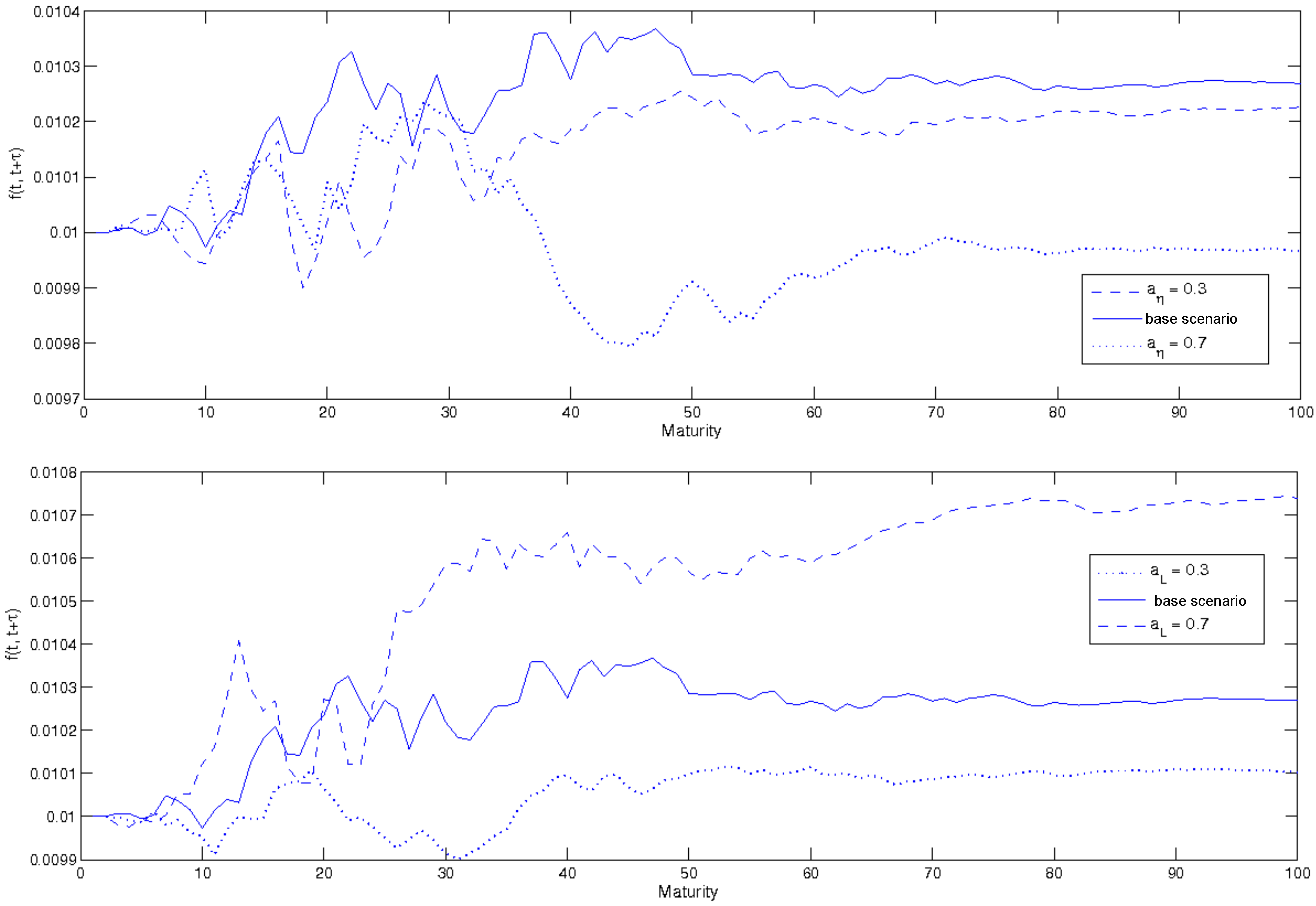
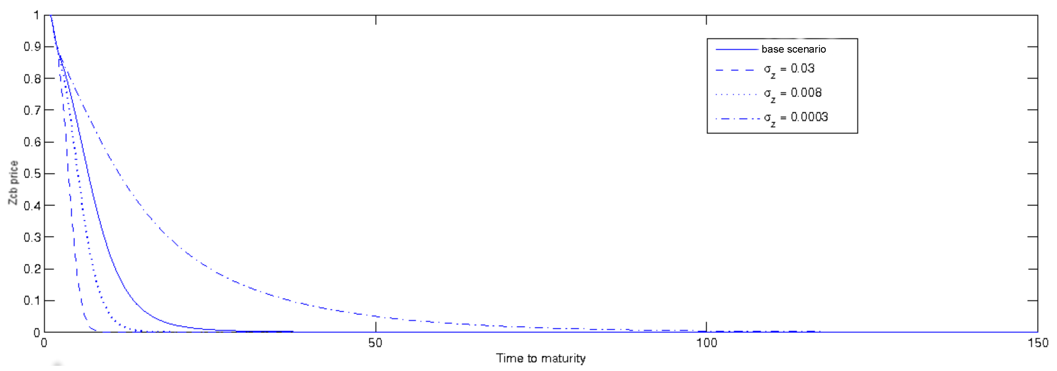
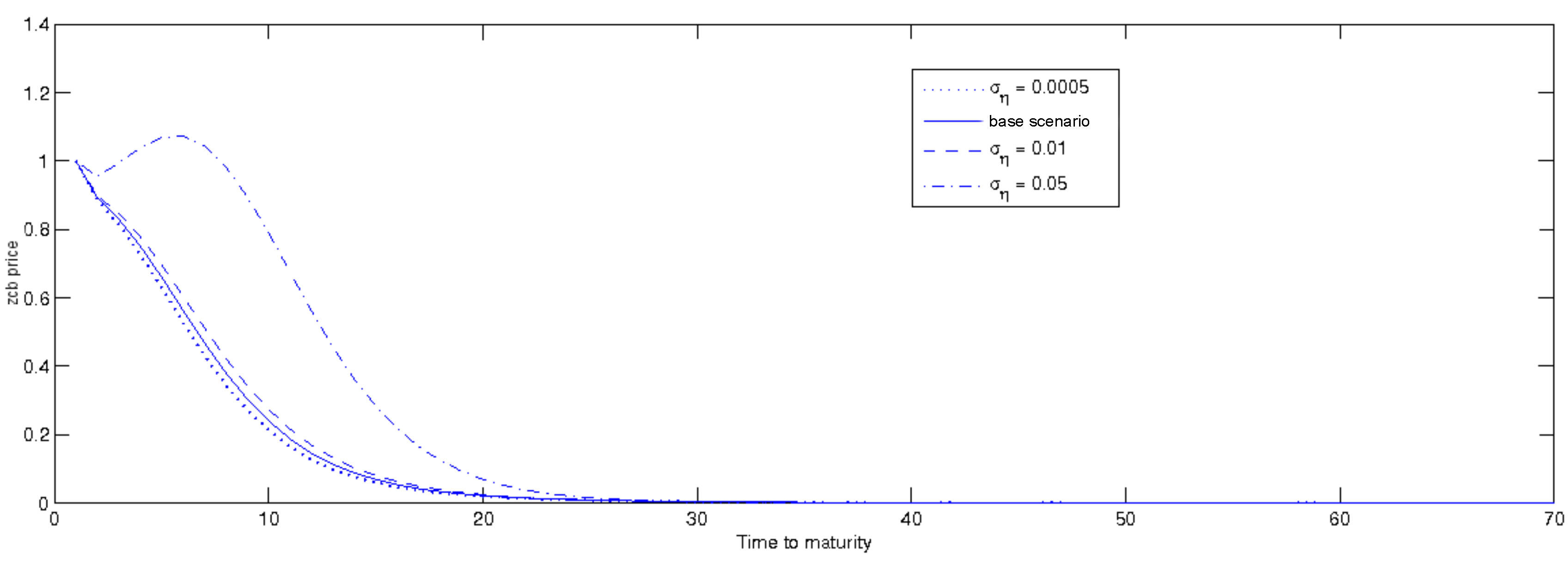
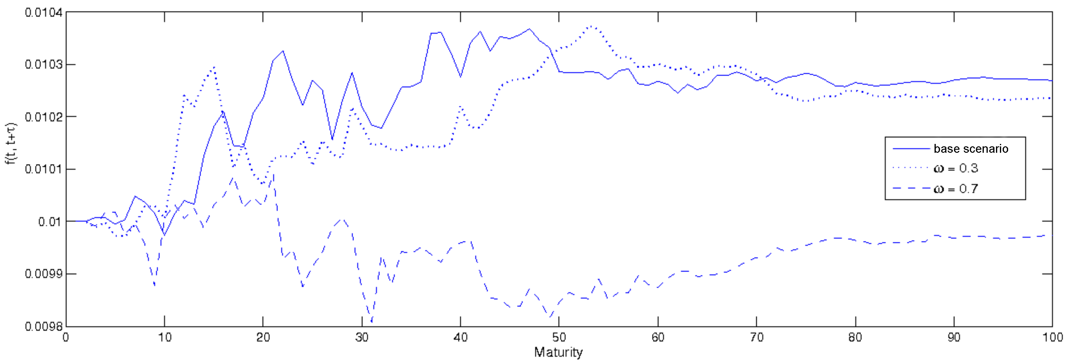
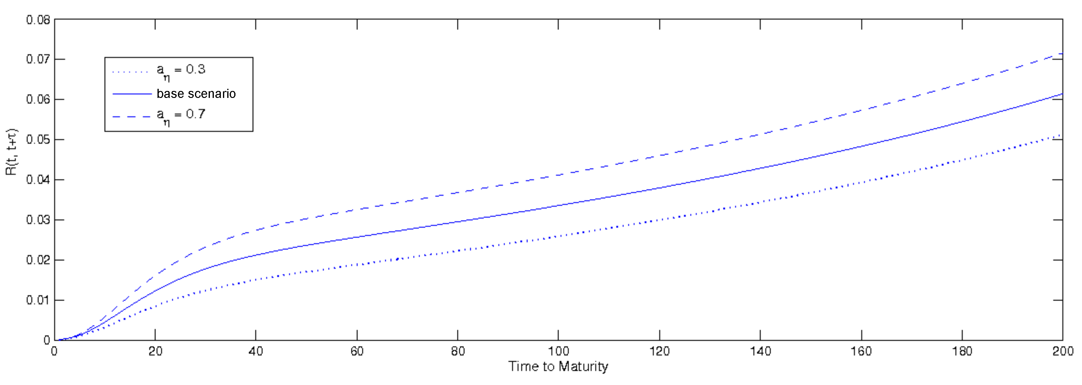
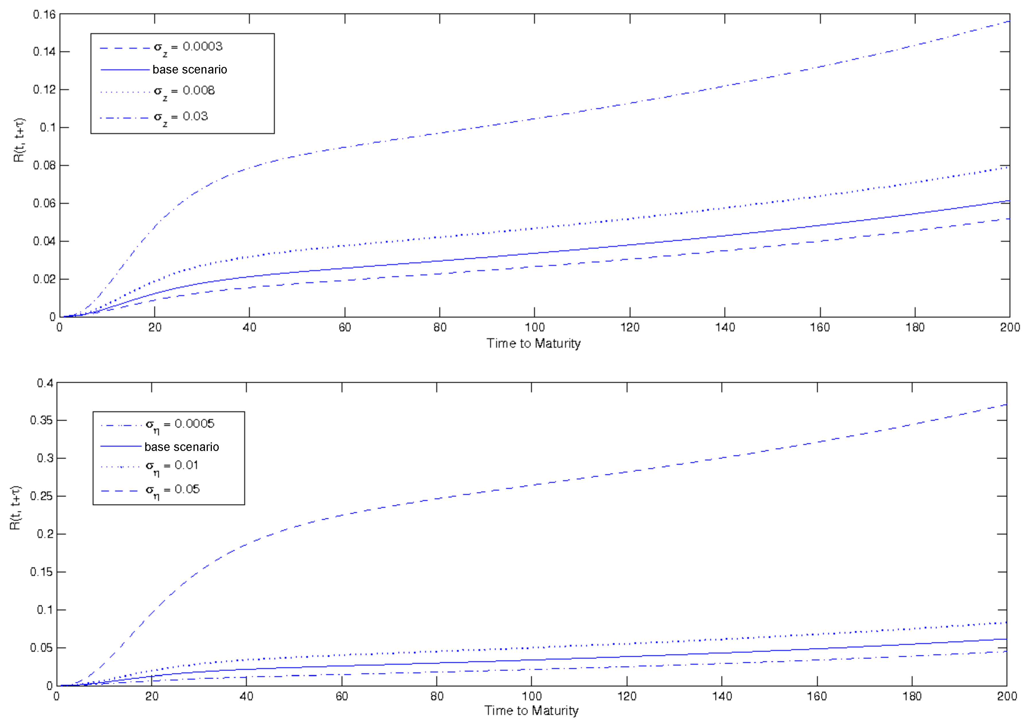
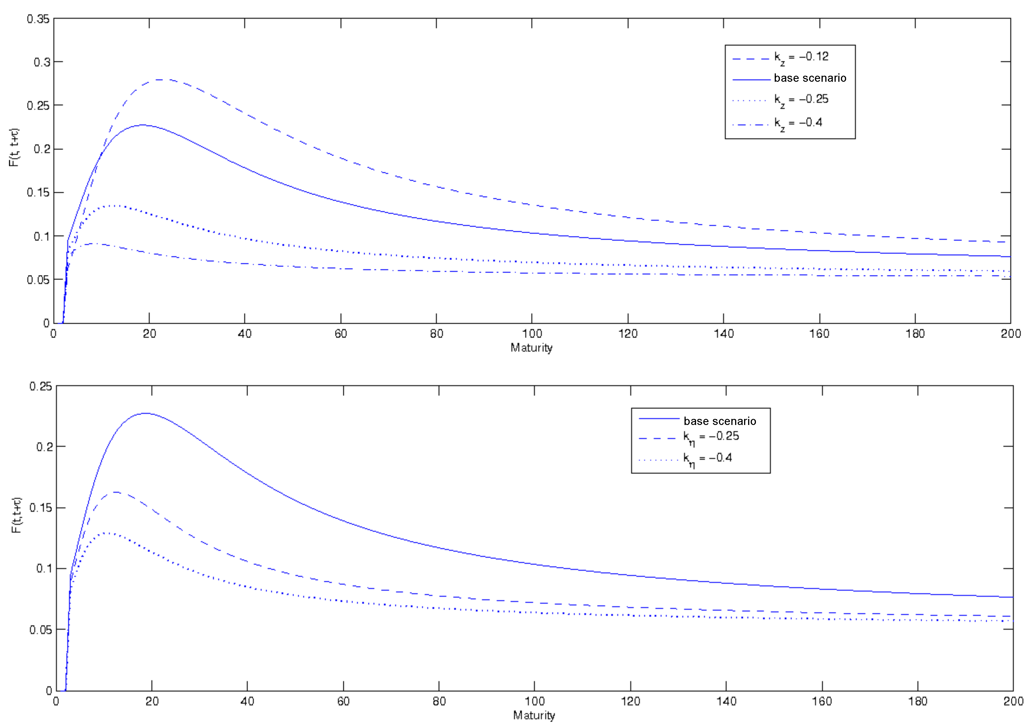
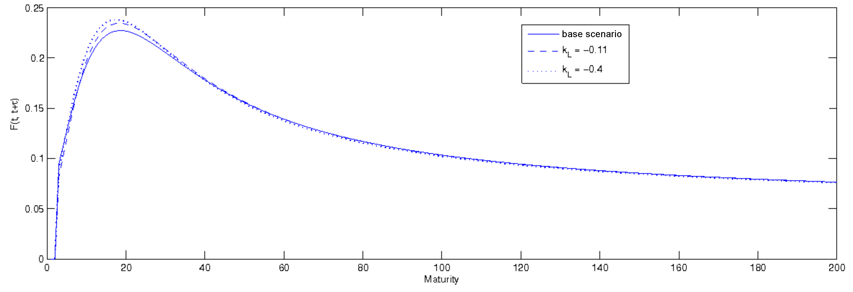
3.2.3. Spot and Forward Yields: A Sensitivity Analysis

This section analyses the behaviour of spot and forward rates implied in zero coupon bond prices with ambiguity. Our goal is to determine if and to what degree ambiguity factors may alter the usual spot yield curve.
The baseline scenario set out in the following figures—both spot and forward yield—uses these coefficients:
  • correlation coefficients are all equal to zero;
  • the number of policies available for government’s use ( m G ) is set to 3, which is linked to “normal” ambiguity scenario, as we saw earlier in this section;
  • the uncertainties perceived by the economic individuals ( a η and a L ) are equal to an average value (0.5);
  • the volatility parameters have been calibrated on low but realistic values: σ z = 0.003 , σ η = 0.005 , σ L = 0.006 ;
  • the coefficients k z , k η , and k L have been calibrated at −0.15, −0.1, −0.05.
Figure 13 shows a representation of how the rate holds its path even with a different number of policies available to the government. This finding confirms once again that short-term yield behaviour is opposite to the one of the zero coupon bond prices represented in (Figure 1).
Figure 14 shows a direct effect of the known-unknown uncertainty on the short yield: in fact, the greater the uncertainty the higher the rate, even considering a short-term yield. This sensitivity is suitable to explain what happened to Italian zero coupon bonds during sovereign debt crisis (2011–2012): within a few months, political instability created a climate of high uncertainty, which led to a strong increase in spot yields.
Regarding the ambiguity factors’ volatility16, our findings are slightly different. With regard to σ z , we find results which are consistent with our expectations: the greater the σ z , the lower the zcb price, and the higher the spot yield. A greater σ η instead leads to a higher spot yield, which at first would not have been an expected effect. However, if we go back to the spot yield expression with ambiguity, we will notice that the final effect is given by the term σ η k L . In this case, an increase in σ η determines an increase in spot yield because there is a dominance of the ambiguity over the other parameters, as also shown in Figure 15.
Figure 16 shows how the spot yield decreases if the three k parameters decrease (whereas the zcb price increases).
The following charts show the forward yield, where in order to simplify the sensitivity analysis, we put the trade date equal to zero and let delivery date and maturity date change. In other words, we led the analysis on B ( 0 , t , t + τ ) .
As for the spot yield, in the following charts we will observe a fully opposite behavior to the one of the zero coupon bond price, merely for the analytical form of the yield, found from the zero coupon bond price. For the forward yield we do not have a monotonous path; instead, we observe first an increase and then a decrease. This behavior tells us a great deal about the sensitivity to ambiguity. In fact, the longer the maturity of the government bond, the less information on the future, and so the more uncertainty. The expected effect of ambiguity is a rate increase, and for the previous considerations the importance of ambiguity effect becomes increasingly remarkable the longer the maturity, thus explaining the performance of the forward yield.
As we can see in Figure 17, the greater the number of available models that the government can choose from, the greater the forward yield (the opposite of what occurs for the zcb price). The same behaviour is observed in the case of an increase in the uncertainty perceived by economic individuals (Figure 18).
The path of the forward yield in the first chart in Figure 19 is coherent with the same sensitivity analysis led on the zcb, while the second chart follows the same explanation of Figure 15.
Finally, among the charts in Figure 20, the most interesting is the third, representing the sensitivity of the forward yield to the k L parameter, related with ambiguity source. Here, there is a strong dominance of the ambiguity on the other parameters, thus leading the represented trend.

4. Conclusions

Until 2007, the financial industry and economic theory based the majority of their work on the concept of risk. From 2007 on, the unpredicted and unpredictable events which took place in the world moved the attention to uncertainty, which is better suited to measuring situations which have not occurred before.
Uncertainty had been studied for years in the context of statistics and economic preferences by the foundational theory of ambiguity. This work extends the applicability of the ambiguity concept to help explain interest rate term structure, as we firmly believe that ambiguity is involved in the pricing process. As a matter of fact, the aim of this work is to provide an HJM framework which takes into account ambiguity in pricing process. In fact, political and economic events which occurred recently showed us many unpredicted situations which were difficult to understand (both quantitatively and qualitatively), and therefore out of the concept of risk, and much closer to the uncertainty (or ambiguity) concept.
In this way we built a model which could be useful both for pricing purposes and as a tool to better understand changes in economic indicators. Thanks to a sensitivity analysis, we monitored the effect that each parameter has on zero coupon bonds, spot, and forward (both yields and instantaneous) rates. Moreover, the discussion of a few main examples taken from reality also gave a grasp of how the model could help in explaining changes in GDP during periods of growing ambiguity.
Our research opens the way to future works about ambiguity, such as gauging the severity of ambiguity’s impact or studying the effects of long ambiguity periods on a country’s economy, exploring the effects of inflation in an economy pervaded by ambiguity, or exploring how different countries’ governments around the world can be classified on a scale of ambiguity.

Author Contributions

The authors shared the work out equally among themselves for that concerns both the theoretical and the empirical part of the contribution as well the writing.

Conflicts of Interest

The authors declare no conflict of interest.

References

  1. Cox, John C., Jonathan E. Ingersoll Jr., and Stephen A. Ross. 1985. A Theory of the Term Structure of Interest Rates. Econometrica 53: 385–408. [Google Scholar] [CrossRef]
  2. Duffie, Darrell, and Rui Kan. A yield-factor model of interest rates. Mathematical Finance 6: 379–406. [CrossRef]
  3. El Karoui, Nicole, and Vincente Lacoste. 1992. Multifactor Models of the Term Structure of Interest Rates. In AFFl Conference Proceedings. Paris: University of Paris. [Google Scholar]
  4. Ellsberg, Daniel. 1961. Risk, ambiguity and the Savage Axioms. The Quarterly Journal of Economics 75: 643–69. [Google Scholar] [CrossRef]
  5. Fox, Craig R., and Amos Tversky. 1995. Ambiguity aversion and comparative ignorance. The Quarterly Journal of Economics 110: 585–603. [Google Scholar] [CrossRef]
  6. Gagliardini, Patrick, Paolo Porchia, and Fabio Trojani. 2009. Ambiguity aversion and the term structure of interest rates. Review of Financial Studies 22: 4157–88. [Google Scholar] [CrossRef]
  7. Ghirardato, Paolo, Fabio Maccheroni, and Massimo Marinacci. 2004. Differentiating ambiguity and ambiguity attitude. Journal of Economic Theory 118: 133–73. [Google Scholar] [CrossRef]
  8. Gilboa, Itzhak, and David Schmeidler. 1989. Maxmin Expected Utility with non unique prior. Journal of Mathematical Economics 18: 141–53. [Google Scholar] [CrossRef]
  9. Hansen, Lars Peter, and Thomas J. Sargent. 2008. Robustness. Princeton: Princeton University Press. [Google Scholar]
  10. Heath, David, Robert Jarrow, and Andrew Morton. 1992. Bond Pricing and the Term Structure of Interest Rates: A New Methodology for Contingent Claims Valuation. Econometrica 60: 77–105. [Google Scholar] [CrossRef]
  11. Ho, Thomas SY, and Sang-Bin Lee. 1986. Term Structure Movements and Pricing Interest Rate Contingent Claims. Journal of Finance 41: 1011–29. [Google Scholar] [CrossRef]
  12. Ilut, Cosmin L., and Martin Schneider. 2014. Ambiguous business cycles. The American Economic Review 104: 2368–99. [Google Scholar] [CrossRef]
  13. Kast, Robert, André Lapied, and David Roubaud. 2014. Modelling under ambiguity with dinamically consistent Choquet random walks and Choquet-Brownian motions. Econ Modell 38: 495–503. [Google Scholar] [CrossRef]
  14. Knight, Frank H. 1921. Risk, Uncertainty, and Profit. Boston: Houghton Mifflin. [Google Scholar]
  15. Musiela, Mark. 1994. Nominal Annual Rates and Lognormal Volatility Structure. Working paper, The University of New South Wales, Sydney, Australia. [Google Scholar]
  16. Savage, Leonard J. 1954. The Foundations of Statistics. New York: Wiley. [Google Scholar]
  17. Schmeidler, David. 1989. Subjective probability and expected utility without additivity. Econometrica 57: 517–87. [Google Scholar] [CrossRef]
  18. Ulrich, Maxim. 2008. Inflation Ambiguity and the Term Structure of Arbitrage Free US Government Bonds. New York: Columbia University. [Google Scholar]
  19. Ulrich, Maxim. 2011. How Does the Bond Market Perceive Government Interventions? WFA 2011, NBER Asset Pricing. New York: Columbia Business School. [Google Scholar]
  20. Vasicek, Oldrich. 1997. An Equilibrium Characterization of the Term Structure. Journal of Financial Economics 5: 177–88. [Google Scholar] [CrossRef]
1
As a matter of fact, Ulrich (2011) reports that the uncertainty about government interventions and multiplier uncertainty are able to predict annual bond premium of bonds with R 2 of 25% and 14%.
2
A capacity is a function which on a set (S, Σ ) is monotonous and normalized. Moreover, a capacity becomes a probability measure if it is finitely additive. On the other side, the Choquet integral was set up to work with capacities.
3
We restrict the model to the affine structure of the factors which are affine on a single factor (i.e., the instantaneous interest rate). In this way, we work in line with Duffie and Kan (1996) and El Karoui and Lacoste (1992), where the dynamic of the factors—which are interest rates for several maturities—is chosen in order to ensure the absence of arbitrage assumption. The famous Vasicek (1997), Cox et al. (1985) models for the factors are both coherent with this assumption because they lead to an affine structure of the factors on the instantaneous interest rate.
4
In the case of an n-dimensional Brownian motion with independent component, the completeness condition is n d ; in the dependent case, we must include the covariances in the computation of the sources of risk.
5
In line with the previous modeling, the ambiguous version of a one-dimensional exponential-affine model will be a two-factor model in order to include the ambiguity as an exogenous factor. On the other hand, if the single factor is modeled in terms of a Choquet–Brownian, as suggested in Kast et al. (2014), we would be able to endogenously introduce the ambiguity, preserving the original dimension of the factors’ set.
6
If Ricardian equivalence is true, this component is zero.
7
This set is defined in order to have a relative entropy between a non-zero multiplier policy and a zero-multiplier policy which is bounded from above by a positive but small number; i.e., k t = A η t 2 , variable in time. Hence, the complexity of H is variable in time as well as the agent’s uncertainty.
8
A max-max agent aims to invest into a robust portfolio; i.e., paying off well if government was indeed implementing first-best policies not corresponding to the benchmark (zero-multiplier policy).
9
For this reason, we can see the dynamic of η t as an approximation of a squared root process.
10
For this reason we can see the dynamic of L t as an approximation of a squared root process.
11
We use c 0 (i.e., the sample mean of quarterly GDP growth) to demean the median forecast.
12
The case of post-election in France was not examined due to a lack of data.
13
The analysis led on the parameter k L has been omitted due to the absence of relevant results.
14
W t z ^ represents the stochastic part inside economic cycle, meaning with this the technological progress achieved in the economy, while W t η , h η represents the known-unknown ambiguity.
15
We did not consider cases with negative correlation, as they would have been incoherent with the economic model underlying the Ulrich (2011) model.
16
σ L has been omitted because of the lack of sensitivity in the analysis.
Figure 1. Zero coupon bond price in different government action hypotheses .
Risks 05 00050 g001
Figure 2. Zero coupon bond price based on different ambiguity levels.
Risks 05 00050 g002
Figure 3. Zero coupon bond price in different hypothesis of economic cycle volatility.
Risks 05 00050 g003
Figure 4. Zero coupon bond price in different hypothesis of known-unknown uncertainty volatility.
Risks 05 00050 g004
Figure 5. Zero coupon bond price in different hypothetical levels of k z .
Risks 05 00050 g005
Figure 6. Zero coupon bond price in different hypothetical levels of k η .
Risks 05 00050 g006
Figure 7. Performance of the instantaneous forward rate to various government actions.
Risks 05 00050 g007
Figure 8. Forward instantaneous rate for various levels of correlation coefficients α , α ¯ , γ , γ ¯ .
Risks 05 00050 g008
Figure 9. Forward instantaneous rate for various levels of correlation coefficient ω .
Risks 05 00050 g009
Figure 10. Forward instantaneous rate to varying ambiguity perceived by the economic individuals.
Risks 05 00050 g010
Figure 11. Forward instantaneous rate to varying volatility of ambiguity factor L.
Risks 05 00050 g011aRisks 05 00050 g011b
Figure 12. Forward instantaneous rate to varying parameters k z , k η , and k L .
Risks 05 00050 g012aRisks 05 00050 g012b
Figure 13. Short yield to different government policies.
Risks 05 00050 g013
Figure 14. Short yield to various degrees of known-unknown uncertainty.
Risks 05 00050 g014
Figure 15. Spot yield to varying parameters σ z and σ η .
Risks 05 00050 g015
Figure 16. Spot yield to varying parameters k z , k η , and k L .
Risks 05 00050 g016
Figure 17. Forward yield in different scenarios of government actions.
Risks 05 00050 g017
Figure 18. Forward yield for different degrees of uncertainty perceived by economic individuals.
Risks 05 00050 g018
Figure 19. Forward yield for different volatilities σ z and σ η .
Risks 05 00050 g019
Figure 20. Forward yield when parameters k z , k η , and k L change.
Risks 05 00050 g020aRisks 05 00050 g020b
Table 1. Empirical evaluation of the impact of ambiguity: some examples.
m G a η
Pre-Brexit1.866480.2
Post-Brexit2.357660.2
Pre-referendum Italy4.4270.1
Post-referendum Italy2.76730.2
Pre-election France6.230520.1

