Assessment of Policy Changes to Means-Tested Age Pension Using the Expected Utility Model: Implication for Decisions in Retirement

Abstract

Means-tested pension policies are typical for many countries, and the assessment of policy changes is critical for policy makers. In this paper, we consider the Australian means-tested Age Pension. In 2015, two important changes were made to the popular Allocated Pension accounts: the income means-test is now based on deemed income rather than account withdrawals, and the income-test deduction no longer applies. We examine the implications of the new changes in regard to optimal decisions for consumption, investment and housing. We account for regulatory minimum withdrawal rules that are imposed by regulations on Allocated Pension accounts, as well as the 2017 asset-test rebalancing. The policy changes are considered under a utility-maximising life cycle model solved as an optimal stochastic control problem. We find that the new rules decrease the advantages of planning the consumption in relation to the means-test, while risky asset allocation becomes more sensitive to the asset-test. The difference in optimal drawdown between the old and new policy is only noticeable early in retirement until regulatory minimum withdrawal rates are enforced. However, the amount of extra Age Pension received by many households is now significantly higher due to the new deeming income rules, which benefit wealthier households who previously would not have received Age Pension due to the income-test and minimum withdrawals.

1. Introduction

Means-tested pension policies become more important globally, as the general population ages and the life expectancy improves. The policies are country-specific to meet government budgets and are updated regularly. Since the Australian retirement system is relatively young, the long-term effects of this new pension system are not yet known. Changes to policy, means-tests and tax rules are expected to occur frequently due to fiscal reasons and once the effects of policy changes to a retiree’s personal wealth (and the economy in general) become evident. Variables directly related to the means-test such as entitlement age, means-test thresholds, taper rates and pension payments can all be adjusted to meet budget needs by the government. On a larger scale, regulatory changes may include whether the family home is included in the means-tested assets, the elimination of minimum withdrawal1 rules, changes in mandatory savings rates or additional taxes on superannuation savings. From a mathematical modelling perspective, this poses difficulties in terms of future model validity, as regulatory risk and policy changes can quickly make a model obsolete if it is not modified to account for the new rules.

The Australian pension system is based on the compulsory superannuation2 guarantee (paid by employers), private savings, and a government-provided means-tested Age Pension. The superannuation guarantee, supporting both defined-benefit and defined-contribution pension plans, mandates that employers contribute a fixed percentage of the employee’s gross earnings to a superannuation fund, which accumulates and is invested until retirement. The current contribution rate is set to 9.5%, and additional contributions attract certain tax benefits. Private savings are comprised of these additional contributions, but also include savings outside the superannuation fund such as investment accounts, dwelling and other assets. Finally, the Age Pension is a government-managed safety net, which provides the retiree with a means-tested Age Pension. This means-test determines whether the retiree qualifies for full, partial or no Age Pension once the entitlement age is reached. In this means-test, income and assets are evaluated individually, and a certain taper rate reduces the maximum payments once income or assets surpass certain thresholds (which are subject to family status and home-ownership). Income from different sources is also treated differently; financial assets are expected to generate income at the so-called deeming rate, while income streams such as labour and annuity payments that are not from a pension account are assessed based on their nominal value.

The motivation for this paper was the recent changes for Allocated Pension accounts, where assets are now assumed to generate a deemed income and no longer have an income-test deduction. Account-based pensions (such as Allocated Pension accounts) are accounts that have been purchased with superannuation and generate an income stream throughout retirement. Such an account does not have tax on investment earnings and is subject to regulatory minimum withdrawal rates each year, which increase with age. Prior to 2015, these types of accounts allowed for an income-test deduction that was determined upon account opening, and withdrawals were considered to be income in the means-test. The income-test deduction allowed the retiree to withdraw slightly more every year without missing out on Age Pension. However, in 2015, the rules changed. Existing accounts were ‘grandfathered’ and will continue to be assessed under the old rules, while the new rules will be applied to any new accounts. The arguments for the changes were simplicity (people with the same level of assets should be treated the same, regardless of how the assets are invested), to increase incentive to maximise total disposable income rather than maximising Age Pension payments and to simplify how capital growth and interest-paying investments are assessed (Department of Social Services 2017). From a fiscal point of view, the recommendation to introduce the new rules was based on estimated unchanged costs3 (Henry 2009); however, the 2015–2016 budget stated expected savings of $57 million for 2015–2016 and $129 million and $136 million for subsequent years (The Commonwealth of Australia 2015). The allocation to Age Pension in the 2015–2016 budget includes all changes to the Age Pension in a combined viewpoint, so the specific impact of the deeming rule changes on the government is not known.

Problems with decisions that span over multiple time periods are typically modelled with life cycle models and solved with backwards recursion (Cocco et al. 2005; Cocco and Gomes 2012; Blake et al. 2014, to name a few). Life cycle modelling based on utility theory originates from Fisher (1930) and was later updated by Modigliani and Brumberg (1954), who observed that individuals make consumption decisions based on resources available at the current time, as well as over the course of their lifetimes. The key work for early models was laid out by Yaari (1964, 1965), who extended the model with uncertain lifetime and studied the optimal choice of life insurance and annuities, while Samuelson (1969) and Merton (1969, 1971) studied the problem in relation to optimal portfolio allocation. Nowadays, there are extended theories available such as prospect theory (Kahneman and Tversky 1979) or stochastic dominance theory (Kopa et al. 2016; Levy 2006). While prospect theory is based on the findings that individuals often violate expected utility maximization, the stochastic dominance is developed on the foundation of the expected utility paradigm. There is a plethora of research on retirement modelling internationally (Boender et al. 1997; Dupačová and Polívka 2009; Hilli et al. 2007; Vitali et al. 2017, to name a few), but there is still rather limited research modelling the Australian Age Pension, and even less that enforces the minimum withdrawal rules. The model in Ding (2014) does not constrain drawdown with minimum withdrawal, which would limit the author from finding a semi-closed form solution. Similarly, other authors that focus on means-tested pension also do not enforce minimum withdrawal rates, such as Hulley et al. (2013), who use Constant Relative Risk Aversion (CRRA) utility to understand consumption and investment behaviour, or Iskhakov et al. (2015), who investigate how annuity purchases change in relation to Age Pension. It should be noted that their assumptions do not include Allocated Pension accounts; thus, minimum withdrawal rates may not apply. However, as the majority of Australian retirees own an Allocated Pension account (or similar phased withdrawal products), there is surprisingly limited research conducted on the implications of the regulatory minimum withdrawal rates (Andreasson et al. 2017). The exception is Bateman et al. (2007), who compare the welfare of retirees when the current minimum withdrawal rates were introduced in 2007 against the previous rules and alternative drawdown strategies. The authors use a rather simple CRRA model to examine the effect of different risk aversion and investment strategies, but find that the minimum withdrawal rules increase the welfare for retirees, though slightly less than optimal drawdown does. In Andreasson et al. (2017), the minimum withdrawal rules are included in part of the model outcome, but are by no means exhaustive and only provide a brief introduction to the effects. These rules are designed to exhaust the retiree’s account around Year 100; however, it is empirically observed that after Year 85 (subject to investment returns), the withdrawn dollar amount starts decreasing quickly. In a recent report from Plan For Life (2016), it is identified that only 5% of retirees exhaust their accounts completely, though this number is expected to increase as life expectancy increases and the population ages. They find that retirees tend to follow the minimum withdrawal rules as guidelines for their own withdrawal, as few withdraw more than the minimum amount. This is further confirmed in Shevchenko (2016). However, Rice Warner (2015) argues that the minimum withdrawal rates should be cut by 25–50% to prevent retirees from exhausting their superannuation prematurely due to increased longevity. They suggest that the current rates are simply too high for many retirees, thus not sustainable for people living longer than the average life expectancy, and are significantly higher than what is optimal in Andreasson et al. (2017). In addition, it has been discussed in the media whether deeming rates are set too high, and as retirees tend to have a low proportion of risky assets while in retirement (Spicer et al. 2016), this often results in lower returns on assets than what is assumed in the income-test. The Australian term rates4 are below the upper deeming rate; hence, the effective return on the portfolio is generally lower than the deeming rate. This, in turn, will affect the Age Pension payments for the retiree.

In this paper, we demonstrate how the assessment of policy changes can be done via an expected utility model in the Australian pension system. We adapt the model previously developed in Andreasson et al. (2017) to examine the impact of this policy change on an individual retiree. This model captures retirement behaviour in the decumulation phase of Australian retirees subject to consumption, housing, investment, bequest and government-provided means-tested Age Pension and is an extension with stochastic factors (mortality, risky investments and sequential family status) to what was originally presented in Ding (2014); Ding et al. (2014). The contribution of this paper is to improve the understanding of the effect deeming rate-based policies have on a typical retiree’s optimal decisions, both in terms of how the optimal behaviour changes and whether the retiree is better or worse off. We also examine the impact high and low risky returns have on the retiree in relation to deeming rates. We then examine the differences in optimal decisions between an Allocated Pension account opened prior to 2015 with the one opened after 2015, as well as compare the results with the recent 2017 asset-test adjustments. The paper is structured as follows: In Section 2, we summarise the model and present the Age Pension function, as well as explain the parameterization and policies. Section 3 contains a discussion of the results. Finally, in Section 4, we present our concluding remarks.

2. Model

We begin with the setup of the utility model framework for the retirement phase. We adopt the model from Andreasson et al. (2017), where the Age Pension function has been adjusted to account for the policy changes in 2015. For a complete description of the model, its calibration to the data and numerical solution and a discussion of the construction and assumptions, please see that reference.

The objective of the retiree is to maximise expected utility generated from consumption, housing and bequest. The retiree starts off with a total wealth $\mathsf{W}$ and, at the year of retirement $t=t_0$, is given the option to allocate wealth into housing H (if he/she is already a homeowner, he/she has the option to adjust current allocation by up- or down-sizing). The remaining (liquid) wealth $W_{t_0}=\mathsf{W}-H$ is placed in an Allocated Pension account, which is a special type of account that does not have a tax on investment earnings and is subject to the regulatory minimum withdrawal rates. A retiree can either start as a couple or single household, where this information is contained in a family status random variable:

$$G_t\in \mathcal{G}=\{\Delta ,0,1,2\},$$

(1)

where $\Delta$ corresponds to the agent already deceased at time t, 0 corresponds to the agent who died during $(t-1,t]$ and 1 and 2 correspond to the agent being alive at time t in a single or couple household, respectively. Evolution in time of the family state variable $G_t$ is subject to survival probabilities. In the case of a couple household, there is a risk each time period that one of the spouses passes away, in which case, it is treated as a single household model for the remaining years.

At the start of each year $t=t_0,t_0+1,\dots ,T-1$, the retiree will receive a means-tested Age Pension $P_t$ and will decide what amount of saved liquid wealth $W_t$ will be used for consumption (defined as proportion drawdown ${\alpha }_t$ of liquid wealth). Consumption each period equals received Age Pension and drawdowns:

$$C_t=P_t+{\alpha }_t{W}_t.$$

(2)

Any remaining liquid wealth after drawdown can be invested in a risky or a risk-free asset, where ${\delta }_t$ determines the proportion invested in the risky asset. Then, the change in wealth after the decision to the next period is given by:

$$W_{t+1}=\left[W_t-{\alpha }_t{W}_t\right]\left[{\delta }_t{e}^{Z_{t+1}}+(1-{\delta }_t)e^{r_t}\right],$$

(3)

where $Z_{t+1}$ is the stochastic return on risky assets modelled as independent and identically distributed random variables from a normal distribution $\mathcal{N}(\mu ,\sigma )$ with mean $\mu$ defined in real5 terms and variance ${\sigma }^2$. Any wealth not allocated to risky assets is assumed to generate a deterministic real risk-free return $r_t$ (risk-free interest rate adjusted for inflation). Each period the agent receives utility based on the current state of family status $G_t$:

$$R_t(W_t,G_t,{\alpha }_t,H)=\left\{\begin{array}{cc}{U}_C(C_t,G_t,t)+U_H(H,G_t),\hfill & \mathrm{if} G_t=1,2,\hfill \\ U_B(W_t,H),\hfill & \mathrm{if} G_t=0,\hfill \\ 0,\hfill & \mathrm{if} G_t=\Delta .\hfill \end{array}\right.$$

(4)

That is, if the agent is alive, he/she receives reward (utility) based on consumption $U_C$ and housing $U_H$, if he/she died during the year, the reward comes from the bequest $U_B$, and if he/she is dead, there is no reward. Note that the reward received when the agent is alive depends on whether the family state is a couple or single household due to different utility parameters and Age Pension thresholds.

Finally, $t=T$ is the maximum age of the agent beyond which survival is deemed impossible, and the terminal reward function is given as:

$$\tilde{R}(W_T,G_T,H)=\left\{\begin{array}{cc}{U}_B(W_T,H),\hfill & \mathrm{if} G_T\ge 0,\hfill \\ 0,\hfill & \mathrm{if} G_T=\Delta .\hfill \end{array}\right.$$

(5)

The retiree has to find the decisions that maximise expected utility with respect to the decisions for consumption, investment and housing. This is defined as a stochastic control problem, where decisions (controls) at time t depend on the realisation of stochastic state variables $W_t$ and $G_t$ at time t with unknown future realisations. Then, the overall problem of maximization of expected utility is defined as:

$$\underset{H}{max}\left[\underset{\alpha ,\delta }{sup}{\mathbb{E}}_{t_0}^{\alpha ,\delta }\left[{\beta }_{t_0,T}\tilde{R}(W_T,G_T,H)+\sum _{t=t_0}^{T-1}{\beta }_{t_0,t}{R}_t(W_t,G_t,{\alpha }_t,H)|W_{t_0},G_{t_0}\right]\right],$$

(6)

where ${\mathbb{E}}_{t_0}^{\alpha ,\delta }[·]$ is the expectation with respect to the state variables $W_t$ and $G_t$ for $t=t_0+1,\dots ,T$, conditional on the state variables at time $t=t_0$ if we use controls $\mathit{\alpha }=({\alpha }_{t_0},{\alpha }_{t_0+1},\dots ,{\alpha }_{T-1})$ and $\mathit{\delta }=({\delta }_{t_0},{\delta }_{t_0+1},\dots ,{\delta }_{T-1})$ for $t=t_0,t_0+1,\dots ,T-1$. The subjective discount rate ${\beta }_{t,t^{\prime }}$ is a proxy for personal impatience between time t and $t^{\prime }$. Note that the death probabilities are not explicit in the objective function, but affect the evolution of the family status and, thus, are involved in the calculation of the conditional expectation. This problem can be solved numerically with dynamic programming by using backwards induction of the Bellman equation. The state variables W and H are discretized on a grid, and the Gaussian quadrature method is used for integration between periods; for details, see Andreasson et al. (2017).

2.1. Utility Functions

Utility in the model is measured with time-separable additive functions based on the commonly-used Hyperbolic Absolute Risk Aversion (HARA) utility function, subject to different utility parameters for singles and couples, as follows.

• Consumption preferences: It is assumed that utility comes from consumption exceeding the consumption floor, weighted with a time-dependent “health” status proxy6. The utility function for consumption is defined as:

  $$U_C(C_t,G_t,t)=\frac{1}{{\psi }^{t-t_0}{\gamma }_d}{\left(\frac{C_t-{\overline{c}}_d}{{\zeta }_d}\right)}^{{\gamma }_d},d=\left\{\begin{array}{cc}\mathrm{C},\hfill & \mathrm{if} G_t=2\left(\mathrm{couple}\right),\hfill \\ \mathrm{S},\hfill & \mathrm{if} G_t=1\left(\mathrm{single}\right),\hfill \end{array}\right.$$

  (7)

  where ${\gamma }_d\in (-\infty ,0)$ is the risk aversion and ${\overline{c}}_d$ is the consumption floor parameters. The scaling factor ${\zeta }_d$ normalises the utility a couple receives in relation to a single household. The utility parameters ${\gamma }_d$, ${\overline{c}}_d$ and ${\zeta }_d$ are subject to family state $G_t$; hence, they will have different values for couple and single households. Furthermore, $\psi \in [1,\infty )$ is the utility parameter for the “health” status proxy, which controls the declining consumption between current time t and time of retirement $t_0$.
• Bequest preferences: Utility is also received from luxury bequest, where the utility function for bequest is then defined as:

  $$U_B(W_t,H)={\left(\frac{\theta }{1-\theta }\right)}^{1-{\gamma }_{\mathrm{S}}}\frac{{\left(\frac{\theta }{1-\theta }a+W_t+H\right)}^{{\gamma }_{\mathrm{S}}}}{{\gamma }_{\mathrm{S}}}.$$

  (8)

  Here, $W_t$ is the liquid assets available for bequest; H is the value of the home and ${\gamma }_{\mathrm{S}}$ the risk aversion parameters for single households7. The parameter $\theta \in \left[0,1\right)$ is the degree of altruism, which controls the preference of bequest over consumption, and $a\in {\mathbb{R}}^{+}$ is the threshold for luxury bequest up to where the retiree leaves no bequest8.
  Note that the inclusion of housing in the bequest function simply adjusts the threshold for luxury bequest, as the allocation to housing is a one-off decision and remains constant after retirement. Because of this, if the retiree is a homeowner, then the marginal utility of bequest will be lower for a given liquid wealth; hence, additional consumption is preferred. The optimal consumption with respect to liquid wealth will have the same shape, although be slightly higher with higher house values. This justifies the simplification in Andreasson et al. (2017), where housing has been dropped from the bequest, as it is conceptually the same and avoids an extra state variables, while the impact on optimal control is marginal.
• Housing preferences: The utility from owning a home comes in the form of preferences over renting, but is approximated by the home value. The housing utility is defined as:

  $$U_H(H,G_t)=\frac{1}{{\gamma }_{\mathrm{H}}}{\left(\frac{{\lambda }_{d}H}{{\zeta }_d}\right)}^{{\gamma }_{\mathrm{H}}},$$

  (9)

  where ${\gamma }_{\mathrm{H}}$ is the risk aversion parameter for housing (allowed to be different from risk aversion for consumption and bequest), ${\zeta }_d$ is the same scaling factor as in Equation (7), $H>0$ is the market value of the family home at time of purchase $t_0$ and ${\lambda }_d\in (0,1]$ is the preference of housing defined as a proportion of the market value.

2.2. Policies and Scenarios

We apply the model under three different policies that represent recent changes in the Australian Age Pension system, as well as high and low expected risky asset return scenarios. The expected return is chosen in such a way that a typical retirement portfolio will either generate larger or smaller asset growth than assumed by the deeming rates. A summary of the policies with the Age Pension rates and means-test assumption is shown in

Table 1. Age Pension rates, thresholds and taper rates used in the means-test for each policy variation.

	PRE2015	POST2015	POST2017
Full Age Pension singles ($P_{\max }^{\mathrm{S}}$)	$22,721	$22,721	$22,721
Full Age Pension couples ($P_{\max }^{\mathrm{C}}$)	$34,252	$34,252	$34,252
Income-Test	Drawdown	Deemed	Deemed
Threshold singles ($L_{\mathrm{I}}^S$)	$4264	$4264	$4264
Threshold couples ($L_{\mathrm{I}}^C$)	$7592	$7592	$7592
Rate of reduction (${\varpi }_{\mathrm{I}}^d$)	$0.5	$0.5	$0.5
Deeming threshold singles (${\kappa }^{\mathrm{S}}$)	-	$49,200	$49,200
Deeming threshold couples (${\kappa }^{\mathrm{C}}$)	-	$81,600	$81,600
Deeming rate below ${\kappa }^d$ (${\varsigma }_{-}$)	-	1.75%	1.75%
Deeming rate above ${\kappa }^d$ (${\varsigma }_{+}$)	-	3.25%	3.25%
Asset-Test
Threshold homeowners singles ($L_{\mathrm{A}}^{S,h=1}$)	$209,000	$209,000	$250,000
Threshold homeowners couples ($L_{\mathrm{A}}^{C,h=1}$)	$296,500	$296,500	$375,000
Threshold non-homeowners singles ($L_{\mathrm{A}}^{S,h=0}$)	$360,500	$360,500	$450,000
Threshold non-homeowners couples ($L_{\mathrm{A}}^{C,h=0}$)	$448,000	$448,000	$575,000
Rate of reduction (${\varpi }_{\mathrm{A}}^d$)	$0.039	$0.039	$0.078

.

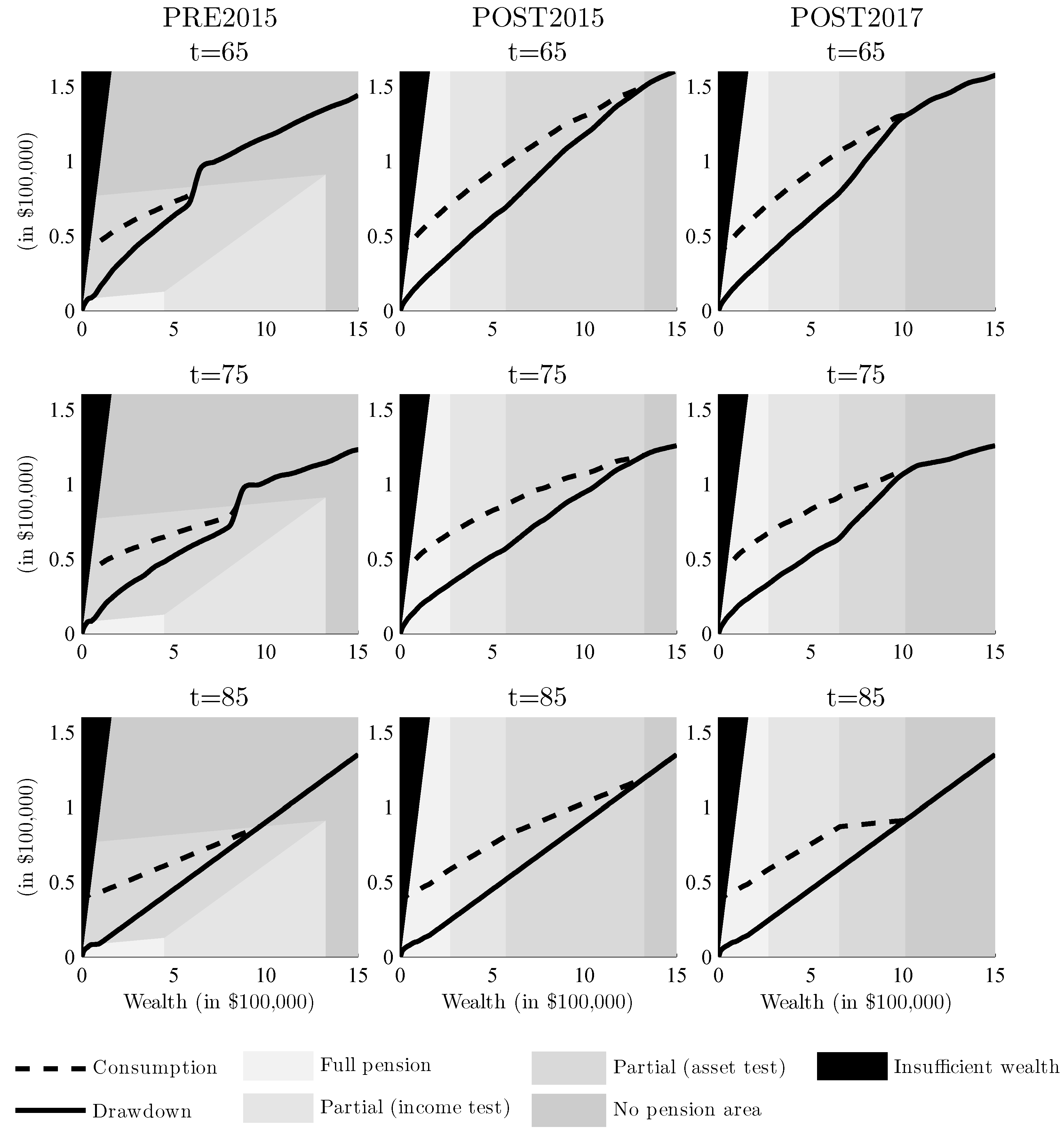
• Policy 1, Pre-January 2015 (PRE2015): The first policy reflects the means-test and policy rules prior to 1 January 2015, which is what the majority of Australian retirees are being tested under. Any drawdown from the Allocated Pension account is counted towards the income-test, where minimum withdrawal rates impose a lower bound on optimal consumption (withdrawals from liquid wealth must be larger or equal to these rates).
• Policy 2, Post-January 2015 (POST2015): This policy focuses on the changes for the income-test of Allocated Pension accounts. The income-test now uses deemed income rather than drawdown; thus, the liquid wealth is used in both the asset and income-test. The retiree can therefore withdraw more liquid wealth without missing out on Age Pension payments.
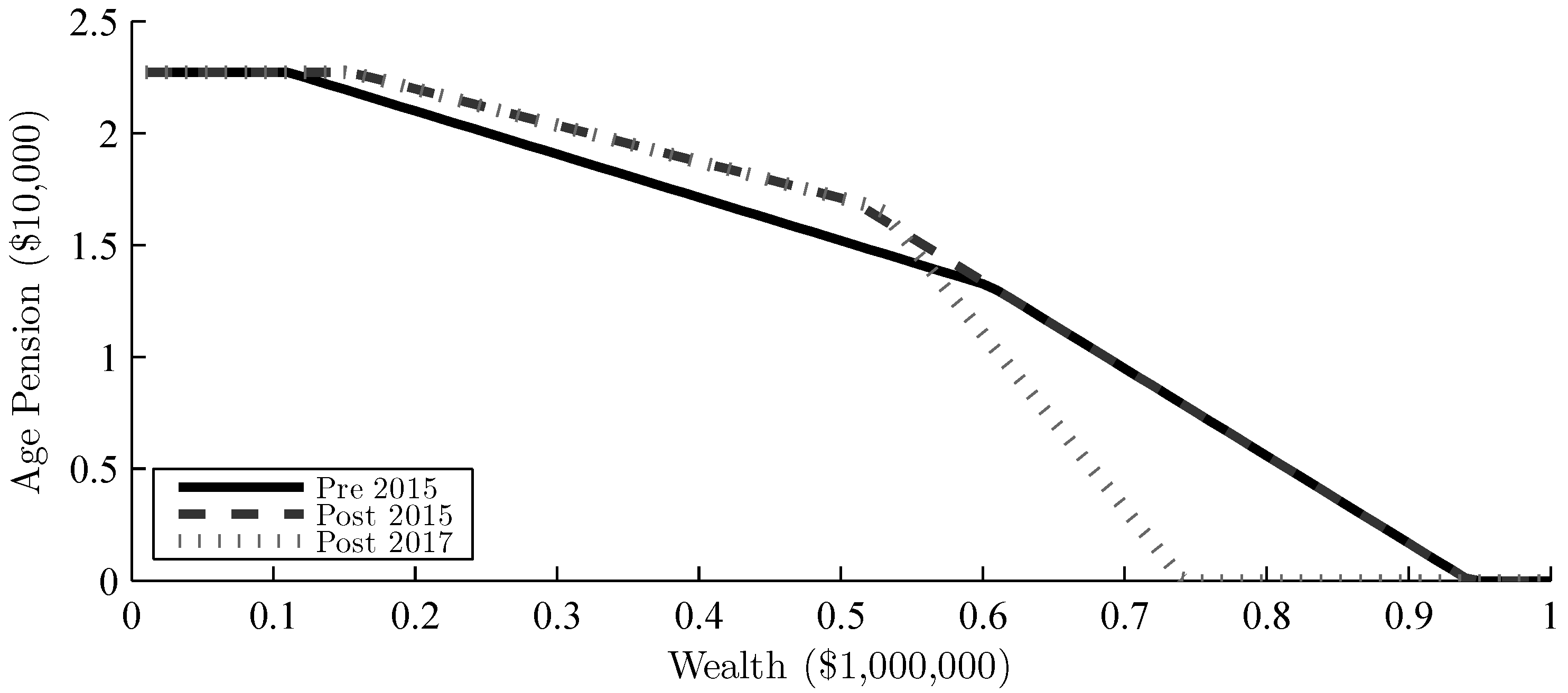
• Policy 3, asset-test changes January 2017 (POST2017): On 1 January 2017, the thresholds of the asset-test were ‘rebalanced’, hence changed significantly. The thresholds for the asset-test increased, and the taper rate doubled. This effectively means that retirees will now receive full Age Pension for a higher level of wealth, but once the asset-test binds, the partial Age Pension will decrease twice as fast, causing them to receive no Age Pension at a lower level of wealth than before. No adjustments were made to the full Age Pension or income-test threshold.

2.3. Age Pension

The Age Pension rules state that the entitlement age is 65 for both males and females9, with the current means-test thresholds and taper rates for January 2017 presented in Table 1 (column ‘POST2017’) and discussed in detail later in this section. All retirees entitled to Age Pension can receive at most the full Age Pension, which decreases as assets or income increases and is determined by the income- and asset-test. All income streams of Allocated Pension accounts opened after 1 January 2015 are now based on deemed income, while accounts opened prior to this are ‘grandfathered’; hence, they will continue to be assessed under the old rules (Department of Social Services 2017). The newer rules have also introduced a ‘work bonus’ deduction for the income-test, but as the model assumes the retiree is no longer in the workforce, this has been left out.

2.3.1. Deemed Income

Deemed income refers to the assumed returns from financial assets, without reference to the actual returns on the assets held. The deemed income only applies to financial assets and account-based income streams and is calculated as a progressive rate of assets. Therefore, the income-test can depend on both labour income (if any), deemed income from financial investments not held in the Allocated Pension account, drawdown from Allocated Pension accounts if opened prior to 2015 or deemed income on such accounts if opened after 1 January 2015.

The deeming rates are subject to change in relation to interest rates and stock market performance10. Two different deeming rates may apply based on the value of the account: a lower rate ${\varsigma }_{-}$ for assets under the deeming threshold ${\kappa }_d$ and a higher rate ${\varsigma }_{+}$ for assets exceeding the threshold, as shown in Table 1.

2.3.2. Age Pension Function

The Age Pension received is modelled with respect to the current liquid assets, where the account value is used for the asset-test. Since the model assumption states that no labour income is possible, all income for the income-test comes from either deemed income (POST2015, POST2017) or generated from withdrawals of liquid assets (PRE2015). The Age Pension function can thus be defined as:

$$P_t:=f\left(W_t\right)=max\left[0,min\left[P_{\max }^d,min\left[P_{\mathrm{A}},P_{\mathrm{I}}\right]\right]\right],$$

(10)

where $P_{\max }^d$ is the full Age Pension, $P_{\mathrm{A}}$ is the asset-test and $P_{\mathrm{I}}$ is the income-test functions. The $P_{\mathrm{A}}$ function is the same for rules prior and post 2015 and is defined as:

$$P_{\mathrm{A}}:=P_{\max }^d-(W_t-L_{\mathrm{A}}^{d,h}){\varpi }_{\mathrm{A}}^d,$$

(11)

where $L_{\mathrm{A}}^{d,h}$ is the threshold for the asset-test and ${\varpi }_{\mathrm{A}}^d$ the taper rate for assets exceeding the thresholds. Superscript d is a categorical index indicating couple or single household status as defined in Equation (7). The variables are subject to whether it is a single or couple household, and the threshold for the asset-test is also subject to whether the household is a homeowner or not ($h=\{0,1\}$). Although the $P_{\mathrm{A}}$ function is the same for both the old and new policies, the $P_{\mathrm{I}}$ function is different. For the deeming rate-based policies, it can be written as:

$$P_{\mathrm{I}}:=P_{\max }^d-(P_{\mathrm{D}}\left(W_t\right)-L_{\mathrm{I}}^d){\varpi }_{\mathrm{I}}^d,$$

(12)

$$P_{\mathrm{D}}\left(W_t\right)={\varsigma }_{-}min\left[W_t,{\kappa }^d\right]+{\varsigma }_{+}max\left[0,W_t-{\kappa }^d\right],$$

(13)

where $L_{\mathrm{i}}^d$ is the threshold for the income-test and ${\varpi }_{\mathrm{I}}^d$ the taper rate for income exceeding the threshold. Function $P_{\mathrm{D}}\left(W_t\right)$ calculates the deemed income, where ${\kappa }_d$ is the deeming threshold, and ${\varsigma }_{-}$ and ${\varsigma }_{+}$ are the deeming rates that apply to assets below and above the deeming threshold, respectively.

To model the Age Pension prior to 2015, when the actual withdrawals from Allocated Pension accounts were used for the income-test instead of deeming rates, the $P_I$ function is defined as:

$$P_{\mathrm{I}}:=P_{\max }^d-({\alpha }_t{W}_t-M\left(t\right)-L_{\mathrm{I}}^d){\varpi }_{\mathrm{I}}^d,$$

(14)

$$M\left(t\right)=\frac{W_{t_0}}{e_{t_0}}{(1+\tilde{r})}^{t_0-t},$$

(15)

where the function $M\left(t\right)$ represents the income-test deduction that was available for accounts opened prior to 2015, $e_{t_0}$ is the lifetime expected at age $t_0$ and $\tilde{r}$ the inflation. As the model is defined in real terms, the future income-test deductions must discount inflation. Function parameters are given in Table 1.

2.4. Parameters

The model parameters are taken from Andreasson et al. (2017), where calibration was performed on empirical data from Australian Bureau of Statistics (2011). However, the consumption floor ${\overline{c}}_d$ and the threshold for luxury bequest a must be adjusted as they represent monetary values. Since the previous model was defined in real terms, we need to set a new base year for the comparison. Therefore, we adjust these parameters based on the Age Pension adjustments from 2010–2016. Currently, the Age Pension payments are adjusted to the higher of the Consumer Price Index (CPI) and Male Average Weekly Total Earnings (MTAWE). The increase in full Age Pension payments from 2010–2016 equals an approximately 4.5% increase per year. We assume that the utility parameters representing monetary values have increased in the same manner. All utility model parameter values are shown in

Table 2. Model parameters where monetary values have been adjusted for 2016.

	${\mathbf{\gamma }}_{\mathit{d}}$	${\mathbf{\gamma }}_{\mathbf{H}}$	$\mathbf{\theta }$	a	${\overline{\mathit{c}}}_{\mathit{d}}$	$\mathbf{\psi }$	$\mathbf{\lambda }$	${\mathbf{\zeta }}_{\mathit{d}}$
Single household	$-1.98$	$-1.87$	0.96	$27,200	$13,284	1.18	0.044	1.0
Couples household	$-1.78$	$-1.87$	0.96	$27,200	$20,607	1.18	0.044	1.3

.

On 1 January 2017, the thresholds of the asset-test were ‘rebalanced’, hence changed significantly (Australian Government Department of Veterans’ Affairs 2017). The thresholds for the asset-test were increased, and the taper rate ${\varpi }_{\mathrm{A}}^d$ doubled. Age Pension parameters do not have to be adjusted other than updating the asset-test thresholds and taper rate according to the changes, as Age Pension payments remained the same. The parameters for the Age Pension for all policies are shown in Table 1. The model will be solved for two different cases of expected returns: a lower real risky return that follows $Z_t\sim \mathcal{N}(0.0325,0.133)$, which corresponds to an overall portfolio return less than the deeming rate, and a higher real risky return that follows $Z_t\sim \mathcal{N}(0.06,0.133)$ to generate a portfolio return equal to or above the deeming rate. We are using the standard deviation from yearly returns in S&P/ASX200 Total Return and the deposit rate, both estimated in Andreasson et al. (2017). The real risk-free rate is set to $r_t=0.005$. While a lower mean return often has lower variance, we are using one variance for both return cases as the comparative results between the policies remains the same. In addition to this, we set the following.

-

A retiree is eligible for Age Pension at age $t=65$ and lives no longer than $T=100$.

-

The lower threshold for housing is set to $30,000. That is, a retiree with wealth below this level cannot be a homeowner, hence $H\in \{0,[$30,000$,\mathrm{W}\left]\right\}$.

-

A unisex survival probability is used to avoid separating the sexes, as it would add an extra state variable. The survival probabilities for a couple are assumed to be mutually exclusive, based on the oldest partner in the couple. The actual mortality probabilities are taken from Life Tables published by Australian Bureau of Statistics (2014).

-

The subjective discount rate $\beta$ is set in relation to the real interest rate so that $\beta =e^{-{\sum }_{i=t}^{t^{\prime }}{r}_i}$.

Minimum withdrawal rates for Allocated Pension accounts are shown in

Table 3. Minimum regulatory withdrawal rates for Allocated Pension accounts for the year 2017 and onwards (https://www.ato.gov.au/rates/key-superannuation-rates-and-thresholds/?page=10, accessed June 5, 2017).

Age	≤64	65–74	75–79	80–84	85–89	90–94	≤95
Min. drawdown	4%	5%	6%	7%	9%	11%	14%

(Australian Taxation Office 2016). The rates impose a lower bound on optimal consumption; therefore, withdrawals from liquid wealth must be larger or equal to these rates.

2.5. Numerical Implementation

The model is solved numerically. By discretising the wealth and house state on a grid of k log-equidistant grid points $W_0,\dots ,W_k$ and $H_0,\dots ,H_k$ for each year $t=t_0,\dots ,T$ and by writing Equation (6) as a Bellman equation, the problem is solved recursively with backward induction. The lower bound of the grid is set to $1; the upper bound $H_k$ is chosen to equal total wealth $\mathsf{W}$; and the upper bound $W_k$ is chosen large enough so that values close to the upper bound have no material effect on the range of wealth in the analysis. Extrapolation is therefore less important when integrating risky returns, and the interpolation between grid points is done with the shape-preserving Piecewise Cubic Hermite Interpolation Polynomial (PCHIP) method, which preserves the monotonicity and concavity of the value function (Kahaner et al. 1988). The expectation with respect to the stochastic return is calculated with the Gauss–Hermite quadrature using five nodes. For each grid point in the wealth and house state, optimal drawdown proportions ${\alpha }_t$ and risky asset allocation ${\delta }_t$ are found using a two-dimensional optimisation. For a more detailed description of the numerical solution, see Andreasson et al. (2017).

3. Results

The model is solved each year, with respect to optimal decisions for each policy and expected return and for each combination of single/couple and homeowners/non-homeowner households. The income-test changes in POST2015 lead to some interesting implications for the retirees in all three decision variables (housing, consumption and risky asset allocation), due to the assets now being included twice in the means-test.

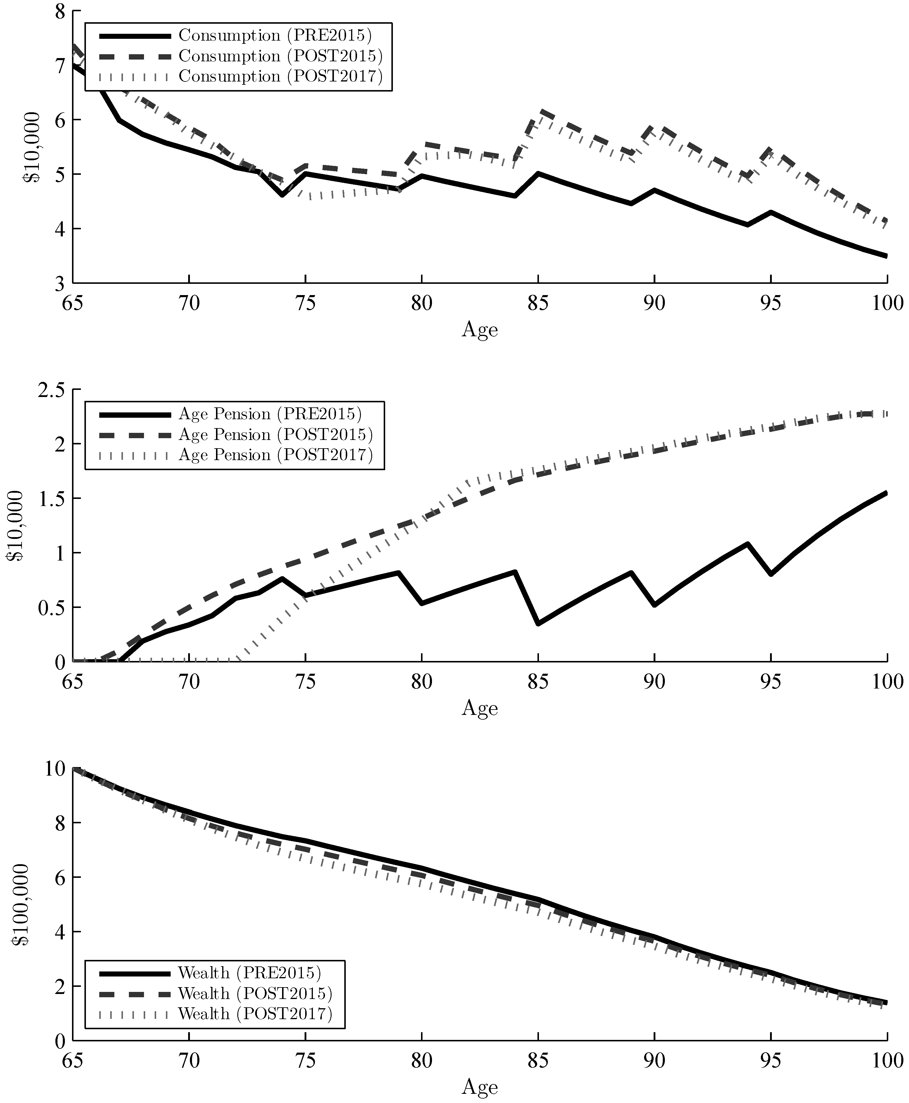
3.1. Optimal Consumption

The optimal consumption consists of the drawdown from liquid wealth and the Age Pension received and exemplifies a behaviour consistent with traditional utility models. Figure 1 shows the optimal consumption and drawdown for a given liquid wealth under each of the three policies. The grey areas in the background indicate whether any means-test is binding. As can be seen, only PRE2015 is subject to the size of the drawdown in the income test, while the other policies depend on liquid wealth only. The curve is generally a smooth, concave and monotone function of wealth. The curve becomes flatter as the retiree ages, which is the desired effect from the model’s “health” proxy as to reflect the lower consumption resulting from decreasing health. However, this general behaviour starts to deviate as the retiree ages due to the minimum withdrawal rates. For a retiree aged 65 with an account of $500,000, the optimal consumption for a non-homeowner couple under the current (POST2017) policy is roughly 13%, which is more than the minimum withdrawal rate of 5% (Table 3). As the retiree ages, his/her consumption tends to decrease, but around age 85, the minimum withdrawal rates cross over the optimal consumption; hence, the drawdown curve becomes proportional to wealth. This is in line with Bateman et al. (2007), which finds that welfare decreases slightly when minimum withdrawal rules are enforced over unconstrained optimal withdrawals, especially for higher levels of risk aversion. This deviation occurs at an even earlier age for singles and wealthier retirees.

There are a couple of distinct differences in drawdown behaviour between the policies; however, no apparent differences were identified between homeowner or non-owners or between low and high expected return. Single and couple households had the same behaviour with respect to the means-test thresholds, although at different dollar values. For an illustration of the differences, we therefore only use the case of a couple non-homeowner household. First, consumption is higher for the policies that base the income-test on deeming rates. For a given level of drawdown, deeming rates tend to pay more Age Pension, even for the harsher POST2017 rules. This is because a certain wealth would attract higher penalties in the means-test when drawdown is used, compared to deemed income for the same wealth. Second, the deeming rate-based policies show low-to-no sensitivity to the means-test thresholds, indicating that the retiree can no longer plan their consumption behaviour to optimise Age Pension payments. This is in contrast to PRE2015, which shows that drawdown was highly sensitive to the means-test and could be utilised in financial planning (Andreasson et al. 2017). There is a marginal effect when the retiree goes from no Age Pension to receiving partial Age Pension, especially for the 2017 asset-test adjustment, shown as a tiny dent where the consumption and drawdown curve intersect (the threshold between no pension and partial pension due to asset-test). This implies that a retiree should consume slightly more when his/her wealth is close to this threshold in order to receive partial Age Pension, but the additional utility would be so small that it is negligible in planning. The same behaviour can be expected to occur when the income-test binds over the asset-test (the threshold between partial pension due to income-test and asset-test), which can be seen as a slight change in the drawdown curve due to different taper rates for the partial Age Pension, but no apparent effect is identified in the consumption.

Although the low and high expected return had no effect on optimal drawdown, it does have a significant effect over the lifespan of a retiree. Figure 2 and Figure 3 show the consumption and wealth paths over time for the low and high expected return respectively, as well as the Age Pension payments. The zigzag pattern in the consumption is due to the minimum withdrawal rates, which increase every five years and start to bind around age 75. The higher return leads to a flatter wealth path initially, irrespective of policy, while it is declining steadily for the lower return. The level of consumption shows a similar shape in both graphs, declining early in retirement, but increasing later on due to minimum withdrawals. The consumption is significantly higher with the higher expected return (due to a higher level of wealth) and even exceeds the initial consumption. As indicated in Figure 1, consumption also tends to be higher for the deeming rate policies, even if the wealth decumulation is in line with PRE2015. These characteristics are all expected in the model, but the interesting part is the effect that the policies and expected return have on Age Pension payments. As wealth paths throughout retirement are almost identical, the difference in consumption is mainly due to additional Age Pension under the newer policies. Even if the pension function for POST2017 seems to results in less Age Pension for higher levels of wealth (see Figure 4), in practice, this is not the case. The PRE2015 policy penalizes drawdown very hard and leads to significantly less Age Pension over all. As the minimum withdrawal rate increases with age, the difference in partial Age Pension increases, as well. The POST2015 policy leads to a larger amount of Age Pension at (almost) all times, and the retiree is still better off with PRE2017 despite having a more aggressive taper rate. If the deeming rates are lower than the return on assets, the retiree will receive more Age Pension towards the end of his.her retirement. Even so, the minimum withdrawal at this point would be high enough that any additional Age Pension received would still not increase the consumption. It is only for less wealthy households that deeming rates have an effect on the Age Pension payments throughout retirement, but even for these households, the minimum withdrawal rates bind around age 75; hence, they will have less additional utility in terms of consumption.

One of the reasons for changing the policy was for the government to generate savings, but the deeming rules will not have the desired outcome on Allocated Pension accounts unless the deeming rates increase. Even in the case where returns are less than the deeming rates, the retiree is better off than before as deemed income in the means-test will be less than actual drawdown early in retirement. As a result, the retiree will receive more Age Pension for a given level of wealth than before. Only when the minimum withdrawals are removed (or at least decreased), which in turn could lead to lower withdrawals for given wealth levels, could current rates lead to Age Pension payments being less under the new policy11. Under the PRE2015 policy, the relatively high drawdown for the retiree would most often lead to no Age Pension due to the income-test, while under the deeming rate-based policies, the retiree would receive a significant amount of Age Pension throughout retirement.

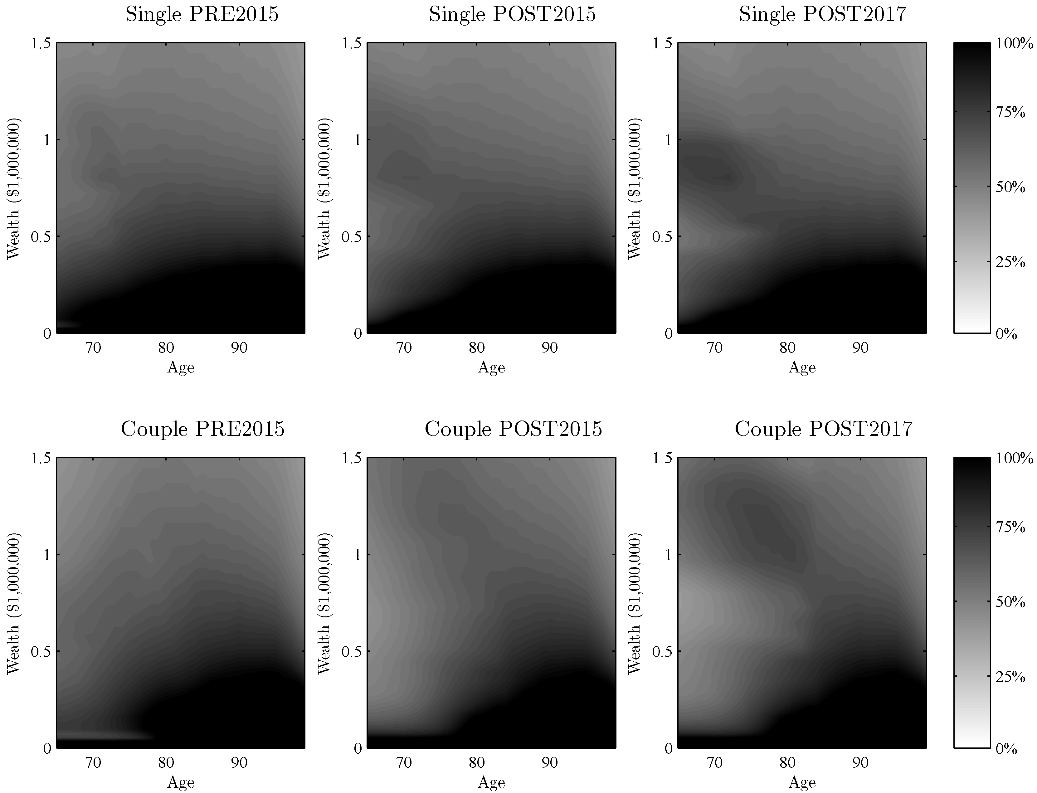
3.2. Optimal Risky Asset Allocation

The risky allocation displays similar characteristics in all policies and is essentially the same for homeowners and non-homeowners, but differs between singles and couples. The level of expected returns does not result in any difference in the shape of the risky asset allocation surface, but it does affect the average allocation. Figure 5 shows the optimal risky allocation given age and liquid wealth. A higher expected return leads to a higher overall allocation to risky assets, but the comparatively darker and lighter areas remain the same. High or low deeming rates have no observable effect on risky asset allocation. The exposure to risky assets in the portfolio is however highly dependent on wealth and age, and even more so compared to PRE2015. This is expected since the means-test is now based on wealth in both the asset and the income-test, which means investment returns will have a larger impact on expected utility.

The optimal allocation surface is characterised by the expected marginal utility from the consumption and bequest utility. The black bottom area to the left (Figure 5) suggests 100% allocation to risky assets for low levels of wealth, where the upper bound of the area corresponds to maximum margin utility from the consumption function . The upper bound to the right is the maximum marginal utility from bequest, which occurs at a higher level than for consumption ($\sim$ $450,000). Up to these levels, it is therefore optimal to allocate 100% to risky assets, as the reward is larger than the risk as a result of the ‘buffer’ effect. This buffer occurs when the decreasing wealth that stems from an investment loss is partially offset via increased Age Pension and can be seen as the comparatively darker area towards the top left (indicating where partial pension becomes no pension) in Figure 5. The buffer effect is, therefore, strongest for a retiree who has no Age Pension, but is close to receiving partial Age Pension. An investment loss, in this instance, would be offset by partial Age Pension, whereas an investment profit would not cause the retiree to miss out on Age Pension that he/she would otherwise receive. The taper rate is steeper for the asset-test than the income-test (especially for POST2017); hence, marginal utility is lower when the asset-test is binding and results in a higher contrast surface. For very low levels of wealth, the buffer effect is the opposite; investment losses can never lead to more than full Age Pension, and investment profits will decrease the amount of partial Age Pension received. Again, this is especially present in POST2017 and can be seen as the comparatively whiter area towards the bottom left.

Another interesting effect occurs as the minimum withdrawal rates cross above unconstrained optimal drawdown. When the retiree is forced to withdraw more from his/her account than is optimal to consume, the marginal utility drops significantly. This occurs approximately at age 75 for both single and couple households, although slightly later for less wealthy households. The marginal utility received from consumption is essentially zero after this age. Thus, the utility consists of an increasingly larger proportion of bequest as the retiree ages (and mortality risk increases). This switch occurs where the bottom black area starts to increase towards the right, as it moves from utility from consumption to utility from bequest. Once the minimum withdrawal rates exceed the non-constrained optimal drawdown, the different policies become nearly identical as minimum withdrawal rates bind. The difference is therefore only for the initial years of retirement, ages 65–80, due to the way the income-test is constructed. In regard to POST2017, the buffer feature is slightly stronger owing to the steeper taper rate, but the characteristics are similar to the other policies.

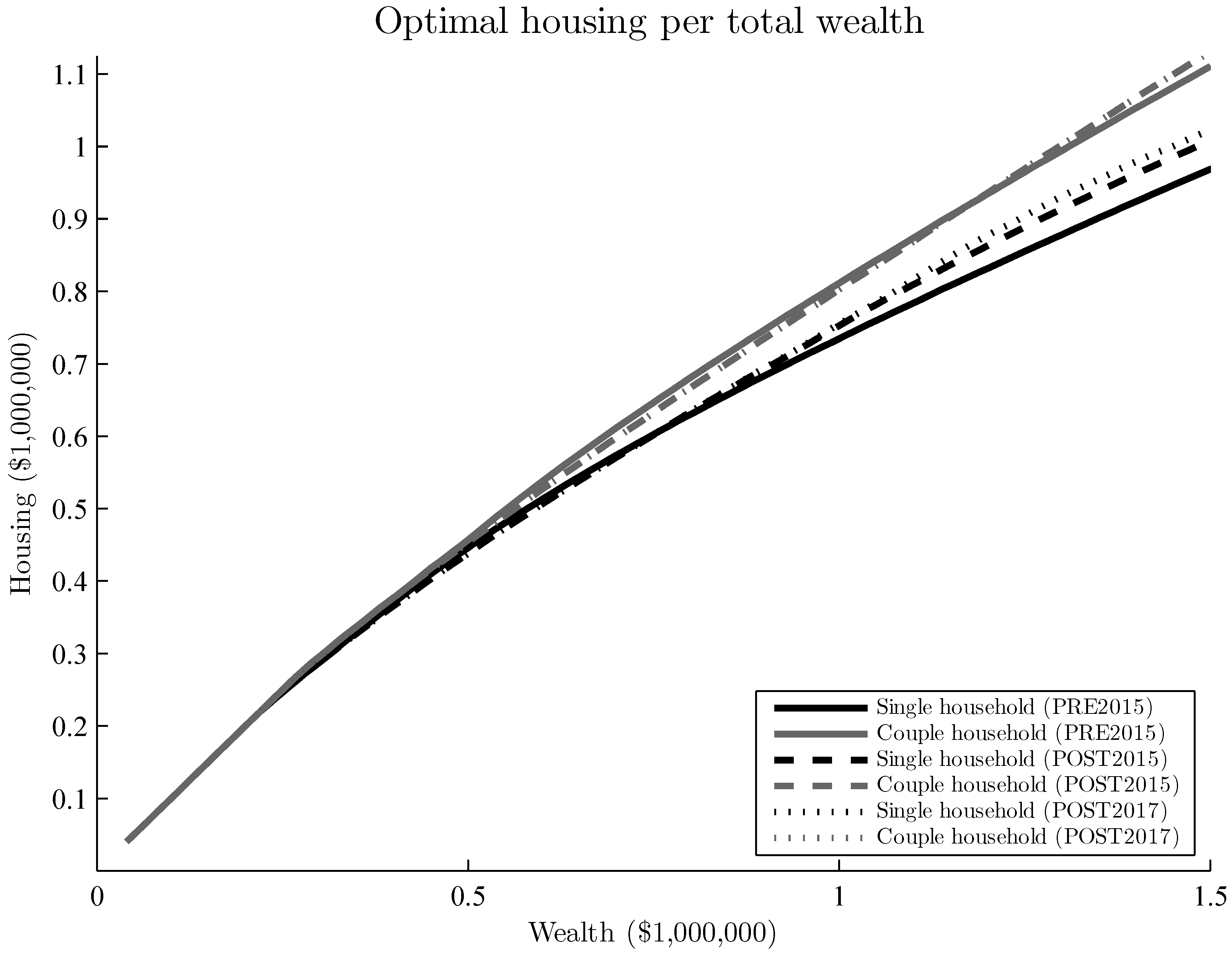
3.3. Optimal Housing Allocation

The decision variable for the allocation of assets into a family home is expected to change slightly due to the increased focus on assets in the means-test. With respect to expected returns and deeming rate levels, however, the optimal allocation is unchanged. The decision made at the time of retirement shows that under the newer policy rules (POST2015, POST2017), it is optimal to invest marginally less than under PRE2015, up to a total wealth level of approximately $735,000 for single households and $1,155,000 for couple households (see Figure 6). This would leave approximately $144,000 and $247,000 respectively as liquid wealth. Households with total wealth above this level, meanwhile, are recommended to invest slightly more. These allocation decisions leave liquid wealth just below the thresholds for receiving full Age Pension, and the difference in the housing curves can be explained by the income-test changes. For a given wealth, the deeming rate-based policies provide the retiree with more partial pension than with PRE2015. Early in retirement, the optimal consumption is high, which causes the income-test to bind under the PRE2015 policy. The deemed income is much lower than drawdowns, which ultimately results in more partial Age Pension. Since a certain level of liquid wealth under the POST2015 and POST2017 policies will lead to higher expected utility, it is optimal to allocate slightly more to housing (as long as the liquid wealth is not very low) to benefit from receiving additional partial Age Pension. The effects of POST2017 are only marginally larger than POST2015; thus, the steeper taper rates do not impact the housing allocation decision materially.

3.4. Limitations

The analysis is dependent on the assumptions made in the model. The optimal controls show very low sensitivity to many of the assumptions, such as the choice of process for risky returns and constant house value in real terms. While the overall shape of the risky asset allocation surface (see Figure 5) remains the same given alternative return distributions and volatility, the average level of risky asset allocation increases with risky return and decreases with volatility. The model is more sensitive to the relation between risk aversion parameters than to the absolute vale of any parameter. Most of the main characteristics in the results, such as decreasing sensitivity to the means-test with age and binding minimum withdrawal rates, do not change given slightly different utility parameters or levels of return. The absolute levels are, however, subject to parametrisation and will differ for each individual. Since the calibration of the model in Andreasson et al. (2017) was shown to fit the empirical data for Australian retirees well, we believe that this analysis can reflect the general behaviour of Australian retirees and at least provide important insights into the effects from different Age Pension policies.

We acknowledge that there might be models more suitable to explain the individual behaviour in retirement. By basing the model on the standard utility theory, it is possible that the preferences of the retirees are not properly captured even if the model is well calibrated to data. Risk averse utility functions tend to be concave, but micro economics suggests that the true utility curve is S-shaped. We use the standard utility theory as we can calibrate this model using the available empirical data. However, the model can benefit from being extended with stochastic dominance theory (Kopa et al. 2016; Levy 2006) or prospect theory (Kahneman and Tversky 1979), in order to avoid the inherent limitations of the standard utility theory. This is the subject of future research.

4. Conclusions

In this paper, we adapt the expected utility life cycle model from Andreasson et al. (2017) to account for the Age Pension policy changes in Australia since 2015, including the new steeper taper rates for the asset-test in force since 2017. These changes apply to all Allocated Pension accounts opened after 1^st of January 2015 and affect the treatment of income for the Age Pension income-test, which leads to different optimal decisions for consumption, investments and housing. In addition, we also evaluate the effect of the deeming rate levels in relation to portfolio returns.

We find that optimal consumption only applies early in retirement, as minimum withdrawal rates exceed unconstrained optimal drawdown rates for ages 75–85, depending on wealth level. While it is possible to plan withdrawals for maximum utility prior to this point, these possibilities are almost non-existent under the deeming rate-based policies compared with the previous drawdown-based policy. Optimal drawdown equals minimum withdrawal after age 85 (as it becomes a binding lower constraint for withdrawal); thus, the policies are identical after this age. That said, since the income-test tends to bind for the old rules while the asset-test dominates for the new rules, the retiree will now receive more partial pension throughout retirement. Even with the steeper taper rate introduced January 2017, the retiree can consume more while drawing down less assets, thanks to a more generous Age Pension compared.

Since income (which was considered as drawdown from the Allocated Pension account before 2015) is now replaced by deemed income, the assets are means-tested twice, resulting in the risky asset allocation becoming more sensitive. The changes in optimal risky asset allocation over time and wealth are similar under all policies, but the changes are more aggressive with the steeper 2017 taper rates. This is due to the marginal utility from consumption and bequest, which has increased due to the taper rate, as well as the level of buffering against investment losses the Age Pension provides. This effect is only present in the first part of retirement and dies off as the minimum withdrawal rates bind where the bequest motive becomes more important.

It is optimal to invest slightly more in housing under the deeming rate-based policies, provided that the retiree’s remaining liquid wealth is close to (or higher) than the threshold between full and partial Age Pension at the time of retirement. This will allow the retiree to receive more partial Age Pension and to increase his/her expected utility in the long term. If the retiree instead has lower total wealth than the threshold, he/she is alternatively recommended to invest marginally less than before.

With respect to higher and lower expected risky asset returns and high and low deeming rates in relation to the expected returns, optimal decisions tend to be very robust. Neither optimal drawdown, deeming rates nor housing allocating showed sensitivity to the expected return. Risky asset allocation, on the other hand, adjusts the average allocation based on expected return, but does not change in relation to the deeming rates. It is important to put all decisions in context, however, in order to understand how high and low returns and deeming rates affect the retiree. Even if optimal drawdown for a given wealth remains constant, the additional Age Pension received from lower deeming rates can increase the overall consumption. However, this tends to occur later in retirement where higher consumption is not as common; hence, the retiree is only marginally better off.

One surprising finding is that a retiree with an income stream where minimum withdrawal rules are enforced will receive more Age Pension over the course of his/her lifetime with the deeming rate-based policies. Due to the minimum withdrawal requirement, the drawdown tends to be higher than what is optimal for most ages, which under the drawdown-based rules would result in no or low partial Age Pension. The deeming rate-based policies will generate significant Age Pension payments from the same drawdown and wealth levels, irrespective of whether the deeming rates are high or low in relation to returns. This makes the government’s goal to reduce the budget difficult to reach. As the retiree is less sensitive to deeming rates than minimum withdrawal rates, our simulations suggest that both the retiree and the government would be better off by lowering the minimum withdrawal rates rather than the deeming rates. However, the goal of reducing incentives for maximising Age Pension payments and focusing on maximising total disposable income is met: the deeming rate based policies are not as sensitive to optimal withdrawal decisions in order to maximise Age Pension payments as the old policy was. The possibility of planning decisions around the means-test has therefore moved from optimal consumption to optimal risky asset allocation, owing to the steeper taper rates.

The analysis can easily be extended to suit the defined-contribution pension system in other countries by adjusting the Age Pension function and necessary constraints and assumptions. This would allow for a comparative analysis between Australia’s Age Pension and similar countries or evaluating a specific means-tested pension policy individually. A particularly interesting case would be the comparison with the U.S. pension systems. The assumptions for the Allocated Pension account need to be adjusted to match those of an ‘Individual Retirement Account’ or 401(k)12, and the Age Pension needs to be replaced with the Supplemental Security Income and its associated means-test function. Thus, investigating other policies globally will be a subject for future research.

All authors contributed equally to this research work by providing new ideas, writing the paper, discussing existing results and sharing their knowledge in this field. Numerical calculations were performed by Johan Andreasson.

References

1. Andreasson, Johan G., Pavel V. Shevchenko, and Alex Novikov. 2017. Optimal Consumption, Investment and Housing with Means-tested Public Pension in Retirement. Insurance Mathematics and Economics 75: 32–47. [Google Scholar] [CrossRef]
2. Australian Bureau of Statistics. 2011. Household Expenditure Survey and Survey of Income and Housing Curf Data. Available online: http://www.abs.gov.au/ausstats/[email protected]/mf/6503.0 (accessed on 6 June 2014).
3. Australian Bureau of Statistics. 2014. 3302.0.55.001 - Life Tables, States, Territories and Australia, 2012–2014. Available online: http://www.abs.gov.au/ausstats/[email protected]/mf/3302.0.55.001 (accessed on 4 November 2014).
4. Australian Government Department of Veterans’ Affairs. 2017. Rebalanced Assets Test to Apply from 2017. Available online: http://www.dva.gov.au/rebalanced-assets-test-apply-2017/ (accessed on 19 January 2017).
5. Australian Taxation Office. 2016. Minimum Annual Payments for Super Income Streams. Available online: https://www.ato.gov.au/rates/key-superannuation-rates-and-thresholds/ (accessed on 27 October 2016).
6. Bateman, Hazel, Susan Thorp, and Geoffrey Kingston. 2007. Financial engineering for Australian annuitants. In Retirement Provision in Scary Markets, 1st ed. Edited by Hazel Bateman. Northampton: Edward Elgar Publishing, pp. 123–44. [Google Scholar]
7. Blake, David, Douglas Wright, and Yumeng Zhang. 2014. Age-dependent investing: Optimal funding and investment strategies in defined contribution pension plans when members are rational life cycle financial planners. Journal of Economic Dynamics and Control 38: 105–24. [Google Scholar] [CrossRef]
8. Boender, G. C., P. C. van Aalst, and F. Heemskerk. 1997. Modelling & Management of Assets & Liabilities of Pension Plans in the Netherlands. Rotterdam: Erasmus University Rotterdam. [Google Scholar]
9. Cocco, João, and Francisco Gomes. 2012. Longevity risk, retirement savings, and financial innovation. Journal of Financial Economics 103: 507–29. [Google Scholar] [CrossRef]
10. Cocco, João, Francisco Gomes, and Pascal Maenhout. 2005. Consumption and portfolio choice over the life cycle. Review of Financial Studies 18: 491–533. [Google Scholar] [CrossRef]
11. Department of Social Services. 2017. Guides to Social Policy Law. Available online: http://guides.dss.gov.au/guide-social-security-law (accessed on 4 January 2017).
12. Ding, Jie. 2014. Essays on Post-Retirement Financial Planning and Pension Policy Modelling in Australia. Ph.D. Dissertation, Macquarie University, Sydney, Australia. [Google Scholar]
13. Ding, Jie, Geoffrey Kingston, and Sachi Purcal. 2014. Dynamic asset allocation when bequests are luxury goods. Journal of Economic Dynamics and Control 38: 65–71. [Google Scholar] [CrossRef]
14. Dupačová, Jitka, and Jan Polívka. 2009. Asset-liability management for Czech pension funds using stochastic programming. Annals of Operations Research 165: 5–28. [Google Scholar] [CrossRef]
15. Fisher, Lance. 1930. The Theory of Interest: As Determined by Impatience to Spend Income and Opportunity to Invest it, (1 ed.). New York: The Macmillan Company. [Google Scholar]
16. Henry, Ken. 2009. Australia’s Future Tax System—Report to the Treasurer (Overview). Technical Report December, Commonwealth of Australia. Available online: http://taxreview.treasury.gov.au/content/downloads/ (accessed on 20 April 2017).
17. Hilli, Petri, Matti Koivu, Teemu Pennanen, and Antero Ranne. 2007. A stochastic programming model for asset liability management of a Finnish pension company. Annals of Operations Research 152: 115–39. [Google Scholar] [CrossRef]
18. Hulley, Hardy, Rebecca Mckibbin, Andreas Pedersen, and Susan Thorp. 2013. Means-Tested Public Pensions, Portfolio Choice and Decumulation in Retirement. Economic Record 89: 31–51. [Google Scholar] [CrossRef]
19. Iskhakov, Fedor, Susan Thorp, and Hazel Bateman. 2015. Optimal Annuity Purchases for Australian Retirees. Economic Record 91: 139–54. [Google Scholar] [CrossRef]
20. Kahaner, David, Cleve Moler, Stephen Nash, and George Forsythe. 1988. Numerical Methods and Software. Upper Saddle River: Prentice Hall. [Google Scholar]
21. Kahneman, Daniel, and Amos Tversky. 1979. Prospect Theory: An Analysis of Decision under Risk. Econometrica 47: 263–92. [Google Scholar] [CrossRef]
22. Kopa, Miloš, Vittorio Moriggia, and Sebastino Vitali. 2016. Individual optimal pension allocation under stochastic dominance constraints. Annals of Operations Research 14: 1–37. [Google Scholar] [CrossRef]
23. KPMG. 2010. KPMG Econtech CGE Analysis of the Current Australian Tax System. Technical Report March. Available online: https://www.cpaaustralia.com.au (accessed on 17 September 2016).
24. Levy, Haim. 2006. Investment Decision Making under Uncertainty, 2nd ed. Dordrecht: Springer. [Google Scholar]
25. Lockwood, Lee. 2014. Incidental Bequests: Bequest Motives and the Choice to Self-Insure Late-Life Risks. NBER Working Paper No. 20745. [Google Scholar] [CrossRef]
26. Merton, Robert. 1969. Lifetime Portfolio Selection Under Uncertainty: The Continuous Time Case. Review of Economics and Statistics 51: 247–57. [Google Scholar] [CrossRef]
27. Merton, Robert. 1971. Optimum consumption and portfolio rules in a continuous-time model. Journal of Economic Theory 3: 373–413. [Google Scholar] [CrossRef]
28. Modigliani, Franco, and Richard Brumberg. 1954. Utility Analysis and the Consumption Function: An Interpretation of Cross-Section Data. In Post Keynesian Economics. Edited by Kenneth K. Kurihara. London: George Allen & Unwin, pp. 388–436. [Google Scholar]
29. Plan For Life. 2016. Report on the Australian Reitrement Income Market. Technical Report, Plan For Life. Available online: http://www.pflresearch.com.au (accessed on 3 April 2016).
30. Rice Warner. 2015. Quo Vadis? Superannuation needs effective policy...not politics. Submission to Tax White Paper Task Force. Available online: http://ricewarner.com/wp-content/uploads/2015/07/Tax-White-Paper.pdf (accessed on 20 April 2017).
31. Samuelson, Paul. 1969. Lifetime portfolio selection by dynamic stochastic programming. The Review of Economics and Statistics 51: 239–46. [Google Scholar] [CrossRef]
32. Shevchenko, Pavel V. 2016. Analysis of Withdrawals From Self-Managed Super Funds Using Australian Taxation Office Data; CSIRO Technical Report EP164438; Canberra: CSIRO Australia.
33. Spicer, Alexandra, Olena Stavrunova, and Susan Thorp. 2016. How Portfolios Evolve after Retirement: Evidence from Australia. Economic Record 92: 241–67. [Google Scholar] [CrossRef]
34. The Commonwealth of Australia. 2015. Budget 2015 Overview. Technical Report. Available online: http://www.budget.gov.au (accessed on 1 October 2014).
35. Vitali, Sebastino, Vittorio Moriggia, and Miloš Kopa. 2017. Optimal pension fund composition for an Italian private pension plan sponsor. Computational Management Science 14: 135–60. [Google Scholar] [CrossRef]
36. Yaari, Menahem. 1964. On the consumer’s lifetime allocation process. International Economic Review 5: 304–17. [Google Scholar] [CrossRef]
37. Yaari, Menahem. 1965. Uncertain Lifetime, Life Insurance, and the Theory of the Consumer. The Review of Economic Studies 32: 1–137. [Google Scholar] [CrossRef]
1
Certain account types for retirement savings have a minimum withdrawal rate once the owner is retired.
2
The pension system in Australia is called ‘superannuation’.
3
The recommendations to introduce deeming was made in Henry (2009), where the fiscal sustainability is evaluated with the general equilibrium model ‘KPMG Econtech MM900’ (KPMG 2010). The model shows the estimation over a 10-year window; hence, we do not know the short-term or year-to-year estimates. In addition to this, the model includes additional suggested tax- and budget-related changes; hence, the effect of introducing deeming rates cannot be isolated.
4
As of 4 May 2017, the current three-month rate offered by Commonwealth Bank is 2.05% (https://www.commbank.com.au/personal/accounts/term-deposits/rates-fees.html, accessed on June 8, 2017).
5
By defining the model in real terms (adjusted for inflation), time-dependent variables do not have to include inflation, which otherwise would be an additional stochastic variable.
6
Note that the purpose is not to model health among the retirees, but rather to explain decreasing consumption with age.
7
The risk aversion is considered to be the same as consumption risk aversion for singles since a couple is expected to become a single household before bequeathing assets.
8
Because the marginal utility is constant for the bequest utility with zero wealth, in a model with perfect certainty and CRRA utility, the optimal solution will suggest consumption up to level a before it is optimal to save wealth for bequest (Lockwood 2014).
9
As of 1 July 2017, this increased to 65.5 years for people born after 1 July 1952, but for our dataset, the entitlement age was 65. Already retired Australians might have had earlier entitlement ages.
10
The current rates are at a historical low. In 2008, the deeming rates ς / ς + were as high as 4%/6%, but in March 2013, they were set to 2.5%/4% due to decreasing interest rates, then in November 2013 to 2%/3.5% and to the current levels of 1.75%/3.25% in March 2015. Note that despite the model being defined in real terms, it can be shown with simple algebra that the deeming rates shall not be adjusted to ‘real’ deeming rates.
11
It should be noted that the findings are for the account-based pension only, as other products that do not enforce the minimum withdrawal rates could incur additional savings for the government under the new rules.
12
A 401(k) is a defined-contribution retirement savings plan sponsored by the employer.
Figure 1. Optimal drawdown and consumption for non-homeowner couple households for a given liquid wealth at the age t, under the three different policy scenarios in the case of low returns ( μ = 0.0325).
Risks 05 00047 g001
Figure 2. Comparison of consumption, Age Pension and wealth over a retiree’s lifetime with the three different policy scenarios. The retiree starts with $1m liquid wealth, which grows with the low expected return each year ( μ = 0.0325), and drawdown follows the optimal drawdown paths under each policy.
Risks 05 00047 g002
Figure 3. Comparison of consumption, Age Pension and wealth over a retiree’s lifetime with the three different policy scenarios. The retiree starts with $1m liquid wealth, which grows with the high expected return each year ( μ = 0.06), and drawdown follows the optimal drawdown paths under each policy.
Risks 05 00047 g003
Figure 4. Comparison of the Age Pension function with the three policy scenarios, based on a single household aged 65–74 and where consumption is assumed to be the minimum withdrawal rate of 5%.
Risks 05 00047 g004
Figure 5. Optimal risky allocation for non-homeowner single and couple household, under each policy, given the low expected return ( μ = 0.0325).
Risks 05 00047 g005
Figure 6. Optimal housing allocation given by total wealth W for single and couple households, under the three policy scenarios with the low return ( μ = 0.0325).
Risks 05 00047 g006