Analyzing the Gaver—Lewis Pareto Process under an Extremal Perspective

Abstract

Pareto processes are suitable to model stationary heavy-tailed data. Here, we consider the auto-regressive Gaver–Lewis Pareto Process and address a study of the tail behavior. We characterize its local and long-range dependence. We will see that consecutive observations are asymptotically tail independent, a feature that is often misevaluated by the most common extremal models and with strong relevance to the tail inference. This also reveals clustering at “penultimate” levels. Linear correlation may not exist in a heavy-tailed context and an alternative diagnostic tool will be presented. The derived properties relate to the auto-regressive parameter of the process and will provide estimators. A comparison of the proposals is conducted through simulation and an application to a real dataset illustrates the procedure.

1. Introduction

Increased exposure to catastrophic losses and the complexity of financial instruments require sophisticated risk assessment tools in areas such as (re) insurance, banking, finance, among others. Extreme value theory plays an important methodological role in risk management by providing appropriate instruments to deal with values as large as or even higher than those ever observed. These techniques include heavy-tailed models and measures to evaluate tail dependence, namely to infer to what extent the occurrence of a risk value in some variable influences an analogous occurrence in another variable.

Linear ARMA (autoregressive moving average) with heavy-tailed noise may be suitable to model time series presenting peaks of observations. However, in place of a summation, a maximum operator is more propitious to derive extremal properties. Max-autoregressive and moving maximum models were developed within this spirit, such as MARMA (max-autoregressive moving average) introduced in Davis and Resnick (1989) and M4 (multivariate maxima of moving maxima) processes presented in Smith and Weissman (1996). The Pareto model, which is closed under geometric multiplication and minimization, also motivated the first-order Pareto processes presented in Arnold (2001). Further analysis may be found in Ferreira (2016) and references therein.

A random variable (rv) is modeled by Pareto($\mathsf{\sigma },\mathsf{\alpha }$) if it has distribution function (df)

$$\begin{array}{c}\hfill F_X\left(x\right)=1-{(x/\mathsf{\sigma })}^{-\mathsf{\alpha }},x>\mathsf{\sigma },\mathsf{\sigma }>0,\mathsf{\alpha }>0.\end{array}$$

(1)

This model is a particular case of Pareto-type tail models, the class of regular varying tail distributions, that is,

$$\begin{array}{c}\hfill 1-F\left(x\right):=\overline{F}\left(x\right)=x^{-\mathsf{\alpha }}L\left(x\right),\end{array}$$

(2)

where $L\left(x\right)$ is a slowly varying function (i.e., $L\left(x\right)$ is a real function of positive real values satisfying $L\left(tx\right)/L\left(x\right)\to 1$, as $x\to \infty$, $\forall t>0$). Parameter $1/\mathsf{\alpha }$ is usually denoted as the tail index of the Pareto rv.

Consider ${\left\{X_n\right\}}_{n\ge 1}$ a Gaver–Lewis Pareto (GLP) process, presented in Arnold (2001). More precisely, for each positive integer n, we have

$$\begin{array}{c}\hfill X_n={\mathsf{\sigma }}^p{X}_{n-1}^{1-p}{\mathsf{ϵ}}_n^{U_n},\end{array}$$

(3)

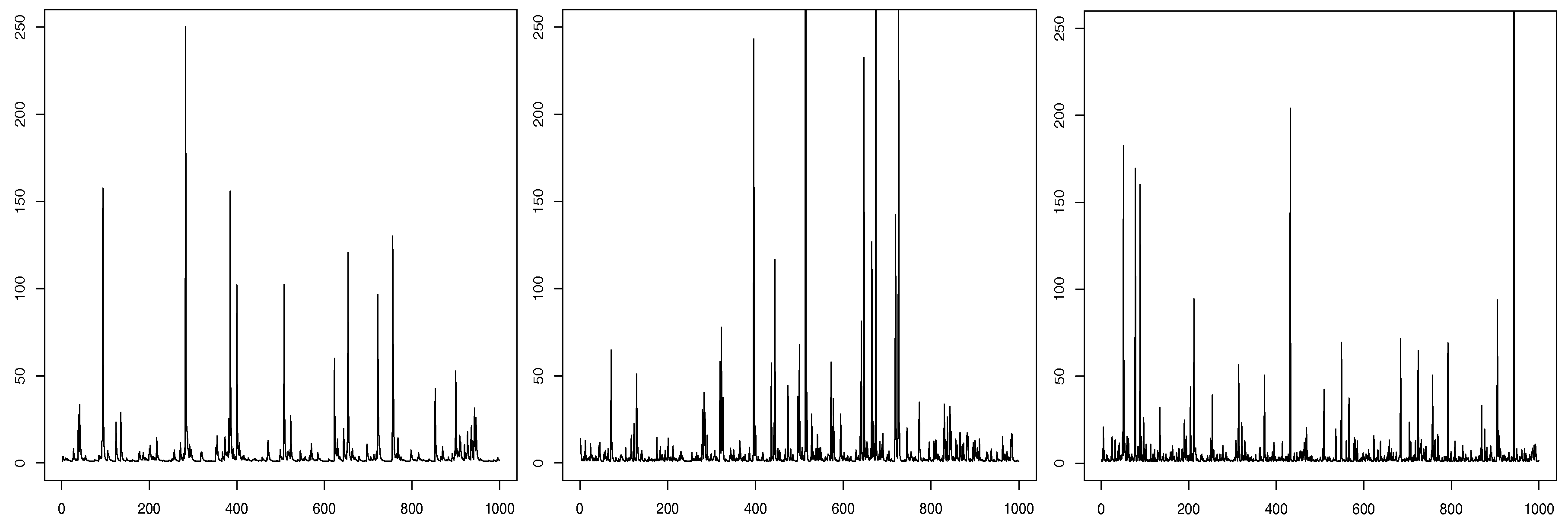
where ${\left\{{\mathsf{ϵ}}_n\right\}}_{n\ge 1}$ is an independent and identically distributed (iid) sequence with common df Pareto($\mathsf{\sigma },\mathsf{\alpha }$) given in Equation (1) and independent of the Bernoulli(p) iid sequence ${\left\{U_n\right\}}_{n\ge 1}$ with $0<p<1$, and ${\mathsf{ϵ}}_i$ independent of $X_j$ $\forall i>j$. If $X_0\sim$Pareto($\mathsf{\sigma },\mathsf{\alpha }$), then ${\left\{X_n\right\}}_{n\ge 1}$ is stationary also with marginal df Pareto($\mathsf{\sigma },\mathsf{\alpha }$). The GLP process corresponds to the exponentiated version of the Gaver–Lewis process introduced in Gaver and Lewis (1980), and hence its name. Simulated samples from the GLP process with marginals Pareto($1,1$) and $p=0.25,0.5,0.75$ are plotted in Figure 1.

This is a model within the heavy-tailed class where mean values (of different orders) may not exist. For instance, in this case, the mean exists only if $\mathsf{\alpha }>1$ and the variance/covariance exists whenever $\mathsf{\alpha }>2$. In Arnold (2001), the autocorrelation was derived as

$$\begin{array}{c}\hfill \mathsf{\rho }(X_{n-1},X_n)=\frac{(1-p)(\mathsf{\alpha }-2)}{\mathsf{\alpha }+p-2},\end{array}$$

(4)

for $\mathsf{\alpha }>2$. Moreover, in heavy-tailed models, the extremal observations are important, and a dependence analysis based on central measures like the most common autocorrelation may be misleading if the dependence in the tails presents a different structure from the remaining.

Here, we focus on the extremal behavior of the GLP process, namely the tail dependence structure. Despite being a heavy-tailed model, it is practically unknown in modeling extreme values. We shall see that it has interesting properties, such as asymptotic tail independence, i.e., the probability that one observation exceeds an increasing large value given that the previous one has already exceeded it, approaches zero. The rate of the convergence, usually denoted coefficient of asymptotic tail independence $\mathsf{\eta }$ (Ledford and Tawn (1996); Wadsworth and Tawn (2012)) captures a residual tail dependence, revealing a kind of “penultimate” clustering, i.e., an aggregation of not so high values. This is a not so fortuitous behavior in real applications and can be observed in the well-known Gaussian processes (see Bortot and Tawn (1998), Ramos and Ledford (2013), and references therein). In practice, ignoring this phenomena will result in misleading inference (see, e.g., Poon et al. (2003)). However, not all series associated with environmental, social or economic phenomena are susceptible to Gaussian modeling, especially when they have heavy tails. The most common extremal models MARMA and M4, as well as, the Yeh–Arnold–Robertson Pareto (III) and the Lawrence–Lewis Pareto processes (see, respectively, Ferreira (2012) and Ferreira (2016) and references therein) are not tail independent and new processes have been appearing (Heffernan et al. (2007); Ferreira and Canto e Castro (2010); Ferreira and Ferreira (2014) and Ferreira and Ferreira (2015) ). The GLP is an additional contribution within this class. Coefficient $\mathsf{\eta }$ will also be extended to observations that are lag-m apart, providing an alternative to the autocorrelation function (acf).

This paper is organized as follows. The tail dependence measures and conditions to be analyzed are detailed in Section 2 and applied to the GLP process in Section 3. The tail characterization provides us with methods to estimate the autoregressive parameter p, which will be compared through simulation in Section 4. An illustration with a real dataset is addressed in Section 5.

2. Tail Dependence

A stationary sequence ${\left\{X_n\right\}}_{n\ge 1}$ has extremal index $\mathsf{\theta }\in [0,1]$ if, for each $\mathsf{\tau }>0$, there is a sequence of normalized levels ${\{u_n\equiv u_n^{\left(\mathsf{\tau }\right)}\}}_{n\ge 1}$, i.e.,

$$\begin{array}{c}\hfill n(1-F\left(u_n\right))\to \mathsf{\tau },\end{array}$$

as $n\to \infty$, such that

$$\begin{array}{c}\hfill P(max(X_1,\cdots ,X_n)\le u_n)\to e^{-\mathsf{\theta }\mathsf{\tau }}\end{array}$$

(5)

(Leadbetter et al. (1983)). The extremal index is a measure for the clustering propensity, being interpreted as the arithmetic inverse of the mean number of exceedances of an increasing threshold per independent cluster. The null case is often ignored, corresponding to a degenerate limiting distribution for the maximum. The value $\mathsf{\theta }=1$ is associated to iid sequences but not only these. Below, we shall see that it is a form of asymptotic independence of extremes.

Some dependence conditions allow us to derive the extremal index through the joint distribution of s consecutive terms of ${\left\{X_n\right\}}_{n\ge 1}$.

The long-range condition D($u_n$) of Leadbetter (1974) states that ${\mathsf{\alpha }}_{n,l_n}\to 0$, as $n\to \infty$, for some sequence $l_n=o\left(n\right)$, where

$$\begin{array}{c}\hfill \begin{array}{cc}{\mathsf{\alpha }}_{n,l}=\hfill & sup\{|P\left(M_{i_1,i_1+p}\le u_n,M_{j_1,j_1+q}\le u_n\right)-P\left(M_{i_1,i_1+p}\le u_n\right)P\left(M_{j_1,j_1+q}\le u_n\right)|:\hfill \\ & 1\le i_1<i_1+p+l\le j_1<j_1+q\le n\},\hfill \end{array}\end{array}$$

(6)

with $M_{i,j}={max}_{s=i+1}^j\left(X_s\right)$, $M_{0,j}=M_j$ and $M_{i,j}=-\infty$ for $i\ge j$. Consider ${\left\{k_n\right\}}_{n\ge 1}$ such that,

$$\begin{array}{c}\hfill k_n\to \infty ,k_n{\mathsf{\alpha }}_{n,l_n}\to 0,k_n{l}_n/n\to 0,\mathrm{as}n\to \infty .\end{array}$$

(7)

Observe that D($u_n$) is a milder condition than the usual mixing, such as strong-mixing.

Under condition D($u_n$), we say that the local dependence condition D${}^{\left(s\right)}$($u_n$) of Chernick et al. (1991) holds for ${\left\{X_n\right\}}_{n\ge 1}$, if for some ${\left\{k_n\right\}}_{n\ge 1}$ satisfying Equation (7), we have

$$\begin{array}{c}\hfill {\displaystyle nP\left(X_1>u_n,M_{1,s}\le u_n<M_{s,r_n}\right)\underset{n\to \infty }{⟶}0,}\end{array}$$

with ${\{r_n=[n/k_n]\}}_{n\ge 1}$ ($\left[x\right]$ denoting the integer part of x). The validation of D${}^{\left(s\right)}$($u_n$) implies that D${}^{\left(s^{\prime }\right)}$($u_n$) holds for $s^{\prime }>s$.

If D${}^{\left(s\right)}$($u_n$) holds, the extremal index exists and can be computed through (Chernick et al. (1991))

$$\begin{array}{c}\hfill \mathsf{\theta }=\underset{n\to \infty }{lim}P(M_{1,s}\le u_n|X_1>u_n).\end{array}$$

(8)

Observe that, under D${}^{\left(1\right)}$($u_n$), we have $\mathsf{\theta }=1$. Condition D${}^{\left(s\right)}$($u_n$) is also implied by

$$\begin{array}{c}\hfill {\displaystyle n\sum _{j=s+1}^{r_n}P\left(X_1>u_n,M_{1,s}\le u_n<X_j\right)\underset{n\to \infty }{⟶}0.}\end{array}$$

This corresponds to condition D${}^{\prime }$($u_n$) of Leadbetter et al. (1983) whenever $s=1$, which locally restricts the occurrence of clusters of exceedances and thus leads to $\mathsf{\theta }=1$. Condition D${}^{″}$($u_n$) of Leadbetter and Nandagopalan (1989) is obtained with $s=2$ and locally restricts upcrossing clustering.

Observe that, under D${}^{″}$($u_n$), we can write

$$\begin{array}{c}\hfill \mathsf{\theta }=\underset{n\to \infty }{lim}P(X_2\le u_n|X_1>u_n)\end{array}$$

and thus state

$$\begin{array}{c}\hfill \mathsf{\theta }\left(u_n\right)\sim 1-P(X_2>u_n|X_1>u_n),n\to \infty ,\end{array}$$

where $a\left(x\right)\sim b\left(x\right)$ means $a\left(x\right)/b\left(x\right)\to c$, as $x\to \infty$, for some constant c. Observe that, if $\mathsf{\theta }<1$, then $P(X_2>u_n|X_1>u_n)>0$, meaning that consecutive observations are tail dependent. On the other hand, under a unit extremal index, we have $P(X_2>u_n|X_1>u_n)\to 0$, as $n\to \infty$, and thus consecutive observations are asymptotically tail independent. This feature has been observed in some real data and theoretical examples (Ledford and Tawn (1996); Bortot and Tawn (1998); Ramos and Ledford (2013)).

Ledford and Tawn (1996) introduced the asymptotic tail independence coefficient, $\mathsf{\eta }$, in order to measure the rate of convergence of $P(X_2>F^{-1}(1-t)|X_1>F^{-1}(1-t))$ towards 0, where $F^{-1}$ is the quantile function, capturing a kind of pre-asymptotic dependence. More precisely, the asymptotic tail independence coefficient, $\mathsf{\eta }\in [0,1]$, exists whenever it holds

$$\begin{array}{c}\hfill P\left(X_1>F^{-1}(1-t),X_2>F^{-1}(1-t)\right)\sim t^{1/\mathsf{\eta }}L(1/t),t\downarrow 0.\end{array}$$

(9)

Thus, under Equation (9), we can state,

$$\begin{array}{c}\hfill \mathsf{\theta }\left(u_n\right)\sim 1-P(X_2>u_n|X_1>u_n)\sim 1-u_n^{1-1/\mathsf{\eta }}L\left(u_n\right),n\to \infty .\end{array}$$

Observe that, if $\mathsf{\eta }=1$ and $L\left(u_n\right)\nrightarrow 0$, we have $\mathsf{\theta }<1$ and thus an effect of clustering of high values. Under a unit extremal index, the coefficient $\mathsf{\eta }<1$ measures the rate of convergence of $\mathsf{\theta }$ towards 1, capturing a kind of pre-asymptotic clustering, despite a resembling of the process to an iid sequence at increasingly high thresholds.

Analogous with the acf, we extend the coefficient $\mathsf{\eta }$ and state the tail dependence within random pairs that are lag-m apart, $(X_i,X_{i+m})$, $i\ge 1$, through the coefficient ${\mathsf{\eta }}_m$, i.e.,

$$P\left(X_1>F^{-1}(1-t),X_{1+m}>F^{-1}(1-t)\right)\sim t^{1/{\mathsf{\eta }}_m}L(1/t),t\downarrow 0,$$

where ${\mathsf{\eta }}_1\equiv \mathsf{\eta }$.

The tail dependent class has been greatly enhanced within the methodology of extreme values. However, this approach results in the overestimation of extremal dependence if the series is actually asymptotically independent. An illustration with financial data may be seen in Poon et al. (2003). The most recent literature has been addressing this issue, namely, with the introduction of new models comprising asymptotic tail independence (Heffernan et al. (2007); Ferreira and Canto e Castro (2010); (Ferreira and Ferreira) (2014, 2015). In the next section, we will show that the GLP belongs to this latter class of models.

3. The Tail Dependence of the Gaver–Lewis Process

In the following, and without loss of generality, we will take $\mathsf{\sigma }=1$.

“Mixing”conditions roughly state that two rvs become increasingly independent as they get more apart in time. One of its forms is the $\beta$-mixing condition, defined by

$$\begin{array}{c}\hfill {\displaystyle \mathsf{\beta }\left(l\right):=\underset{p\in \mathbb{N}}{sup}E\left(\underset{B\in \mathcal{F}(X_{p+l+1},...)}{sup}|P\left(B\right|\mathcal{F}(X_1,...,X_p))-P\left(B\right)|\right)\underset{l\to \infty }{⟶}0,}\end{array}$$

with $\mathcal{F}(.)$ denoting the $\mathsf{\sigma }-$field generated by the indicated random variables (Bradley (2005)).

Proposition 1.

The GLP process is $\mathsf{\beta }$-mixing.

Proof. 

The $\mathsf{\beta }$-mixing condition will be proved through the sufficient conditions of regeneration and aperiodicity (see, e.g., Bradley (2005); Corollary 3.6).

In the following, consider notation $Q^m(x,]1,y\left]\right)=P(X_{1+m}\le y|X_1=x)$, with $Q(x,]1,y\left]\right)\equiv Q^1(x,]1,y\left]\right)$.

Observe that

$$Q(x,]1,y\left]\right)=P(X_2\le y|X_1=x)=P\left({\mathsf{ϵ}}_2^{U_2}\le \frac{y}{x^{1-p}}\right)=F_{\mathsf{ϵ}}\left(\frac{y}{x^{1-p}}\right)p+1-p,y\ge x^{1-p}.$$

First, we show that GLP is regenerative, that is, it has a regeneration set, i.e., a recurrent set R such that, for some $m\in \mathbb{N}$, a distribution $\mathsf{\phi }$ and $\mathsf{\kappa }\in (0,1)$, we have

$$\begin{array}{c}\hfill Q^m(x,B)\ge \mathsf{\kappa }\mathsf{\phi }\left(B\right),x\in R\end{array}$$

for all Borel set B over $\mathbb{R}$. If, for any regeneration set R and any Borel set B over $\mathbb{R}$, we have

$$\begin{array}{c}\hfill Q^{m+1}(x,B)\ge {\mathsf{\kappa }}_1\phi \left(B\right)\mathrm{and}{Q}^m(x,B)\ge {\mathsf{\kappa }}_2\phi \left(B\right),\forall x\in R,\end{array}$$

(10)

for some $m\in \mathbb{N}$ and ${\mathsf{\kappa }}_1,{\mathsf{\kappa }}_2\in (0,1)$, then the process is said to be aperiodic (Asmussen (1987)).

Consider $R=]1,r[$ (and thus recurrent since it is in the state space $]1,\infty [$ of the process) and B a Borel set over $\mathbb{R}$. Let $x\in R$, $S=[r,r^{1/(1-p)}]$ and $V\sim$Pareto($r^{1-p},\mathsf{\alpha }$). For all $x\in R$, we have

$$Q(x,B)\ge {\int }_{B\cap S}dQ(x,z)\ge P(V\in B\cap S)p,$$

and thus regeneration holds by considering $m=1$, $\mathsf{\phi }\left(B\right)=P(V\in B|V\in S)$ and $\kappa =P(V\in S)p$. Observe that S is also regenerative since it is recurrent ($S\subset ]1,\infty [$) and, $\forall z\in S$, $z^{1-p}\le r<y$, for any $y\in S$, and thus $Q(z,B)\ge \kappa \mathsf{\phi }\left(B\right)$, with $\mathsf{\phi }\left(B\right)$ and $\mathsf{\kappa }$ as above. Now, we have

$$Q^2(x,B)\ge {\int }_{S}Q(z,B)dQ(x,z)\ge \mathsf{\kappa }\mathsf{\phi }\left(B\right)Q(x,S)\ge \mathsf{\kappa }\mathsf{\phi }\left(B\right)pP(V\in S).$$

Therefore, the aperiodicity condition in Equation (10) is satisfied if we take ${\mathsf{\kappa }}_1=\mathsf{\kappa }pP(V\in S)$ and ${\mathsf{\kappa }}_2=\mathsf{\kappa }$.  ☐

Note that condition $D\left(u_n\right)$ given in Equation (6) is weaker than $\mathsf{\beta }$-mixing and thus holds for GLP by the previous result.

Proposition 2.

The GLP process satisfies condition D${}^{\prime }$($u_n$) for sequences ${\left\{k_n\right\}}_{n\ge 1}$ satisfying Equation (7) and such that ${(2-p)}^{n/k_n}/n^p\to 0$, as $n\to \infty$.

Proof. 

We have successively, for $r_n=[n/k_n]$, $n\ge 1$,

$$\begin{array}{cc}& {\displaystyle n\sum _{j=2}^{r_n}P\left(X_1>u_n,X_j>u_n\right)}\hfill \\ \hfill =& {\displaystyle n\sum _{j=2}^{r_n}P\left(X_1>u_n,X_j>u_n,U_2=\dots =U_j=0\right)+n\sum _{j=2}^{r_n}\sum _{k=1}^{j-1}P\left(X_1>u_n,X_j>u_n,\sum _{i=2}^j{\mathbb{1}}_{\{U_i=1\}}=k\right)}\hfill \\ \hfill \le & {\displaystyle \sum _{j=2}^{r_n}\left(\frac{\mathsf{\tau }{(1-p)}^{j-1}}{{(n/\mathsf{\tau })}^{1/{(1-p)}^{j-1}-1}}+\sum _{k=1}^{j-1}\sum _{2\le s_1<\dots <s_k\le j}\frac{\mathsf{\tau }}{{(n/\mathsf{\tau })}^{1-{(1-p)}^{j-1}}}\prod _{\begin{array}{c}i=0\\ s_0=1\end{array}}^{k-1}\frac{p{(1-p)}^{j-1-k}}{1-{(1-p)}^{s_k-s_i}}\right)}\hfill \\ \hfill \le & {\displaystyle \sum _{j=2}^{r_n}\left(\frac{\mathsf{\tau }{(1-p)}^{j-1}}{{(n/\mathsf{\tau })}^{1/(1-p)-1}}+\sum _{k=1}^{j-1}\sum _{2\le s_1<\dots <s_k\le j}\frac{\mathsf{\tau }{(1-p)}^{j-1-k}}{{(n/\mathsf{\tau })}^p}\right)}\hfill \\ \hfill \le & {\displaystyle \frac{\mathsf{\tau }}{{(n/\mathsf{\tau })}^p}\sum _{j=2}^{r_n}\sum _{k=0}^{j-1}\left(\genfrac{}{}{0pt}{}{j-1}{k}\right){(1-p)}^{j-1-k}}\hfill \\ \hfill \le & {\displaystyle \frac{{\mathsf{\tau }}^{p+1}}{1-p}\frac{{(2-p)}^{r_n}}{n^p}.}\hfill \end{array}$$

(11)

☐

Corollary 1.

The GLP process has $\mathsf{\theta }=1$.

This result reveals that high observations of the GLP process behave similar to an iid scenario. However, there is a weak dependence that may be evaluated through the Ledford and Tawn coefficient $\mathsf{\eta }$ in Equation (9). Moreover, we will see that it relates with parameter p of the process.

Proposition 3.

The GLP process has $\mathsf{\eta }=1/(1+p)$.

Proof. 

Consider $a_t=F_X^{-1}(1-t)$ and take $t\downarrow 0$. Observe that

$$\begin{array}{cc}& {\displaystyle P\left(X_1>a_t,X_2>a_t\right)}\hfill \\ \hfill =& pP(X_1>a_t,X_1^{1-p}{\mathsf{ϵ}}_2>a_t)+(1-p)P(X_1>a_t,X_1^{1-p}>a_t)\hfill \\ \hfill =& {\displaystyle p{\int }_{a_t}^{\infty }{\overline{F}}_{{\mathsf{ϵ}}_2}(a_t/x^{1-p})d{F}_X\left(x\right)+(1-p){\overline{F}}_X\left(a_t^{1/(1-p)}\right)}\hfill \\ \hfill =& a_t^{-\mathsf{\alpha }(1+p)}+(1-p)a_t^{-\mathsf{\alpha }/(1-p)}\sim t^{p+1}+t^{1/(1-p)}(1-p),\mathrm{as}n\to \infty .\hfill \end{array}$$

☐

The fluctuation probability in the GLP process, given by

$$\begin{array}{c}\hfill \begin{array}{cc}\hfill f:=& {\displaystyle P(X_{n-1}<X_n)=pP(X_{n-1}^p<{\mathsf{ϵ}}_n)=p{\int }_1^{\infty }{F}_X\left(x^{1/p}\right)d{F}_{\mathsf{ϵ}}\left(x\right)=p/(1+p),}\hfill \end{array}\end{array}$$

is a simple measure that will be useful in the following.

Corollary 2.

The GLP process verifies the following equalities:

• (i) $p=1/(1-f)-1$;
• (ii) $p=1/\eta -1$;
• (iii) $\eta =1-f$.

This result states a characterizing feature that can be helpful in model specification. Moreover, in order to satisfy $0<p<1$, we must have $0<f<1/2$ and $1/2<\eta <1$.

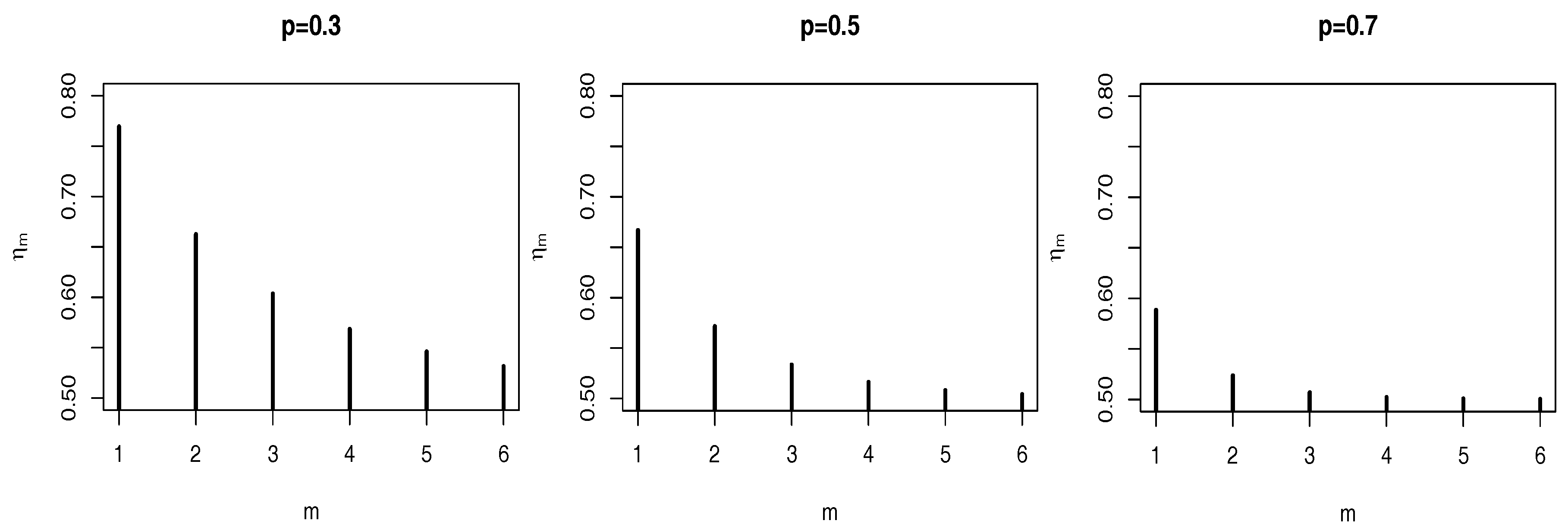
Another interesting property for model identification is based on the lag-m coefficient ${\mathsf{\eta }}_m$, analogous with the acf for linear models. The plots in Figure 2 exhibit a power decay as the acf of AR(1) processes. Observe also that the smaller the value of p, the higher we must choose the lag-m in order to have "almost" independent observations, i.e., ${\mathsf{\eta }}_m\approx 1/2$.

Proposition 4.

The GLP process has lag-m coefficient ${\eta }_m$ given by

$$\begin{array}{c}\hfill {\mathsf{\eta }}_m=1/\left(2-{(1-p)}^m\right).\end{array}$$

(12)

Proof. 

Consider $a_t=F_X^{-1}(1-t)$. The product of powered Pareto rvs is still Pareto-type tail distributed (see, e.g., Arnold (2001)) and thus, applying Equation (2) and the theorem of the dominated convergence, we have successively, as $t\downarrow 0$,

$$\begin{array}{cc}& {\displaystyle P\left(X_1>a_t,X_{1+m}>a_t\right)={\int }_{a_t}^{\infty }P\left(x^{{(1-p)}^m}\prod _{j=0}^{m-1}{\mathsf{ϵ}}_{m+1-j}^{U_{m+1-j}{(1-p)}^j}>a_t\right)d{F}_X\left(x\right)}\hfill \\ \hfill \sim & {\displaystyle {\int }_{a_t}^{a_t^{{(1-p)}^{-(m+1)}}}{\left(a_t{x}^{-{(1-p)}^{m+1}}\right)}^{-\mathsf{\alpha }}L(x/t)d{F}_X\left(x\right)+{\int }_{a_t^{{(1-p)}^{-(m+1)}}}^{\infty }d{F}_X\left(x\right)}\hfill \\ \hfill \sim & {\displaystyle a_t^{-\mathsf{\alpha }}L(1/t){\int }_{a_t}^{a_t^{{(1-p)}^{-(m+1)}}}\mathsf{\alpha }{x}^{-\mathsf{\alpha }(1-{(1-p)}^{m+1})-1}dx+a_t^{-\mathsf{\alpha }{(1-p)}^{-(m+1)}}}\hfill \\ \hfill =& {\displaystyle \frac{a_t^{-\mathsf{\alpha }}L(1/t)}{1-{(1-p)}^{m+1}}\left(a_t^{-\mathsf{\alpha }(1-{(1-p)}^{m+1})}-a_t^{-\mathsf{\alpha }({(1-p)}^{-(m+1)}-1)}\right)+a_t^{-\mathsf{\alpha }{(1-p)}^{-(m+1)}}}\hfill \\ \hfill \sim & {\displaystyle L^{\ast }(1/t)\left(t^{2-{(1-p)}^{m+1}}\right),}\hfill \end{array}$$

(13)

where $L(1/t)$ and $L^{\ast }(1/t)$ are slowly varying functions.  ☐

4. Estimation

Relations (i) and (ii) stated in Corollary 2 will provide us with estimators for the autoregressive parameter p. More precisely, from (i), we have

$$\begin{array}{c}\hfill {\widehat{p}}^{\left(F\right)}=\frac{1}{1-\widehat{f}}-1,\end{array}$$

(14)

with $\widehat{f}$ corresponding to the empirical counterpart of f,

$$\begin{array}{c}\hfill \widehat{f}=\frac{1}{n-1}\sum _{j=2}^n{\mathrm{𝟙}}_{\{X_{j-1}<X_j\}},\end{array}$$

provided that $\widehat{f}<1/2$ (notation ${\mathrm{𝟙}}_{\{·\}}$ means the indicator function). From the iid property of the generating process ${\epsilon }_t$ (and with $X_0$ as specified for stationarity), we have ergodicity and thus consistence of the proposed estimators. In addition, $\widehat{f}$ corresponds to the mean of Bernoulli trials with Markov dependence. From Klotz (1973), we have that $\sqrt{n}(\widehat{f}-f)$ converges in distribution to a centered Gaussian model, and thus $\sqrt{n}({\widehat{p}}^{\left(F\right)}-p)$ by the Delta Method, as $n\to \infty$. For more details, see Ferreira (2012).

From (ii), the estimation of p is based on the estimation of $\eta$ through

$$\begin{array}{c}\hfill {\widehat{p}}^{\left(H\right)}=\frac{1}{{\widehat{\mathsf{\eta }}}^{\left(H\right)}}-1,\end{array}$$

(15)

as long as ${\widehat{\mathsf{\eta }}}^{\left(H\right)}>1/2$. Observe that $\mathsf{\eta }$ corresponds to the tail index of $T=min(1/(1-F\left(X_1\right)),1/(1-F\left(X_2\right)))$. The most common method developed in literature is the Hill estimator (Hill (1975))—thus the superscript “H”. More precisely, we have

$$\begin{array}{c}\hfill {\widehat{\mathsf{\eta }}}^{\left(H\right)}=\frac{1}{k}\sum _{i=1}^{k}log{T}_{n-i+1:n}-logu,\end{array}$$

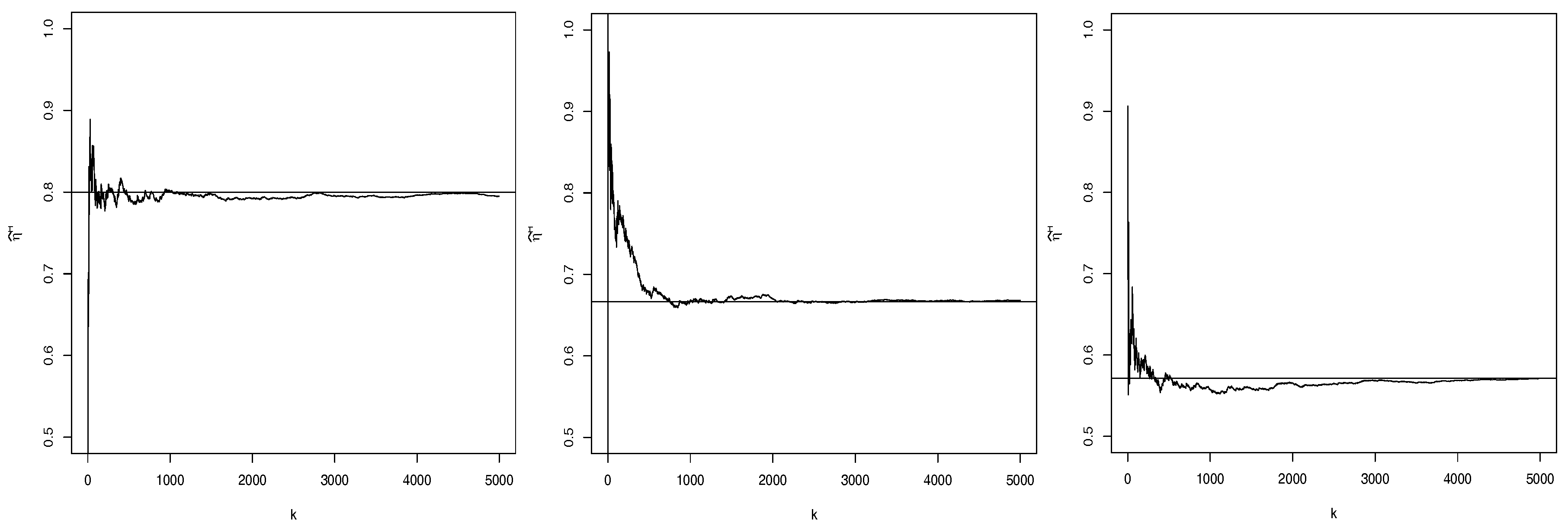
where $T_{n-k+1:n},\cdots ,T_{n:n}$ are the k larger order statistics of T that exceed u. It is usual to consider $u\in [T_{n-k:n},T_{n-k+1:n}[$ and plot ${\widehat{\mathsf{\eta }}}^{\left(H\right)}$ as a function of k. In Figure 3, we can see the Hill trajectories of $\widehat{\mathsf{\eta }}$ for the respective GLP models considered in Figure 1. The paths are quite stable around the true value of $\mathsf{\eta }$ for a large range of values of k. Indeed, variable T corresponds to the minimum of unit Pareto rvs, where the Hill estimator behaves particularly well. Consistency and asymptotic normality of the Hill estimator ${\widehat{\mathsf{\eta }}}^{\left(H\right)}$ can be seen in Draisma et al. (2004).

Expecting to observe time series data behaving exactly as the GLP functional Equation (3) is not realistic. At best, we might observe perturbed versions of the GLP process, for instance “noisy” processes of the form $X_n^{\left(\mathsf{\delta }\right)}=X_n+\mathsf{\delta }{Z}_n$, $n\ge 1$, where ${\left\{Z_n\right\}}_{n\ge 1}$ is an iid sequence of standard Gaussian rvs and $\mathsf{\delta }>0$. Thus, the simulations cover the GLP and “noisy” GLP sample paths for $\mathsf{\delta }=0,0.1,1$. We consider 1000 replicas of sizes $n=100,1000,5000$ for $p=0.25,0.5,0.75$, and marginals Pareto($1,1$). The computed estimates of the root mean squared error (rmse) and absolute bias (abias) are reported in

Table 1. Simulation results of the root mean squared error (RMSE) and of the absolute bias (abias). The last three columns correspond to the number of fails (nf) in each case.

			RMSE			abias
$n=100$		$\mathsf{\delta }=0$	$\mathsf{\delta }=0.1$	$\mathsf{\delta }=1$	$\mathsf{\delta }=0$	$\mathsf{\delta }=0.1$	$\mathsf{\delta }=1$	$n{f}_{\mathsf{\delta }=0}$	$n{f}_{\mathsf{\delta }=0.1}$	$n{f}_{\mathsf{\delta }=1}$
$p=0.25$	${\widehat{p}}^{\left(F\right)}$	0.0548	0.1844	0.5050	0.0005	0.1693	0.4940	0	0	24
	${\widehat{p}}_{q_0}^{\left(H\right)}$	0.0775	0.0837	0.2302	0.0547	0.0070	0.2127	0	0	1
	${\widehat{p}}_{q_{50}}^{\left(H\right)}$	0.1225	0.1140	0.1095	0.0801	0.0130	0.0202	0	0	1
	${\widehat{p}}_{q_{80}}^{\left(H\right)}$	0.2280	0.2236	0.2098	0.1587	0.0500	0.0842	8	7	35
$p=0.5$	${\widehat{p}}^{\left(F\right)}$	0.0707	0.1225	0.3317	0.0013	0.0943	0.3200	0	0	68
	${\widehat{p}}_{q_0}^{\left(H\right)}$	0.0894	0.0894	0.1789	0.0492	0.0557	0.1576	0	0	0
	${\widehat{p}}_{q_{50}}^{\left(H\right)}$	0.1342	0.1414	0.1342	0.0586	0.0633	0.0197	2	2	1
	${\widehat{p}}_{q_{80}}^{\left(H\right)}$	0.2191	0.2121	0.2049	0.0816	0.0783	0.0182	100	83	68
$p=0.75$	${\widehat{p}}^{\left(F\right)}$	0.0894	0.0548	0.1483	0.0001	0.0265	0.1287	10	0	222
	${\widehat{p}}_{q_0}^{\left(H\right)}$	0.1000	0.0949	0.1265	0.0419	0.0422	0.0917	21	22	93
	${\widehat{p}}_{q_{50}}^{\left(H\right)}$	0.1265	0.1225	0.1342	0.0116	0.0120	0.0028	143	123	121
	${\widehat{p}}_{q_{80}}^{\left(H\right)}$	0.1975	0.1897	0.1975	0.0611	0.0526	0.0686	311	274	267
$n=1000$	rmse	$\delta$ = 0	$\delta$ = 0.1	$\delta$ = 1	$\delta$ = 0	$\delta$ = 0.1	$\delta$ = 1	nf${}_{\delta =0}$	nf${}_{\delta =0.1}$	nf${}_{\delta =1}$
$p=0.25$	${\widehat{p}}^{\left(F\right)}$	0.0000	0.1673	0.5010	0.0003	0.1656	0.4998	0	0	0
	${\widehat{p}}_{q_0}^{\left(H\right)}$	0.0775	0.0000	0.1449	0.0547	0.0169	0.1423	0	0	0
	${\widehat{p}}_{q_{50}}^{\left(H\right)}$	0.1225	0.0316	0.0775	0.0801	0.0080	0.0742	0	0	0
	${\widehat{p}}_{q_{80}}^{\left(H\right)}$	0.2280	0.0548	0.0775	0.1587	0.0209	0.0494	8	0	0
$p=0.5$	${\widehat{p}}^{\left(F\right)}$	0.0000	0.0949	0.3302	0.0005	0.0943	0.3285	0	0	0
	${\widehat{p}}_{q_0}^{\left(H\right)}$	0.0316	0.0316	0.1095	0.0058	0.0122	0.1068	0	0	0
	${\widehat{p}}_{q_{50}}^{\left(H\right)}$	0.0447	0.0447	0.0632	0.0087	0.0072	0.0508	0	0	0
	${\widehat{p}}_{q_{80}}^{\left(H\right)}$	0.0775	0.0775	0.0949	0.0158	0.0143	0.0459	0	0	0
$p=0.75$	${\widehat{p}}^{\left(F\right)}$	0.0316	0.0548	0.1732	0.0006	0.0459	0.1695	0	0	10
	${\widehat{p}}_{q_0}^{\left(H\right)}$	0.0316	0.0316	0.0707	0.0053	0.0075	0.0636	0	0	0
	${\widehat{p}}_{q_{50}}^{\left(H\right)}$	0.0548	0.0548	0.0548	0.0084	0.0062	0.0186	0	0	0
	${\widehat{p}}_{q_{80}}^{\left(H\right)}$	0.1000	0.0949	0.1000	0.0120	0.0047	0.0287	16	16	7
$n=5000$	rmse	$\delta$ = 0	$\delta$ = 0.1	$\delta$ = 1	$\delta$ = 0	$\delta$ = 0.1	$\delta$ = 1	nf${}_{\delta =0}$	nf${}_{\delta =0.1}$	nf${}_{\delta =1}$
$p=0.25$	${\widehat{p}}^{\left(F\right)}$	0.0000	0.1643	0.5000	0.0002	0.1649	0.4994	0	0	0
	${\widehat{p}}_{q_0}^{\left(H\right)}$	0.0000	0.0000	0.1378	0.0015	0.0107	0.1360	0	0	0
	${\widehat{p}}_{q_{50}}^{\left(H\right)}$	0.0000	0.0000	0.0837	0.0027	0.0004	0.0836	0	0	0
	${\widehat{p}}_{q_{80}}^{\left(H\right)}$	0.0316	0.0316	0.0707	0.0054	0.0044	0.0618	0	0	0
$p=0.5$	${\widehat{p}}^{\left(F\right)}$	0.0000	0.0949	0.3302	0.0002	0.0939	0.3302	0	0	0
	${\widehat{p}}_{q_0}^{\left(H\right)}$	0.0000	0.0000	0.1049	0.0004	0.0061	0.1025	0	0	0
	${\widehat{p}}_{q_{50}}^{\left(H\right)}$	0.0000	0.0000	0.0632	0.0007	0.0004	0.0567	0	0	0
	${\widehat{p}}_{q_{80}}^{\left(H\right)}$	0.0316	0.0316	0.0632	0.0020	0.0021	0.0563	0	0	0
$p=0.75$	${\widehat{p}}^{\left(F\right)}$	0.0000	0.0447	0.1703	0.0002	0.0451	0.1685	0	0	0
	${\widehat{p}}_{q_0}^{\left(H\right)}$	0.0000	0.0000	0.0632	0.0011	0.0034	0.0585	0	0	0
	${\widehat{p}}_{q_{50}}^{\left(H\right)}$	0.0316	0.0316	0.0316	0.0013	0.0000	0.0257	0	0	0
	${\widehat{p}}_{q_{80}}^{\left(H\right)}$	0.0447	0.0447	0.0548	0.0037	0.0026	0.0367	0	0	0

, where the estimator ${\widehat{p}}^{\left(H\right)}$ is based on thresholds u corresponding to the sample minimum ($q_0$), the median ($q_{50}$) and the percentile 80 ($q_{80}$). We also register the number of fails resulting, respectively, from $\widehat{f}\ge 1/2$ and ${\widehat{\mathsf{\eta }}}^{\left(H\right)}\le 1/2$. Not surprisingly, they are more associated to small sample sizes, where the case $p=0.75$ seems particularly sensitive. Indeed, the results tend to be slightly worse under large $p=0.75$, where the process approximates to independence. In practice, the difficulty in deciding between tail dependence ($\mathsf{\eta }=1$) and asymptotic independence ($\mathsf{\eta }<1$) is well known. For a survey on this topic, see, e.g., Poon et al. (2003) and Beirlant et al. (2004). The results get better as the sample sizes increase. We observe that estimator ${\widehat{p}}^{\left(F\right)}$ is the best for the GLP process but not so robust for “noisy” GLP. In what concerns estimator ${\widehat{p}}^{\left(H\right)}$, it seems to present an overall better performance under $u=q_0$.

The estimation of the tail index parameter $\mathsf{\alpha }$ may be conducted through the Hill estimator ${\widehat{\mathsf{\alpha }}}^{\left(H\right)}$ (Hill (1975)), which is consistent and asymptotically normal under strong mixing conditions (see Rootzn et al. (1990)).

5. Application

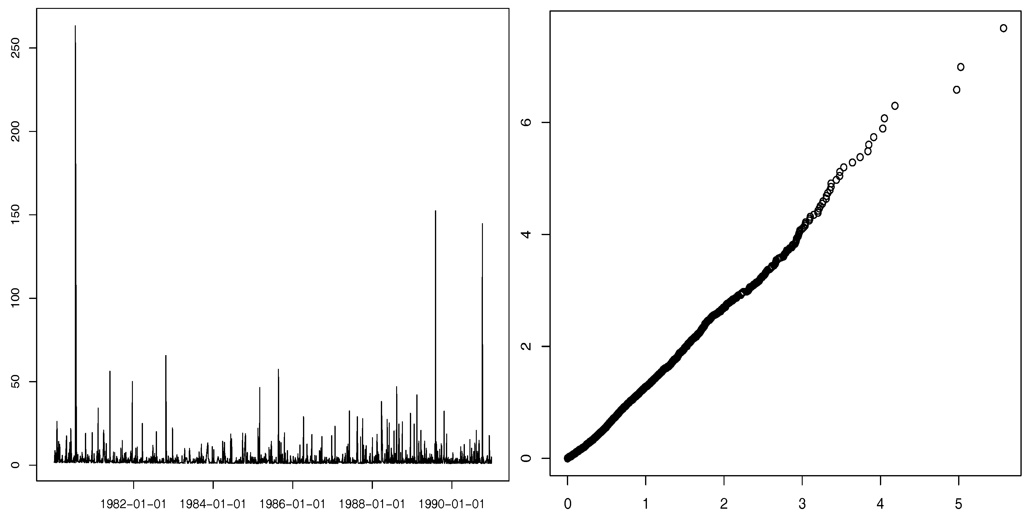
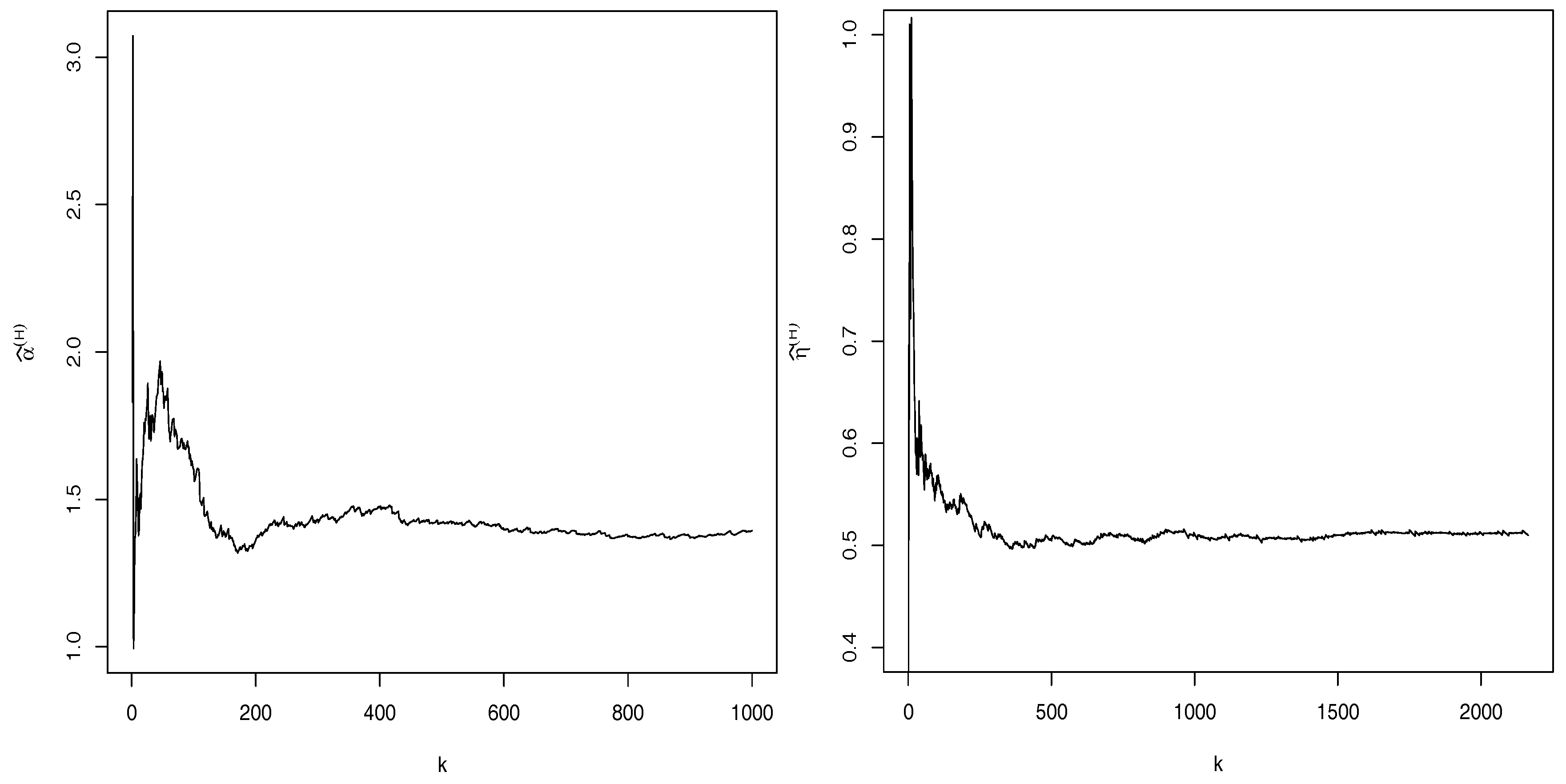
Insurance loss data is typically well modeled by heavy-tailed processes. We consider the daily closing values for the Danish fire losses registered from January 1980 to December 1990, plotted in Figure 4 (left). Observe the high values that appear suddenly, similar to the GLP simulated sample paths (see Figure 1), as well as the close linearity of the Pareto quantile-quantile plot (right panel of Figure 4). In Figure 5 (left), the almost plane region of Hill’s sample path led us to the estimate ${\widehat{\mathsf{\alpha }}}^{\left(H\right)}\approx 1.4$. Thus, we cannot assume the existence of the acf and should avoid an analysis based on this tool. We conduct the estimate of the GLP parameter p through ${\widehat{p}}^{\left(F\right)}$ and ${\widehat{p}}^{\left(H\right)}$. More precisely, based on Equation (14), we obtain ${\widehat{p}}^{\left(F\right)}=0.9945$ and, using Equation (15), we derive ${\widehat{p}}_{q_0}^{\left(H\right)}=0.9610$, ${\widehat{p}}_{q_{50}}^{\left(H\right)}=0.9715$ and ${\widehat{p}}_{q_{80}}^{\left(H\right)}=0.9996$, where the quantiles $q_0$, $q_{50}$ and $q_{80}$ were considered according to the simulation study (see also the sample path estimates of Hill in the right panel of Figure 5). Formula (12) of the lag-m coefficient ${\mathsf{\eta }}_m$ of Proposition 4 is a similar tool to the role of the acf in identifying linear models.

Table 2. Danish fire losses: estimates of the lag-m coefficient ${\mathsf{\eta }}_m$.

${\widehat{\mathsf{\eta }}}_1({\widehat{p}}^{\left(F\right)})$		0.5014
${\widehat{\mathsf{\eta }}}_2({\widehat{p}}^{\left(F\right)})$		0.5000
${\widehat{\mathsf{\eta }}}_3({\widehat{p}}^{\left(F\right)})$		0.5000
$\widehat{{\mathsf{\eta }}_m}$	$q_0$	$q_{50}$	$q_{80}$
${\widehat{{\mathsf{\eta }}_1}}^{\left(H\right)}\equiv {\widehat{\mathsf{\eta }}}_1({\widehat{p}}^{\left(H\right)})$	0.5099	0.5072	0.5001
${\widehat{{\mathsf{\eta }}_2}}^{\left(H\right)}$	0.5094	0.4995	0.5209
${\widehat{\mathsf{\eta }}}_2({\widehat{p}}^{\left(H\right)})$	0.5004	0.5002	0.5000
${\widehat{{\mathsf{\eta }}_3}}^{\left(H\right)}$	0.5081	0.4985	0.4820
${\widehat{\mathsf{\eta }}}_3({\widehat{p}}^{\left(H\right)})$	0.5000	0.5000	0.5000

presents the estimates of ${\mathsf{\eta }}_m$, for $m=1,2,3$, obtained from estimator ${\widehat{\mathsf{\eta }}}_m^{\left(H\right)}$, which consists of the Hill estimator, respectively applied to lag-m apart random pairs $(X_i,X_{i+m})$, as well as, estimates of ${\widehat{\mathsf{\eta }}}_m({\widehat{p}}^{\left(F\right)})$ and ${\widehat{\mathsf{\eta }}}_m({\widehat{p}}^{\left(H\right)})$ derived from Equation (12) by replacing p, respectively, by ${\widehat{p}}^{\left(F\right)}$ and ${\widehat{p}}^{\left(H\right)}$. The closeness between the two type of estimates, ${\widehat{\mathsf{\eta }}}_m^{\left(H\right)}$ and ${\widehat{\mathsf{\eta }}}_m({\widehat{p}}^{(·)})$, shows a further contribution in favor of the model.

The GLP process thus seems to have potential in the modeling of this type of data. More tools regarding goodness-of-fit analysis will be addressed in a future work.

References

1. Arnold, Barry C. 2001. Pareto Processes. In Handbook of Statistics. Edited by D. N. Shanbhag and C. R. Rao. Vol. 19, Amsterdam: Elsevier Science B.V. [Google Scholar]
2. Asmussen, Soren. 1987. Applied Probability and Queues. Hoboken: John Wiley & Sons. [Google Scholar]
3. Beirlant, Jan, Yuri Goegebeur, Johan Segers, and Jozef Teugels. 2004. Statistics of Extremes: Theory and Applications. Hoboken: John Wiley & Sons. [Google Scholar]
4. Bortot, Paola, and Jonathan A. Tawn. 1998. Models for the extremes of Markov chains. Biometrika 85: 851–67. [Google Scholar] [CrossRef]
5. Bradley, Richard C. 2005. Basic Properties of Strong Mixing Conditions. A Survey and Some Open Questions. Probability Surveys 2: 107–44. [Google Scholar] [CrossRef]
6. Chernick, Michael R., Tailen Hsing, and William P. McCormick. 1991. Calculating the extremal index for a class of stationary sequences. Advance in Appliec Probability 23: 835–50. [Google Scholar] [CrossRef]
7. Davis, Richard A., and Sidney I. Resnick. 1989. Basic properties and prediction of max-ARMA processes. Advance in Appliec Probability 21: 781–803. [Google Scholar] [CrossRef]
8. Draisma, Draisma, Holger Dress, Ana Ferreira, and Laurens de Haan. 2004. Bivariate tail estimation: dependence in asymptotic independence. Bernoulli 10: 251–80. [Google Scholar] [CrossRef]
9. Ferreira, Marta. 2016. The Lawrence-Lewis Pareto process: an extremal approach. Electronic Journal of Applied Statistical Analysis 9: 68–82. [Google Scholar]
10. Ferreira, Marta. 2012. On the extremal behavior of a Pareto process: An alternative for armax modeling. Kybernetika 48: 31–49. [Google Scholar]
11. Ferreira, Marta, and Luísa Canto e Castro. 2010. Modeling rare events through a pRARMAX process. Journal of Statistical Planning and Inference 140: 3552–66. [Google Scholar] [CrossRef]
12. Ferreira, Helena, and Marta Ferreira. 2015. Extremes of scale mixtures of multivariate time series. Journal of Multivariate Analysis 137: 82–99. [Google Scholar] [CrossRef]
13. Ferreira, Helena, and Marta Ferreira. 2014. Extremal behavior of pMAX processes. Statistics & Probability Letters 93: 46–57. [Google Scholar]
14. Gaver, Donald, and P. A. W. Lewis. 1980. First-Order Autoregressive Gamma Sequences and Point Processes. Advances in Applied Probability 12: 727–45. [Google Scholar] [CrossRef]
15. Heffernan, Janet E., Jonathan A. Tawn, and Zhengjun Zhang. 2007. Asymptotically (in)dependent multivariate maxima of moving maxima processes. Extremes 10: 57–82. [Google Scholar] [CrossRef]
16. Hill, Bruce M. 1975. A Simple General Approach to Inference About the Tail of a Distribution. The Annals of Statistics 3: 1163–74. [Google Scholar] [CrossRef]
17. Klotz, Jerome. 1973. Statistical inference in Bernoulli trials with dependence. The Annals of Statistics 1: 373–79. [Google Scholar] [CrossRef]
18. Leadbetter, M. Ross. 1974. On extreme values in stationary sequences. Zeitschrift Für Wahrscheinlichkeitstheorie Und Verwandte Gebiete 28: 289–303. [Google Scholar] [CrossRef]
19. Leadbetter, Malcolm R., Georg Lindgren, and Holger Rootzén. 1983. Extremes and Related Properties of Random Sequences and Processes. New York: Springer. [Google Scholar]
20. Leadbetter, M. Ross, and S. Nandagopalan. 1989. On exceedance point processes for stationary sequences under mild oscillation restrictions. Lecture Notes in Statistics 51: 69–80. [Google Scholar]
21. Ledford, Anthony W., and Jonathan A. Tawn. 1996. Statistics for near independence in multivariate extreme values. Biometrika 83: 169–87. [Google Scholar] [CrossRef]
22. Poon, Ser-Huang, Michael Rockinger, and Jonathan Tawn. 2003. Modelling Extreme-Value Dependence in International Stock Markets. Statistica Sinica 13: 929–53. [Google Scholar] [CrossRef]
23. Ramos, Alexandra, and Anthony Ledford. 2013. Estimation of the extremal index function in case of asymptotically independent Markov chains and its application to stock market indexes. In Studies in Theoretical and Applied Statistics: Subseries B: Recent Developments in Modeling and Applications in Statistics (SPE2010). Edited by P. Oliveira, M. G. Temido, C. Henriques and M. Vichi. New York: Springer, pp. 89–96. [Google Scholar]
24. Rootzen, Holger, Malcolm R. Leadbetter, and Laurens De Haan. 1990. Tail and Quantile Estimation for Strongly Mixing Stationary Sequences. Series: Report 9024/A; Rotterdam: Erasmus University. [Google Scholar]
25. Smith, Richard L., and Ishay Weissman. 1996. Characterization and Estimation of the Multivariate Extremal Index. Technical Report. Chapel Hill: Universityof North Carolina. [Google Scholar]
26. Wadsworth, Jennifer L., and Jonathan A. Tawn. 2012. Dependence modelling for spatial extremes. Biometrika 99: 253–72. [Google Scholar] [CrossRef]
Figure 1. Simulated sample paths of the GLP process with marginals Pareto( 1 , 1 ) for p = 0.25 (left), p = 0.5 (middle) and p = 0.75 (right).
Risks 05 00033 g001
Figure 2. Plots of η m for the GLP process with p = 0.3 (left); p = 0.5 (middle) and p = 0.7 (right), for lags m = 1 , , 6 .
Risks 05 00033 g002
Figure 3. Hill plots of η ^ ( H ) for the GLP process with marginals Pareto( 1 , 1 ) and p = 0.25 (left); p = 0.5 (middle) and p = 0.75 (right).
Risks 05 00033 g003
Figure 4. Danish fire losses: daily closing values from January 1980 to December 1990 (left); Pareto quantile-quantile plot (right).
Risks 05 00033 g004
Figure 5. Danish fire losses: trajectory of Hill estimates of α ^ ( H ) (left) and η ^ ( H ) (right).
Risks 05 00033 g005