Best-Estimates in Bond Markets with Reinvestment Risk

Abstract

The concept of best-estimate, prescribed by regulators to value insurance liabilities for accounting and solvency purposes, has recently been discussed extensively in the industry and related academic literature. To differentiate hedgeable and non-hedgeable risks in a general case, recent literature defines best-estimates using orthogonal projections of a claim on the space of replicable payoffs. In this paper, we apply this concept of best-estimate to long-maturity claims in a market with reinvestment risk, since in this case the total liability cannot easily be separated into hedgeable and non-hedgeable parts. We assume that a limited number of short-maturity bonds are traded, and derive the best-estimate price of bonds with longer maturities, thus obtaining a best-estimate yield curve. We therefore use the multifactor Vasiček model and derive within this framework closed-form expressions for the best-estimate prices of long-term bonds.

1. Introduction

Life insurers are often faced with the problem of valuing liabilities with long maturities. While the market for long-term bonds is rarely liquid, insurers regularly need to value liabilities with terms over 30 years. Under the new solvency regulations, in which liabilities must be valued on a “mark-to-market” approach, such maturities can pose a challenge for insurers. In fact, the market consistency prescribed by regulators dictates that hedgeable risks (the part of financial obligations that can be replicated by admissible traded assets) be valued using the market prices of their traded counterparts. To be admissible, the assets must be traded on a deep, liquid and transparent market, which is not the case for bonds with long maturities (see Wüthrich [1] for more details). Further techniques are thus needed to value long-term insurance liabilities for accounting and solvency purposes.

When liabilities cannot be marked to market, a popular approach is to “mark-to-model”, that is, to fit a model using information available in active markets and to use this model to price the liabilities (see, for example, Bierbaum et al. [2] and Martin [3]). This approach disregards the impossibility to completely hedge long-term payoffs, even deterministic ones, using only the short- and medium-term bonds traded in active markets. In such cases, the hedging portfolio must be readjusted as short-term bonds reach maturity and new bonds become available. This strategy involves reinvestment risk, which should be reflected in the value of the long-term liabilities. An introduction to reinvestment risk in the context of long-term contracts is given in Dahl [4]. Stefanovits-Wüthrich [5] present a method to hedge and value long-term zero-coupon bonds with reinvestment risk by extrapolating the yield curve for different risk tolerance levels. In this paper, we attempt to calculate the best-estimate price of a long term zero-coupon bond in a market with reinvestment risk, where “best-estimate” is as prescribed by Solvency II regulations.

In a recent work, Happ et al. [6] provide a rigorous definition of best-estimate insurance reserves in a multiperiod discrete time financial market setting. Under this interpretation of the Solvency II Framework Directive [7], best-estimate reserves are obtained as follows: insurance risks that can be separated (independently) into a hedgeable part using market traded admissible assets and a (orthogonal) non-hedgeable part should be valued at the market price of the resulting portfolio of these traded instruments. In simple cases, the two types of risk can be separated using conditional expectations, as explained in Section 4.1 of [6]. However, when this separation is not possible, the authors conclude that the sequential local risk-minimization approach of Föllmer-Schweizer [8] and Malamud et al. [9,10] is an appropriate and consistent approach in the Solvency II framework. They show that this approach corresponds to the recursive application of orthogonal projections onto the space of one-period replicable payoffs. Since there might not exist an equivalent risk-neutral measure under which this best-estimate price can be calculated, appropriate state-price deflators are used and expectations are taken under the real-world (objective) measure.

The best-estimate definition given by [6] was developed for a general financial model. In this paper, we apply their definition of best-estimate reserves to value zero-coupon bonds with long maturities in financial markets with reinvestment risk, whose hedgeable part cannot be separated by a conditional expectation. In our market, reinvestment risk stems from the fact that only a limited number of bonds are available on the market. In this context, we value a zero-coupon bond with time to maturity longer than the longest traded bond. The best-estimate thus obtained takes into account the lack of liquidity on the long-maturity bond market. To analyse this valuation method we use the multifactor Vasiček model since it provides a flexible modeling framework with tractable formulas for the valuation of long-term bonds. We remark at this stage that this choice was mainly motivated by tractability, and similar studies should also be conducted for other term structure models. Using numerical examples, we show that the number of bonds available and the correlation structure between the bond prices influence the best-estimate price of the long-maturity bond.

The paper is organized as follows. In Section 2, we present the bond market with reinvestment risk and recall the definition of best-estimates presented by [6]. In Section 3, we derive expressions for best-estimate bond prices in the Vasiček model. Numerical illustrations are presented in Section 4 and Section 5 concludes. Proofs are provided in the Appendix.

2. Bond Market with Reinvestment Risk

We begin by introducing the setting considered in [6] and we adapt it to model a bond market with reinvestment risk. Fix a finite time horizon $n\in \mathbb{N}$ and consider a filtered probability space $(\mathrm{\Omega },𝓕,\mathbb{P},𝔽)$ where $\mathbb{P}$ is the real-world probability measure and $𝔽$ is a discrete time filtration $𝔽={\left({𝓕}_t\right)}_{t=0,...,n}$ satisfying $\{\varnothing ,\mathrm{\Omega }\}={𝓕}_0\subset {𝓕}_t\subset {𝓕}_{t+1}\subset {𝓕}_n=𝓕$ for all $t=0,...,n-1$. We denote the space of ${𝓕}_t$-measurable and square-integrable random variables on $(\mathrm{\Omega },𝓕,\mathbb{P},𝔽)$ by ${ℒ}_2\left({𝓕}_t\right)$. Then, the space ${ℒ}_2\left(𝔽\right)={⨁}_{t=0}^n{ℒ}_2\left({𝓕}_t\right)$ of $𝔽$-adapted and square-integrable processes is a Hilbert space with inner product

$$\langle {X},{Y}\rangle =\sum _{t=0}^n𝔼\left[X_t{Y}_t\right]\text{for}{X}{Y}\in {ℒ}_2\left(𝔽\right)\text{.}$$

Assumption 1.

  There is a bond market ${ℳ}_{\mathrm{𝔽}}$ with L traded zero-coupon bonds with times to maturity $\ell =1,...,L$ in each trading period $t=0,...,n-1$. The price processes of these zero-coupon bonds are in ${ℒ}_2\left(𝔽\right)$, and the price of the zero-coupon bond with maturity $m=1,...,n+L$ at time $t=0,...,m\wedge n$ is denoted by $P(t,m)$. We initialize $P(t,t)=1$.

Assume $L<n$, that is, one cannot buy zero-coupon bonds for all maturities at any trading period. For instance, at time $t=0$ one can purchase zero-coupon bonds for maturity dates $m=1,...,L$, but zero-coupon bonds for maturity dates $m=L+1,...,n$ are not traded at time $t=0$. How can we optimally value and hedge these latter zero-coupon bonds? Our aim is to answer such questions in accordance with accounting rules for insurance companies.

We let x denote an L-dimensional and $𝔽$-adapted process ${x}={\left({{x}}_t\right)}_{t=0,...,n}$ with

$${{x}}_t={(x_{1,t},...,x_{L,t})}^{\prime }\text{and}{{x}}_n=\mathbf{0}$$

Then, x defines a portfolio strategy. We assume that x is ${ℒ}_2$-admissible, meaning that it satisfies ${\sum }_{\ell =1}^L{x}_{\ell ,t-1}P(t,t-1+\ell )\in {ℒ}_2\left({ℱ}_t\right)$ for all t.

Next we introduce the payoff subspace, which is analogous to the one introduced by [6]. Here we use this concept to analyse incompleteness with respect to traded times to maturity. The subspace of payoffs at time t resulting from portfolio strategies set up at time $t-1$ is denoted by ${\mathscr{H}}_t$ and defined by

$${\mathscr{H}}_t=\left\{V_t=V_t\left({x}\right)=\sum _{\ell =1}^L{x}_{\ell ,t-1}P(t,t-1+\ell );x\text{is}\text{a}\text{portfolio}\text{strategy}\right\}\subset {ℒ}_2\left({ℱ}_t\right)$$

where $V_t={\sum }_{\ell =1}^L{x}_{\ell ,t-1}P(t,t-1+\ell )$ is the wealth of portfolio strategy x at time t. ${\mathscr{H}}_t$ contains the one-period hedgeable claims, that is the payoffs at time t that can be attained by an ${ℱ}_{t-1}$-measurable portfolio strategy ${{x}}_{t-1}$. Note that claim $P(t,t+L)$ cannot be perfectly replicated from $t-1$ to t by an ${ℱ}_{t-1}$-measurable portfolio strategy ${{x}}_{t-1}$ and bonds with payoffs $P(t,t),...,P(t,t-1+L)$ because time to maturity $L+1$ cannot be purchased at time $t-1$.

The fact that bonds with times to maturity greater than L cannot be purchased describes the incompleteness of the bond market ${ℳ}_{𝔽}$. In fact, the (in)completeness of the bond market presented here depends on the time horizon considered. If we were to set the final time horizon $n=L$, the bond market would be complete because bonds of all maturities could be replicated. However, since we have $n>L$, we can consider claims with maturities greater than L that cannot be exactly replicated from time 0 because there do not exist bonds with such maturities. It is precisely the existence of such non-replicable claims that makes our market incomplete.

Definition 1.

  A state-price deflator of the market ${ℳ}_{𝔽}$ is a strictly positive process ${\phi }={\left({\phi }_t\right)}_{t=0,...,n}\in {ℒ}_2\left(𝔽\right)$ such that

$${\phi }_{t}P(t,m)=𝔼\left[\left.{\phi }_{t+1}P(t+1,m)\right|{ℱ}_t\right]$$

for all $m=1,...,n+L$ and $t=0,...,(m-1)\wedge (n-1)$.

If there exists a state-price deflator $\phi \in {ℒ}_2\left(𝔽\right)$ for the market ${ℳ}_{𝔽}$, any zero-coupon bond with maturity date m can be priced at time $t<m$ by

$$P(t,m)=\frac{1}{{\phi }_t}𝔼\left[\left.{\phi }_{t+1}P(t+1,m)\right|{ℱ}_t\right]=\frac{1}{{\phi }_t}𝔼\left[\left.{\phi }_m\right|{ℱ}_t\right]$$

where for the second identity we need $m\le n$ because otherwise ${\phi }_m$ is not well-defined in our model.

The existence of a state-price deflator ${\phi }\in {ℒ}_2\left(𝔽\right)$ fully specifies no-arbitrage prices with respect to φ at the market ${ℳ}_{𝔽}$. However, this does not say anything about optimal replication of zero-coupon bonds with times to maturity that are not attainable by trading at the market ${ℳ}_{𝔽}$ according to (2). This is exactly what we would like to discuss in an insurance setting (i.e., where accounting and solvency regulation for insurance companies applies). This is a typical situation in the (life-) insurance industry where long-term liabilities, say with a time to maturity of 30 years, need to be replicated, but there are no financial instruments at the financial market which perfectly replicate these claims.

Lemma 1

  (No-arbitrage at ${ℳ}_{𝔽}$) The market ${ℳ}_{𝔽}$ is free of arbitrage if and only if there exists a state-price deflator $\phi \in {ℒ}_2\left(𝔽\right)$, where for the former we refer to Definition 2.4 in Malamud et al. [11].

Lemma 1 corresponds to the first part of Lemma 2.5 from [6]. We always assume the existence of state-price deflator $\phi \in {ℒ}_2\left(𝔽\right)$ in order to have a model with consistent pricing.

We now recall the concept of best-estimate introduced in [6] and apply it to our market with reinvestment risk. This definition of best-estimate price is in line with the concept of best-estimate reserves in Solvency II, see Article 77.2 of the Solvency II Framework Directive [7].

We let ${\mathrm{Q}}_{\mathscr{H}}^t$ denote the orthogonal projection of ${ℒ}_2\left({ℱ}_t\right)$ onto ${\mathscr{H}}_t$. Then, for a claim ${\xi }_t\in {ℒ}_2\left({ℱ}_t\right)$, this means

$${\mathrm{Q}}_{\mathscr{H}}^t{\xi }_t=\underset{V_t\in {\mathscr{H}}_t}{arg\; min}𝔼\left[{\left(V_t-{\xi }_t\right)}^2\right]$$

(1)

By Assumption 1, there exists a risk-free rollover rate in each period, so we have that

$${ℒ}_2\left({ℱ}_{t-1}\right)\subset {\mathscr{H}}_t\subset {ℒ}_2\left({ℱ}_t\right)$$

(2)

Thus, for any claim ${\xi }_{t-1}\in {ℒ}_2\left({ℱ}_{t-1}\right)$, we have ${\mathrm{Q}}_{\mathscr{H}}^t{\xi }_{t-1}={\xi }_{t-1}$. Similarly, for any claims ${\xi }_{t-1}\in {ℒ}_2\left({ℱ}_{t-1}\right)$ and ${\xi }_t\in {ℒ}_2\left({ℱ}_t\right)$, ${\mathrm{Q}}_{\mathscr{H}}^t\left({\xi }_t{\xi }_{t-1}\right)={\xi }_{t-1}{\mathrm{Q}}_{\mathscr{H}}^t{\xi }_t$ holds.

Note that the payoff space ${\mathscr{H}}_t$ describes hedgeable claims from $t-1$ to t, i.e., claims that can be replicated by ${ℱ}_{t-1}$-measurable portfolio strategy ${{x}}_{t-1}$ at the bond market ${ℳ}_{𝔽}$. Therefore, for any claim ${\xi }_t\in {ℒ}_2\left({ℱ}_t\right)$ we find the hedgeable best approximation ${\xi }_t^{*}={\mathrm{Q}}_{\mathscr{H}}^t{\xi }_t\in {\mathscr{H}}_t$. This approximation is best in the sense that we can find a ${ℱ}_{t-1}$-measurable portfolio strategy ${{x}}_{t-1}^{*}$ that perfectly replicates the hedgeable claim ${\xi }_t^{*}$ and minimizes the MSE for ${\xi }_t$, see (1). That is, by investing in the market ${ℳ}_{𝔽}$, we can achieve payoff

$${\xi }_t^{*}={\mathrm{Q}}_{\mathscr{H}}^t{\xi }_t=\sum _{\ell =1}^L{x}_{\ell ,t-1}^{*}P(t,t-1+\ell )$$

for an appropriate ${ℱ}_{t-1}$-measurable portfolio strategy ${{x}}_{t-1}^{*}$. At time $t-1$, claim ${\xi }_t^{*}$ has no-arbitrage price (for given state-price deflator φ)

$${\pi }_{t-1}^{\left(0\right)}\left({\xi }_t\right)\stackrel{\mathrm{def}.}{=}\frac{1}{{\phi }_{t-1}}𝔼\left[\left.{\phi }_t{\xi }_t^{*}\right|{ℱ}_{t-1}\right]=\frac{1}{{\phi }_{t-1}}𝔼\left[\left.{\phi }_t{\mathrm{Q}}_{\mathscr{H}}^t{\xi }_t\right|{ℱ}_{t-1}\right]=\sum _{\ell =1}^L{x}_{\ell ,t-1}^{*}P(t-1,t-1+\ell )$$

The ${ℱ}_{t-1}$-measurable value ${\pi }_{t-1}^{\left(0\right)}\left({\xi }_t\right)$ is called best-estimate price of the (insurance) claim ${\xi }_t$ at time $t-1$. This is exactly the (unique) price we need to pay for replicating ${\xi }_t^{*}={\mathrm{Q}}_{\mathscr{H}}^t{\xi }_t$ from $t-1$ to t, where the latter has minimal MSE with ${\xi }_t$, see (1). The uniqueness follows from Lemma 3.2 and Proposition 3.4 in [6]. The optimal portfolio strategy ${{x}}_{t-1}^{*}$ and the corresponding one-period (conditional) MSE are provided in Lemma 2 below. The best-estimate price ${\pi }_{t-1}^{\left(0\right)}\left({\xi }_t\right)$ corresponds to the one-period mean-variance hedging price of [8], see also C̆erný-Kallsen [12]. This best-estimate price is closely related to the minimal martingale measure, see Föllmer-Schied [13].

The above only solves the one-period pricing problem because, in general, ${\pi }_{t-1}^{\left(0\right)}\left({\xi }_t\right)\in {ℒ}_2\left({ℱ}_{t-1}\right)$ is not achievable seen from time $t-2$, i.e., does not lie in the payoff space ${\mathscr{H}}_{t-1}$. Therefore, we need to iterate the procedure.

Definition 2

  (Best-estimate price). The best-estimate price of ${\xi }_t\in {ℒ}_2\left({ℱ}_t\right)$ at time $s<t$ is defined by

$${\pi }_s\left({\xi }_t\right)\stackrel{\mathrm{def}.}{=}{\pi }_s^{\left(0\right)}\circ {\pi }_{s+1}^{\left(0\right)}\circ ...\circ {\pi }_{t-2}^{\left(0\right)}\circ {\pi }_{t-1}^{\left(0\right)}\left({\xi }_t\right)$$

${\pi }_s\left({\xi }_t\right)$ exactly describes the best-estimate price of ${\xi }_t$ at time $s<t$, see Section 3.4 in [6]. In the next section, we choose an explicit state-price deflator and apply this iterative best-estimate price calculation to zero-coupon bonds with maturities that are not achievable by trading in earlier periods.

3. Best-Estimate Prices in Multifactor Vasiček Models

The concepts presented in the previous section can be applied to any bond market model with reinvestment risk, regardless of the short rate or term structure model considered. In this section, we apply the concept of best-estimate bond prices to a bond market in which the short rate is modeled by a multifactor Vasiček model. This choice of model is partly motivated by its analytical tractability, which allows us to derive closed-form expressions for best-estimate bond prices. These formulas will then be used in Section 4 to numerically assess the impact of different market characteristics on the best-estimate price of bonds.

Using the multifactor Vasiček model allows for more modeling flexibility compared to its one-factor counterpart. In particular, multifactor models lead to richer covariance structures between spot rates with different maturities, which in turn improve the calibration to observed yield curves. It is well-known that at least two factors are necessary to accurately model yield curves (see, for example, Section 4.1 of Brigo-Mercurio [14]).

3.1. The Multifactor Vasiček Bond Market Model

We assume that the bond market ${ℳ}_{𝔽}$ is modeled by the discrete time multifactor Vasiček model. Following Wüthrich-Merz [15], we define an N-dimensional process ${Y}\left(t\right)={(Y_1\left(t\right),...,Y_N\left(t\right))}^{\prime }$, $t\ge 0$, and assume that the spot rate process ${\left(r_t\right)}_{t\ge 0}$ is described by

$$r_t=\sum _{j=1}^N{Y}_j\left(t\right)$$

Let ${Y}\left(0\right)\in {ℝ}^N$ and for $j=1,...,N$ and $t\ge 1$,

$$Y_j\left(t\right)=b_j+(1-(k_j+{\lambda }_j{g}_j))Y_j(t-1)+g_j{\epsilon }_{j,t}=b_j+{\beta }_j{Y}_j(t-1)+g_j{\epsilon }_{j,t}$$

with $b_j>0,g_j>0,k_j,{\lambda }_j\in ℝ$ chosen such that ${\beta }_j>0$ for all $j\in 1,...,N$, and ${\epsilon }_t={({\epsilon }_{1,t},...,{\epsilon }_{N,t})}_t$ being ${ℱ}_t$-measurable and independent of ${ℱ}_{t-1}$ under ℙ. We further assume that ${\left({\epsilon }_t\right)}_{t\ge 1}$ have standard multivariate Gaussian distributions under $\mathbb{P}$ with independent components. Finally, we assume $N\ge 1$, so this setting includes as a special case the discrete time one-factor Vasiček model when $N=1$.

For each factor $Y_j$, the parameter ${\beta }_j$ is associated with the speed of reversion to the long-term mean $\frac{b_j}{1-{\beta }_j}$, ${\lambda }_j$ determines the market price of risk associated with the $j^{\text{th}}$ factor and $g_j$ is linked to the volatility of the process.

For ${z}=(z_1,...,z_N)\in {ℝ}^N$, let

$$\lambda \left({z}\right)=({\lambda }_1{z}_1,...,{\lambda }_N{z}_N)\in {ℝ}^N$$

The state-price deflator φ in the discrete time multifactor Vasiček model is then defined by (see Section 3.6 of [15])

$${\phi }_t=\text{exp}\left\{-\sum _{s=1}^t\left(r_{s-1}+\frac{1}{2}{\parallel \lambda \left({Y}(s-1)\right)\parallel }^2\right)+\sum _{s=1}^t\lambda \left({Y}(s-1)\right){\epsilon }_s\right\}$$

Note that the state-price deflator ${\phi }\in {ℒ}_2\left(𝔽\right)$ is strictly positive. Therefore it induces a bond market model ${ℳ}_{𝔽}$ that is free of arbitrage when bonds of all maturities are traded. The zero-coupon bond prices are affine and take the form

$$P(t,t+\ell )=\text{exp}\left\{A\left(\ell \right)-\sum _{j=1}^N{Y}_j\left(t\right)B_j\left(\ell \right)\right\}$$

(3)

with $A\left(1\right)=0$ and $B_j\left(1\right)=1$, and for $s\ge 2$

$$\begin{array}{ccc}\hfill A\left(s\right)& =& A(s-1)-\sum _{j=1}^N{b}_j{B}_j(s-1)+\frac{1}{2}\sum _{j=1}^N{g}_j^2{B}_j{(s-1)}^2\hfill \\ \hfill B_j\left(s\right)& =& \frac{1}{k_j}\left[1-{(1-k_j)}^s\right]\hfill \end{array}$$

for $j\in \{1,...,N\}$ (see Section 3.6 of [15]) for more details).

We now consider the Vasiček model for modeling the bond market ${ℳ}_{𝔽}$ described in Section 2, which is restricted to L bonds with times to maturity $\ell =1,...,L$. In this market, we would like to dynamically replicate a claim $P(0,n)$ for maturity $n>L$. Note that this claim can perfectly be replicated from time $n-L$ to time n because we can purchase a zero-coupon bond with time to maturity $\ell =L$ at time $n-L$. Thus, the first non-perfect hedge needs to be done from time $n-L-1$ to time $n-L$, because the bond with price $P(n-L,n)$ is not attainable at time $n-L-1$.

3.2. The Aggregate Market Span-Deflator

We consider the span-deflator given by

$${\breve{\phi }}_t=\text{exp}\left\{-\left(r_{t-1}+\frac{1}{2}{\parallel \lambda \left({Y}(t-1)\right)\parallel }^2\right)+\lambda \left({Y}(t-1)\right){\epsilon }_t\right\}$$

and we aim to calculate the aggregate market span-deflator defined by

$${\breve{\psi }}_t={\mathrm{Q}}_{\mathscr{H}}^t{\breve{\phi }}_t$$

The aggregate market span-deflator can be used to obtain the best-estimate price of payoff ${\xi }_t$ at time $t-1$. From Proposition 3.4 of [6], we have

$${\pi }_{t-1}^{\left(0\right)}\left({\xi }_t\right)=𝔼\left.\left[{\breve{\phi }}_t{\xi }_t^{*}\right|{ℱ}_t\right]=𝔼\left.\left[{\breve{\psi }}_t{\xi }_t\right|{ℱ}_t\right]$$

(4)

Therefore, when using ${\breve{\psi }}_t$, it is not necessary to project the payoff ${\xi }_t$ on ${\mathscr{H}}_t$.

Any wealth $V_t\in {\mathscr{H}}_t$ admits representation

$$V_t=V_t\left({x}\right)=\sum _{\ell =1}^L{x}_{\ell ,t-1}P(t,t-1+\ell )=x_{1,t-1}+{\tilde{{x}}}_{t-1}^{\prime }{\tilde{{P}}}_t$$

for ${ℱ}_{t-1}$-measurable ${{x}}_{t-1}={(x_{1,t-1},{\tilde{{x}}}_{t-1}^{\prime })}^{\prime }$ and random price vector ${\tilde{{P}}}_t={(P(t,t+1),...,P(t,t-1+L))}^{\prime }$. Note that the first component $\ell =1$ models the one-period risk-free rollover. In order to find the aggregate market span-deflator we minimize

$$\begin{array}{c}\hfill 𝔼\left[\left.{\left(V_t-{\breve{\phi }}_t\right)}^2\right|{ℱ}_{t-1}\right]=𝔼\left[\left.{\left(x_{1,t-1}+{\tilde{{x}}}_{t-1}^{\prime }{\tilde{{P}}}_t-{\breve{\phi }}_t\right)}^2\right|{ℱ}_{t-1}\right]\end{array}$$

The resulting aggregate market span-deflator is given in Lemma 2 below. To simplify the notation, we introduce the following covariance matrix

$$\begin{array}{ccc}\hfill {\text{Σ}}_{t-1}& =& {\left(\mathrm{Cov}\left(\left.P(t,t-1+\ell ),P(t,t-1+k)\right|{ℱ}_{t-1}\right)\right)}_{\ell ,k=2,...,L}\hfill \end{array}$$

and the following covariance vector

$$\begin{array}{c}\hfill {{v}}_{t-1}\left({\breve{\phi }}_t\right)={\left(\mathrm{Cov}\left(\left.P(t,t+1),{\breve{\phi }}_t\right|{ℱ}_{t-1}\right),...,\mathrm{Cov}\left(\left.P(t,t-1+L),{\breve{\phi }}_t\right|{ℱ}_{t-1}\right)\right)}^{\prime }\end{array}$$

Note that these are ${ℱ}_{t-1}$-measurable.

Lemma 2

  Assume that ${\text{Σ}}_{t-1}$ is positive definite. Then we have

$$\begin{array}{ccc}\hfill {\breve{\psi }}_t={\mathrm{Q}}_{\mathscr{H}}^t{\breve{\phi }}_t& =& 𝔼\left[\left.{\breve{\phi }}_t\right|{ℱ}_{t-1}\right]+{\left({\tilde{{P}}}_t-{\tilde{{p}}}_t\right)}^{\prime }{\text{Σ}}_{t-1}^{-1}{{v}}_{t-1}\left({\breve{\phi }}_t\right)\hfill \end{array}$$

where ${\tilde{{p}}}_t=𝔼\left[{\tilde{{P}}}_t\right|{ℱ}_{t-1}]$.

This is the bond market version of Lemma A.1 from [6]. The proof is standard quadratic optimization. We now apply Lemma 2 to the multifactor Vasiček model. The covariance of two bonds of different maturities has a particularly attractive form in the multifactor Vasiček model, which allows us to express the aggregate market span-deflator ${\breve{\psi }}_t$ in a simple form. First, we define the matrix

$$C={\left(\text{exp}\left\{\sum _{j=1}^N{g}_j^2{B}_j\left(s\right)B_j\left(u\right)\right\}-1\right)}_{s,u=1,...,L-1}$$

and the vector ${{c}}^{\prime }={\tilde{{1}}}^{\prime }{C}^{-1}$, with ${\tilde{{1}}}^{\prime }=(1,...,1)$. Note that we have ${\text{Σ}}_{t-1}=\text{diag}\left({\tilde{p}}_t\right)C\text{diag}\left({\tilde{{p}}}_t\right)$ for $t\in \{1,...,n\}$. Since the covariance matrix Σ is always positive definite, it follows that C also is. For $t\in \{1,...,n\}$, we also introduce the $(L-1)$-dimensional vectors ${z}\left({\epsilon }_t\right)$ and ${w}\left({Y}\right(t-1\left)\right)$ defined by

$${z}{\left({\epsilon }_t\right)}^{\prime }={\left(\text{exp}\left\{-\sum _{j=1}^N{g}_j^2{B}_j{\left(s\right)}^2/2+g_j{B}_j\left(s\right){\epsilon }_{j,t}\right\}\right)}_{s=1,...,L-1}^{\prime }{C}^{-1}$$

and

$${w}{\left({Y}(t-1)\right)}^{\prime }={\left(\text{exp}\left\{-\sum _{j=1}^N{\lambda }_j{g}_j{B}_j\left(s\right)Y_j(t-1)\right\}-1\right)}_{s=1,...,L-1}$$

Then we can state the following lemma.

Lemma 3.

  Under the discrete time multifactor Vasiček model the aggregate market span-deflator for the bond market ${ℳ}_{𝔽}$ is given by

$$\begin{array}{ccc}\hfill {\breve{\psi }}_t& =& {\mathrm{Q}}_{\mathscr{H}}^t{\breve{\phi }}_t=e^{-r_{t-1}}\left(1-{{c}}^{\prime }{w}\left({Y}(t-1)\right)+{z}{\left({\epsilon }_t\right)}^{\prime }{w}\left({Y}(t-1)\right)\right)\hfill \end{array}$$

The proof of Lemma 3 is provided in the Appendix.

3.3. Best-Estimate Bond Prices

In this section we use Lemma 3 to derive a formula for the best-estimate price of a bond with time to maturity $\ell >L$. Note that, by definition, the best-estimate price of a bond with time to maturity $\ell \le L$ (that is, a bond that is available at the bond market ${ℳ}_{𝔽}$) is equal to its no-arbitrage price $P(t,t+\ell )$ at time t. In the discrete time multifactor Vasiček model, this price is given by (3).

Before the main result is stated, we introduce the relevant notation.

Let $A^{\left(0\right)}\left(1\right)=A\left(1\right)=0$ and $B^{\left(0\right)}\left(1\right)=B\left(1\right)=1$, and for $\ell \in \{2,...,L\}$, let $B\left(\ell \right)$ and $A\left(\ell \right)$ be defined as in (3). Set

$$\begin{array}{cc}& A^{\left(0\right)}\left(L\right)=A\left(L\right)=A(L-1)-\sum _{j=1}^N{b}_j{B}_j(L-1)+\frac{1}{2}\sum _{j=1}^N{g}_j^2{B}_j^2(L-1)\hfill \\ & B_j^{\left(0\right)}\left(L\right)=B_j\left(L\right)=1+({\beta }_j+{\lambda }_j{g}_j)B_j(L-1)=1+(1-k_j)B_j(L-1)\hfill \end{array}$$

Then, for $\ell \in \{L+1,L+2,...\}$ define

$$A^{(iL+s)}\left(\ell \right)=A^{\left(i\right)}(\ell -1)-\sum _{j=1}^N{b}_j{B}_j^{\left(i\right)}(\ell -1)+\frac{1}{2}\sum _{j=1}^N{g}_j^2{\left(B_j^{\left(i\right)}(\ell -1)\right)}^2$$

and

$$B_j^{(iL+s)}\left(\ell \right)=1+{\beta }_j{B}_j^{\left(i\right)}(\ell -1)+{\lambda }_j{g}_j{B}_j\left(s\right)$$

for $s\in \{0,...,L-1\}$ and $i\in \{0,1,...,L^{\ell -L-1}-1\}$ and let $B\left(0\right)=0$. Define also ${\varsigma }_0\left(L\right)=1$ and for $\ell \in \{L+1,L+2,...\}$,

$${\left({\varsigma }_{iL+s}\left(\ell \right)\right)}_{s=1,...,L-1}={\left(e^{{\sum }_{j=1}^N{g}_j^2{B}_j\left(s\right)B_j^{\left(i\right)}(\ell -1)}-1\right)}_{s=1,...,L-1}{C}^{-1}$$

(5)

for $i\in \{0,1,...,L^{\ell -L-1}-1\}$. Finally, let $M_0\left(L\right)=1$ and for $\ell \in \{L+1,L+2,...\}$,

$$\begin{array}{cc}\hfill M_{iL}\left(\ell \right)& =1-{\left(e^{{\sum }_{j=1}^N{g}_j^2{B}_j\left(s\right)B_j^{\left(i\right)}(\ell -1)}-1\right)}_{s=1,...,L-1}{C}^{-1}\tilde{{1}}\hfill \\ & =1-\sum _{s=1}^{L-1}{\varsigma }_{iL+s}\left(\ell \right)\hfill \end{array}$$

(6)

$i\in \{0,1,...,L^{\ell -L-1}-1\}$. Using this notation, we can state the following theorem.

Theorem 1 Under the discrete time multifactor Vasiček model, the best-estimate price at time t of a bond that matures at time $t+\ell$, for $\ell \ge L+1$, is given by

$$𝔽\left.\left[\prod _{u=t+1}^{t+\ell }{\breve{\psi }}_u\right|{ℱ}_t\right]=\sum _{i=0}^{L^{\ell -L}-1}{\omega }_i\left(\ell \right)e^{A^{\left(i\right)}\left(\ell \right)-{\sum }_{j=1}^N{Y}_j\left(t\right)B_j^{\left(i\right)}\left(\ell \right)}$$

where ${\omega }_0(L+1)=1$ and for $i\in \{0,1,...,L^{\ell -L-1}-1\}$,

$$\begin{array}{cc}\hfill {\omega }_{iL}\left(\ell \right)& ={\omega }_i(\ell -1)M_{iL}\left(\ell \right)\hfill \\ \hfill {\omega }_{iL+k}\left(\ell \right)& ={\omega }_i(\ell -1){\varsigma }_{iL+k}\left(\ell \right)fork=1,...,L-1\hfill \end{array}$$

This result stems from the application of Definition 2 and Lemma 3. The proof is given in the Appendix.

Example 1.

  (Best-estimate bond prices for $L=2$ in the one-factor Vasiček model) We consider the discrete time one-factor Vasiček model with two zero-coupon bonds with times to maturity $\ell =1,2$. Thus, the payoff space ${\mathscr{H}}_t$ is given by

$${\mathscr{H}}_t=\left\{V_t=V_t\left(x\right)=x_{1,t-1}+x_{2,t-1}P(t,t+1);x\text{is}\text{a}\text{portfolio}\text{strategy}\right\}\subset {ℒ}_2\left({ℱ}_t\right)$$

with $P(t,t+1)=\text{exp}\{-r_t\}$. In this case we have

$$\begin{array}{cc}\hfill C& =\text{exp}\left\{g^2\right\}-1\hfill \\ \hfill {c}& ={\left(\text{exp}\left\{g^2\right\}-1\right)}^{-1}\stackrel{\mathrm{def}.}{=}c\hfill \\ \hfill {w}\left({Y}\right(t-1\left)\right)& =\text{exp}\{-\lambda g{r}_{t-1}\}-1\hfill \\ \hfill {z}\left({\epsilon }_t\right)& =\text{exp}\{-g^2/2-g{\epsilon }_t\}{\left(\text{exp}\left\{g^2\right\}-1\right)}^{-1}\hfill \end{array}$$

Using Lemma 3, this implies

$$\begin{array}{cc}\hfill {\breve{\psi }}_t& =e^{-r_{t-1}}\left(1-c\left(1-\text{exp}\{-g^2/2-g{\epsilon }_t\}\right)\left(\text{exp}\{-\lambda g{r}_{t-1}\}-1\right)\right)\hfill \\ & =e^{-r_{t-1}}\left(1+c-c\text{exp}\{-\lambda g{r}_{t-1}\}+c\text{exp}\{-g^2/2-g{\epsilon }_t-\lambda g{r}_{t-1}\}-c\text{exp}\{-g^2/2-g{\epsilon }_t\}\right)\hfill \\ & =(1+c)e^{-r_{t-1}}-c{e}^{-(\lambda g+1)r_{t-1}}+c{e}^{-g^2/2-g{\epsilon }_t-(\lambda g+1)r_{t-1}}-c{e}^{-g^2/2-g{\epsilon }_t-r_{t-1}}\hfill \end{array}$$

By the definition of ${\breve{\psi }}_t$, we have

$$𝔼\left.\left[{\breve{\psi }}_{t+1}\right|{ℱ}_t\right]=e^{-r_t}=P(t,t+1)$$

and

$$𝔼\left.\left[{\breve{\psi }}_{t+2}{\breve{\psi }}_{t+1}\right|{ℱ}_t\right]=𝔼\left.\left[P(t+1,t+2){\breve{\psi }}_{t+1}\right|{ℱ}_t\right]=P(t,t+2)$$

Note that these are the no-arbitrage prices since the zero-coupon bonds with times to maturity 1 and 2 can be hedged at time t. This is no longer the case for the zero-coupon bond with time to maturity $\ell =3$, for which we have

$$\begin{array}{cc}\hfill 𝔼\left.\left[{\breve{\psi }}_{t+1}{\breve{\psi }}_{t+2}{\breve{\psi }}_{t+3}\right|{ℱ}_t\right]& =𝔼\left.\left[{\breve{\psi }}_{t+1}P(t+1,t+3)\right|{ℱ}_t\right]\hfill \\ & =𝔼\left.\left[{\breve{\psi }}_{t+1}{e}^{A\left(2\right)-r_{t+1}B\left(2\right)}\right|F_t\right]\hfill \\ & =\frac{e^{g^2}-e^{g^{2}B\left(2\right)}}{e^{g^2}-1}{e}^{-B^{\left(0\right)}\left(3\right)r_t+A\left(3\right)}+\frac{e^{g^{2}B\left(2\right)}-1}{e^{g^2}-1}{e}^{-B^{\left(1\right)}\left(3\right)r_t+A\left(3\right)}\hfill \\ & =M_0\left(3\right)e^{-B^{\left(0\right)}\left(3\right)r_t+A^{\left(0\right)}\left(3\right)}+{\varsigma }_1\left(3\right)e^{-B^{\left(1\right)}\left(3\right)r_t+A^{\left(1\right)}\left(3\right)}\hfill \\ & ={\omega }_0\left(3\right)e^{-B^{\left(0\right)}\left(3\right)r_t+A^{\left(0\right)}\left(3\right)}+{\omega }_1\left(3\right)e^{-B^{\left(1\right)}\left(3\right)r_t+A^{\left(1\right)}\left(3\right)}\hfill \end{array}$$

Finally, for general $\ell >2$, the best-estimate bond price is given by

$$\begin{array}{c}\hfill 𝔼\left.\left[\prod _{u=t+1}^{t+\ell }{\breve{\psi }}_u\right|{ℱ}_t\right]=\sum _{i=0}^{2^{\ell -2}-1}{\omega }_i\left(\ell \right)e^{A^{\left(i\right)}\left(\ell \right)-r_t{B}^{\left(i\right)}\left(\ell \right)}\end{array}$$

(7)

where $A^{\left(0\right)}\left(L\right)=A\left(L\right)$ and $B^{\left(0\right)}\left(L\right)=B\left(L\right)$, and for $\ell \in \{L+1,L+2,...\}$,

$$A^{\left(2i\right)}\left(\ell \right)=A^{\left(i\right)}(\ell -1)-b{B}^{\left(i\right)}(\ell -1)+\frac{g^2}{2}{\left(B^{\left(i\right)}(\ell -1)\right)}^2=A^{(2i+1)}\left(\ell \right)$$

and

$$\begin{array}{cc}& B^{\left(2i\right)}\left(\ell \right)=1+\beta B^{\left(i\right)}(\ell -1)\hfill \\ & B^{\left(2i\right)}\left(\ell \right)=1+\lambda g+\beta B^{\left(i\right)}(\ell -1)\hfill \end{array}$$

for $i\in \{0,1,...,2^{\ell -L-1}-1\}$. We also have ${\omega }_0\left(2\right)=1$

and, for $\ell \in \{3,4,...\}$,

$$\begin{array}{cc}& {\omega }_{2i}\left(\ell \right)={\omega }_i(\ell -1)M_{2i}\left(\ell \right)={\omega }_i(\ell -1)\frac{e^{g^2}-e^{g^2{B}^{\left(i\right)}(\ell -1)}}{e^{g^2}-1}\hfill \\ & {\omega }_{2i+1}\left(\ell \right)={\omega }_i(\ell -1){\varsigma }_{2i+1}\left(\ell \right)={\omega }_i(\ell -1)\frac{e^{g^2{B}^{\left(i\right)}(\ell -1)}-1}{e^{g^2}-1}\hfill \end{array}$$

for $i\in \{0,1,...,2^{\ell -L-1}-1\}$. Thus, when ℓ increases by one, the number of terms $A^{\left(i\right)}\left(\ell \right)$, $B^{\left(i\right)}\left(\ell \right)$ and ${\omega }_i\left(\ell \right)$ doubles.

3.4. Hedging the Long-Term Bond

Although Theorem 1 gives the best-estimate price of a long-maturity zero-coupon bond not traded on the market today, it does not indicate how that amount should be invested in the traded bonds to attain the desired payoff. In this section, we derive the investment strategy underlying the best-estimate price of a bond in the discrete time multifactor Vasiček model. To do so, we re-write the bond price obtained in Theorem 1 as a linear combination of the market prices of the traded bonds.

Proposition 1.

  Under the discrete time multifactor Vasiček model, the best-estimate price at time t of a bond that matures at time $t+\ell$, for $\ell \in \{L+1,L+2,...,\}$, can be expressed as

$$𝔽\left.\left[\prod _{u=t+1}^{t+\ell }{\breve{\psi }}_u\right|{ℱ}_t\right]=\sum _{k=1}^L{x}_k^{*}(t,\ell )P(t,t+k)$$

where

$$\begin{array}{cc}\hfill x_k^{*}(t,\ell )& =\sum _{i=0}^{L^{\ell -1-L}-1}{\omega }_i(\ell -1)x_{i,k}^{*}(t,\ell )\hfill \\ & =\left(\sum _{i=0}^{L^{\ell -1-L}-1}{\omega }_{iL+k-1}\left(\ell \right)e^{A^{(iL+k-1)}\left(\ell \right)-{\sum }_{j=1}^N{Y}_j\left(t\right)B_j^{(iL+k-1)}\left(\ell \right)}\right)P{(t,t+k)}^{-1}\hfill \end{array}$$

The proof is provided in the Appendix.

Example 2

  (Best-estimate portfolio strategy for $L=2$ in the one-factor Vasiček model) We consider the same bond market model as in Example 1. At time t, the price of bonds with times to maturity 1 and 2 are given by the market. We express the price of the 3-year time to maturity zero-coupon bond as the price of the portfolio that allows to replicate the 2-year time to maturity bond one period later, with the smallest MSE. The portfolio is obtained by projecting the price of the 2-year bond on the payoff space generated by the payoffs of the bonds available on the market one year earlier. Therefore, $x_1^{*}(t,3)$ and $x_2^{*}(t,3)$ solve

$$\underset{x_1,x_2}{arg\; min}𝔼\left[{(x_1-x_{2}P(t+1,t+2)-P(t+1,t+3))}^2|{ℱ}_t\right]$$

Using quadratic minimization results, we obtain

$$\begin{array}{cc}\hfill x_2^{*}(t,3)& =\frac{\text{Cov}(P(t+1,t+2),P(t+1,t+3)|{ℱ}_t)}{\text{Var}\left(P(t+1,t+2)\right|{ℱ}_t)}\hfill \\ \hfill x_1^{*}(t,3)& =𝔼\left[P(t+1,t+3)\right|{ℱ}_t]-x_1^{*}(t,3)𝔼\left[P(t+1,t+2)\right|{ℱ}_t]\hfill \end{array}$$

The price at t of the portfolio is given by

$$x_1^{*}(t,3)𝔼\left[{\breve{\phi }}_{t+1}|{ℱ}_t\right]+x_2^{*}(t,3)𝔼\left[{\breve{\phi }}_{t+1}P(t+1,t+2)|{ℱ}_t\right]=x_1^{*}(t,3)P(t,t+1)+x_2^{*}(t,3)P(t,t+2)$$

Observe that we can write

$$\begin{array}{cc}\hfill x_1^{*}(t,3)P(t,t+1)& =e^{A^{\left(0\right)}\left(3\right)-(1+\beta B\left(2\right))r_t}\left(1-\frac{e^{g^{2}B\left(2\right)}-1}{e^{g^2}-1}\right)={\omega }_0\left(3\right)e^{A^{\left(0\right)}\left(3\right)-B^{\left(0\right)}\left(3\right)r_t}\hfill \end{array}$$

and

$$\begin{array}{cc}\hfill x_2^{*}(t,3)P(t,t+2)& =e^{A\left(3\right)-\beta (1-B\left(2\right))r_t-B\left(2\right)r_t}\frac{e^{g^{2}B\left(2\right)}-1}{e^{g^2}-1}={\omega }_1\left(3\right)e^{A^{\left(1\right)}\left(3\right)-B^{\left(1\right)}\left(3\right)r_t}\hfill \end{array}$$

which matches the results obtained in Example 1. For general time to maturity $\ell \ge 3$, we have that the portfolio strategy at time t is given by

$$\begin{array}{cc}\hfill x_1^{*}(t,\ell )& =\frac{{\sum }_{i=0}^{2^{\ell -3}-1}{\omega }_{2i}\left(\ell \right)e^{A^{\left(2i\right)}\left(\ell \right)-{\sum }_{j=1}^N{Y}_j\left(t\right)B_j^{\left(2i\right)}\left(\ell \right)}}{P(t,t+1)}\hfill \\ \hfill x_2^{*}(t,\ell )& =\frac{{\sum }_{i=0}^{2^{\ell -3}-1}{\omega }_{2i+1}\left(\ell \right)e^{A^{(2i+1)}\left(\ell \right)-{\sum }_{j=1}^N{Y}_j\left(t\right)B_j^{(2i+1)}\left(\ell \right)}}{P(t,t+2)}\hfill \end{array}$$

In other words, to obtain the portfolio strategy, it suffices to sum the correct terms of (7). The sum of the terms indexed with an even number (and 0), divided by the one-year zero-coupon bond price give the portfolio weight for that bond. To get the portfolio weight for the 2-year zero-coupon bond the sum must be taken over the terms indexed by an odd number.

4. Numerical Illustrations

In this section, we consider applications of the discrete time multifactor Vasiček market model. Compared to its one-factor counterpart, the multifactor model allows for an enhanced dependence structure between zero-coupon bond prices (and for a better fit to the one observed from real data). In particular, it can replicate decreasing correlation over time (for more details, see Chapter 3 of [15]).

To calibrate the multifactor Vasiček model, one must estimate the parameters of the unobserved process ${Y}\left(t\right)$ using the observed the spot rate process. This may lead to ambiguity, and one of the most popular estimation method for the multifactor Vasiček model to resolve this issue is the Kalman filter. For more details, see, for example, Section 3.6 of [15] or Nowman [16]. Since the calibration of the multifactor Vasiček model to current market data is not the primary interest of this paper, we do not perform a full calibration. Instead, we aim to produce results under different plausible parameter sets in order to assess the robustness of the method under different market conditions.

We present two separate examples to highlight different characteristics of best-estimate bond prices. In the first example, we perform sensitivity analysis using a two-factor Vasiček model. With this example, we explore the robustness of our results under various market conditions. Our second example is inspired by a more realistic life insurance situation. For this example, we consider a three-factor model, since it is generally agreed that three factors provide a good fit to market data (see [16]), and we use a calibration to Swiss Confederation bond prices to analyse the sensitivities of best-estimates for long-term bonds.

4.1. Numerical Illustration 1

In the first example, we consider a two-factor model with parameters chosen to produce a market plausible yield curve. Under such parameter sets, for different bond price correlation structures, we obtain the best-estimate yield curve and the portfolio strategy underlying the best-estimate prices. To assess the robustness of our results under changes in market conditions, we then perform sensitivity tests by changing the value of key parameters and by increasing the number of factors in the model.

Table 1. Parameter sets used for Example 1.

Parameters	Parameter set 1	Parameter set 2
k	$[0.1360,0.2000]$	$[0.1360,0.5500]$
b	$[0.0045,0.0005]$	$[0.0045,0.0005]$
g	$[0.0080,0.0052]$	$[0.0080,0.0123]$
λ	$[8,15]$	$[8,15]$
$y_0$	$[0.0050,-0.0025]$	$[0.0050,-0.0025]$

Table 1. Parameter sets used for Example 1.

Parameters	Parameter set 1	Parameter set 2
k	$[0.1360,0.2000]$	$[0.1360,0.5500]$
b	$[0.0045,0.0005]$	$[0.0045,0.0005]$
g	$[0.0080,0.0052]$	$[0.0080,0.0123]$
λ	$[8,15]$	$[8,15]$
$y_0$	$[0.0050,-0.0025]$	$[0.0050,-0.0025]$

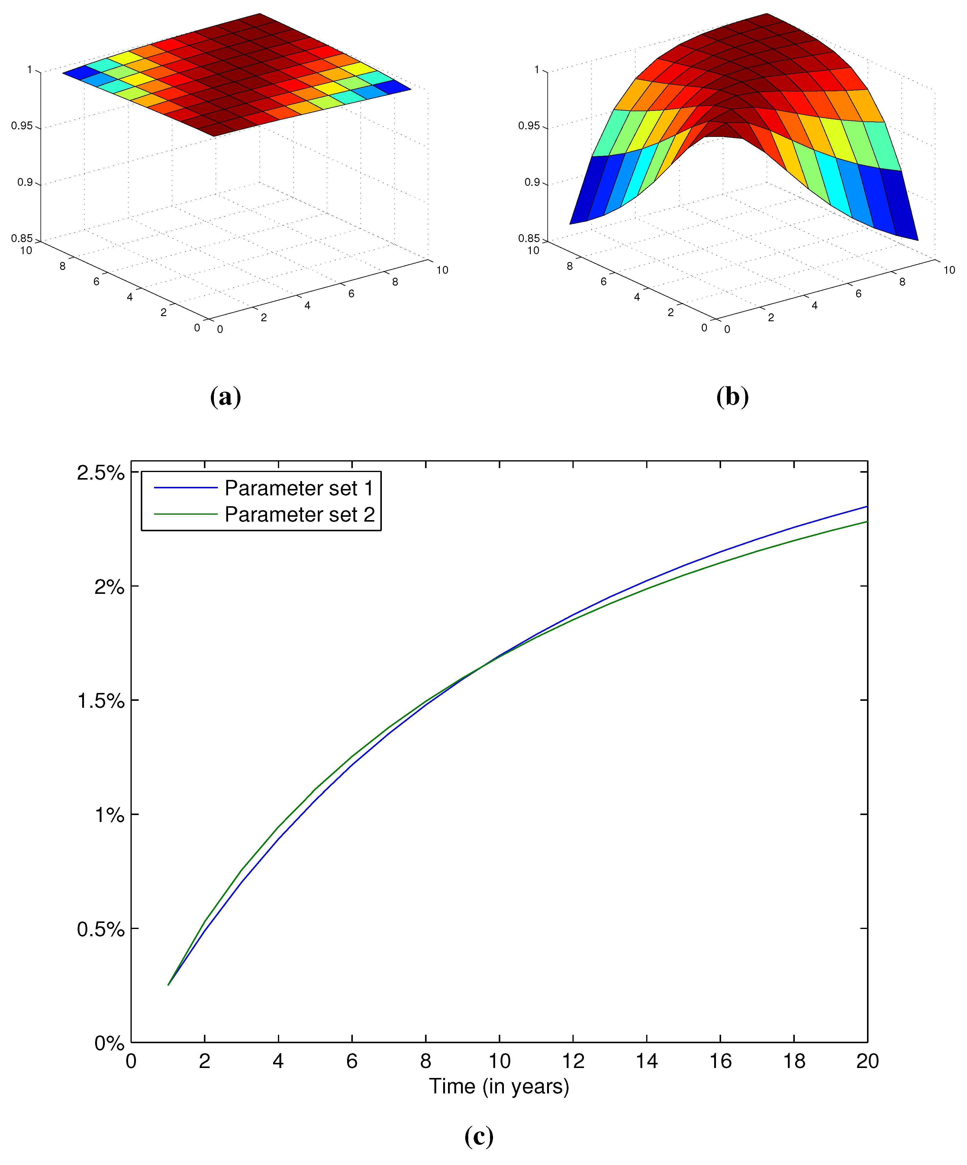
Figure 1. Correlations and yield curves for Parameter sets 1 and 2. (a) Correlation between bond prices for Parameter set 1; (b) Correlation between bond prices Parameter set 2; (c) Yield curves obtained using no-arbitrage bond prices.

Figure 1. Correlations and yield curves for Parameter sets 1 and 2. (a) Correlation between bond prices for Parameter set 1; (b) Correlation between bond prices Parameter set 2; (c) Yield curves obtained using no-arbitrage bond prices.

4.1.1. Numerical Illustration 1: Parameter Sets

We first consider two parameter sets leading to very different covariance structures for zero-coupon bond prices. The two parameter sets are described in Table 1. The main difference between the two parameter sets lies in the second factor. In the first set, a lower $k_2$ causes the effect of the second factor to last as maturities increase. In addition, $g_2$ is higher in the second parameter set, which increases the volatility of the spot rate. The resulting correlation structure between bond prices of times to maturity from ranging from 2 to 10 years are presented in Figure 1.

4.1.2. Numerical Illustration 1: Projected Yield Curve

Using the two parameter sets and Theorem 1, we compare the yield curve derived from best-estimate zero-coupon bond prices to the no-arbitrage one. Note that we can calculate the no-arbitrage price of any zero-coupon bond once a state-price deflator is given. The no-arbitrage price thus obtained is defined with respect to this state-price deflator. However, in practical situations this price is not helpful because incompleteness implies that this instrument is not necessarily traded. Therefore, in an insurance context, this price is not a market price, but a marked-to-model price obtained by market-consistent valuation.

More specifically, we calculate the yield curve from no-arbitrage bond prices obtained from (3), while the best-estimate yield curve is at time t obtained by

$$\ell >0\mapsto R(t,t+\ell )=-\frac{1}{\ell }log\left({\pi }_t\left({\xi }_{t+\ell }\right)\right),$$

(8)

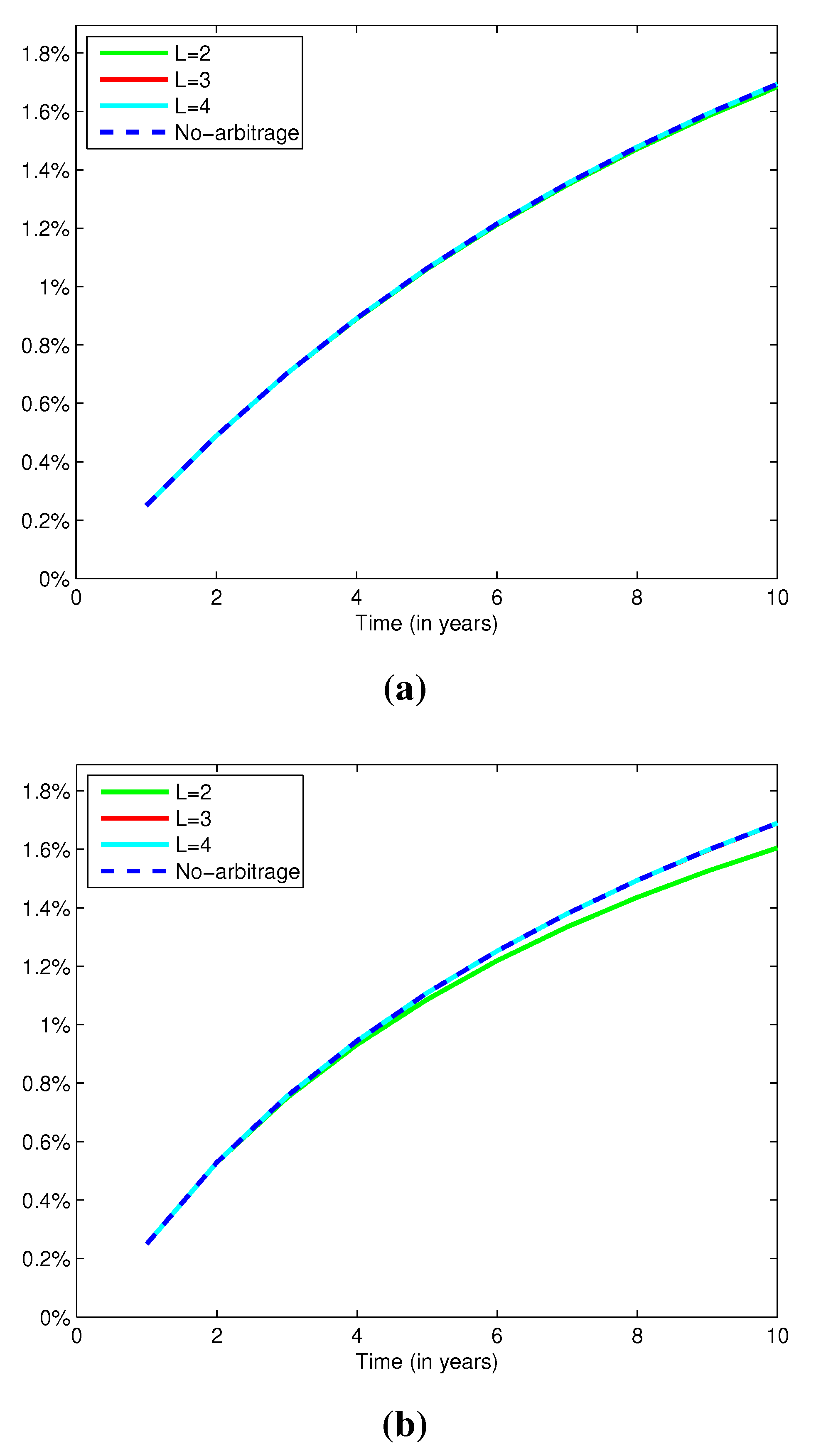
with ${\xi }_{t+\ell }=1$ at time $t+\ell$. The resulting yield curves for bond markets containing $L=$ 2, 3 and 4 bonds are presented in Figure 2. The yield curves are almost visually indistinguishable, so the differences between the best-estimate and the no-arbitrage yields are presented in Table 2.

The absolute differences between best-estimate and no-arbitrage spot yields increase with time to maturity. This phenomenon is accentuated when bond correlation decreases faster as time to maturity increases. As expected, when short- and long-term bonds present a lower correlation, the former are not as useful for replicating the latter. The results in Table 2 also show that the best-estimate yield curves approach the no-arbitrage one when the number (and the maturity) of traded bonds increase.

It is also important to note that the sign of the differences presented in Table 2 is negative in all cases, except for the second parameter set when $L=4$. A negative difference means that the best-estimate bond price is less than the no-arbitrage one, while the opposite is true when the difference is positive. One might assume that the best-estimate yield should always be higher than the no-arbitrage one, to account for reinvestment risk. However, the replicating strategy underlying the best-estimate price allows for short positions, which can result in potential profits, thus reducing the best-estimate price. Furthermore, the best-estimate bond price is defined by a quadratic hedging criteria, which treats deviations above and below the target in a similar way. Thus, best-estimate prices above and below the no-arbitrage price can be expected. Finally, the deviations from the no-arbitrage yield for both parameter sets are very small, and they decrease as L increases.

Figure 2. No-arbitrage and best-estimate projected yield curves. (a) Parameter set 1; (b) Parameter set 2.

Figure 2. No-arbitrage and best-estimate projected yield curves. (a) Parameter set 1; (b) Parameter set 2.

Table 2. Differences between the best-estimate and the no-arbitrage yields for different numbers L of traded bonds, for Parameter sets 1 and 2. Entries 0.0000 and -0.0000 indicate positive and negative numbers whose absolute value is less than ${10}^{-8}$.

Difference between Best-Estimate and No-Arbitrage Yields $(\times {\mathbf{10}}^{-\mathbf{4}})$
Time to
Maturity	3	4	5	6	7	8	9	10
Parameter set 1
$L=2$	$-0.0497$	$-0.1355$	$-0.2475$	$-0.3779$	$-0.5211$	$-0.6727$	$-0.8294$	$-0.9887$
$L=3$	0	$-0.0004$	$-0.0016$	$-0.0037$	$-0.0069$	$-0.0112$	$-0.0167$	$-0.0234$
$L=4$	0	0	$-0.0000$	$-0.0000$	$-0.0000$	$-0.0001$	$-0.0003$	$-0.0005$
Parameter set 2
$L=2$	$-0.4996$	$-1.2757$	$-2.2378$	$-3.3359$	$-4.5347$	$-5.8052$	$-7.1227$	$-8.4663$
$L=3$	0	$-0.0001$	$-0.0023$	$-0.0064$	$-0.0115$	$-0.0170$	$-0.0220$	$-0.0263$
$L=4$	0	0	$0.0000$	$0.0005$	$0.0017$	$0.0037$	$0.0066$	$0.0105$

Table 2. Differences between the best-estimate and the no-arbitrage yields for different numbers L of traded bonds, for Parameter sets 1 and 2. Entries 0.0000 and -0.0000 indicate positive and negative numbers whose absolute value is less than ${10}^{-8}$.

Difference between Best-Estimate and No-Arbitrage Yields $(\times {\mathbf{10}}^{-\mathbf{4}})$
Time to
Maturity	3	4	5	6	7	8	9	10
Parameter set 1
$L=2$	$-0.0497$	$-0.1355$	$-0.2475$	$-0.3779$	$-0.5211$	$-0.6727$	$-0.8294$	$-0.9887$
$L=3$	0	$-0.0004$	$-0.0016$	$-0.0037$	$-0.0069$	$-0.0112$	$-0.0167$	$-0.0234$
$L=4$	0	0	$-0.0000$	$-0.0000$	$-0.0000$	$-0.0001$	$-0.0003$	$-0.0005$
Parameter set 2
$L=2$	$-0.4996$	$-1.2757$	$-2.2378$	$-3.3359$	$-4.5347$	$-5.8052$	$-7.1227$	$-8.4663$
$L=3$	0	$-0.0001$	$-0.0023$	$-0.0064$	$-0.0115$	$-0.0170$	$-0.0220$	$-0.0263$
$L=4$	0	0	$0.0000$	$0.0005$	$0.0017$	$0.0037$	$0.0066$	$0.0105$

4.1.3. Numerical Illustration 1: Sensitivity of the Best-Estimate Yield Curve to λ

In the Vasiček model, each element of the vector λ is proportional to the market risk premium for the associated factor. In this section, we study the impact of increasing the risk premium associated with the first factor. We consider that there are $L=3$ traded bonds in a market governed by Parameter set 1 with different values of λ to assess its influence on the spread between the best-estimate and the no-arbitrage yield curve. 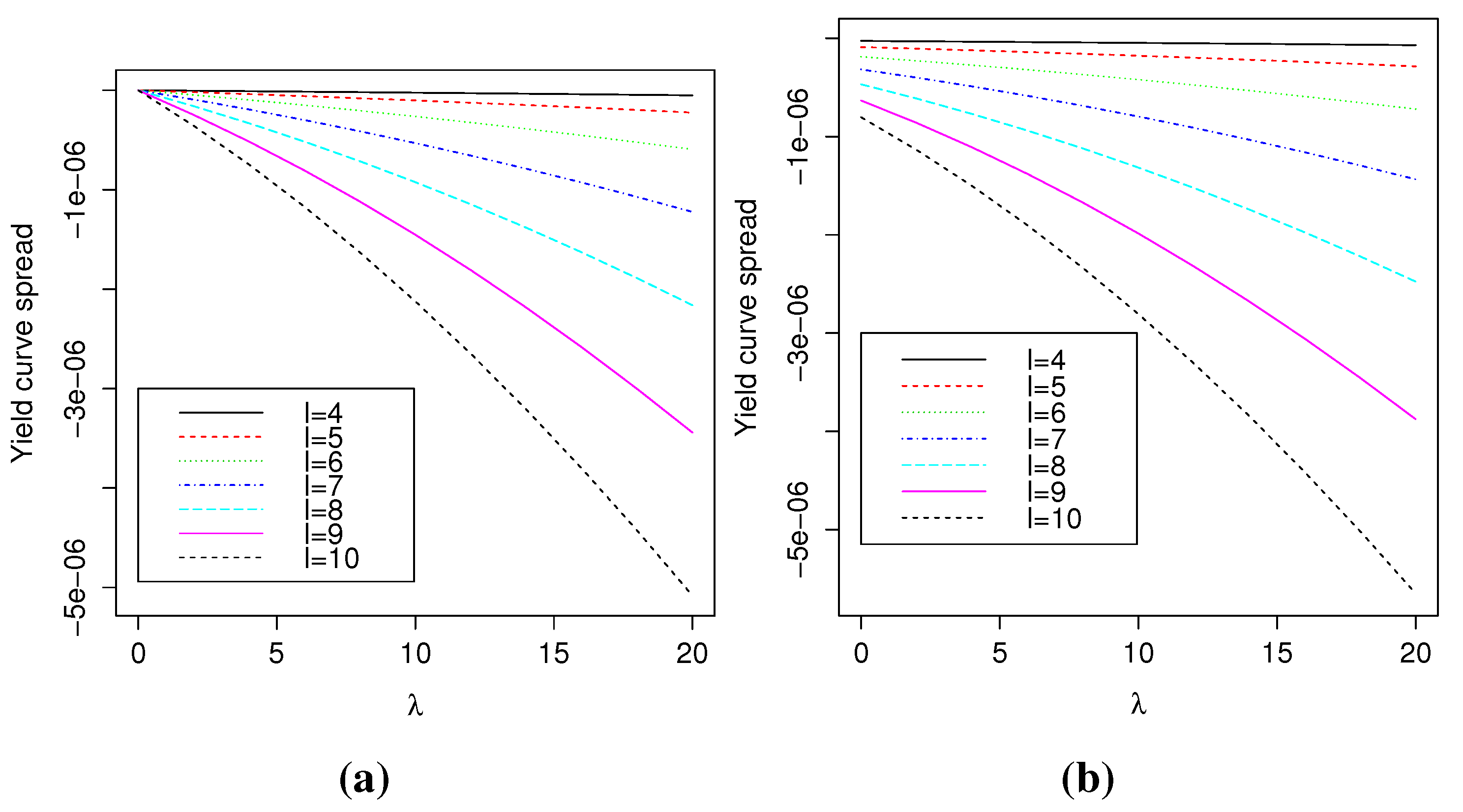The results are presented in Figure 3.

Figure 3. Difference between the best-estimate and no-arbitrage yield for times to maturity ℓ from 4 to 10, $L=3$, for different market risk premium parameter λ. (a) ${\lambda }_2=0$; (b) ${\lambda }_2=15$.

Figure 3. Difference between the best-estimate and no-arbitrage yield for times to maturity ℓ from 4 to 10, $L=3$, for different market risk premium parameter λ. (a) ${\lambda }_2=0$; (b) ${\lambda }_2=15$.

Figure Figure 3 illustrates that the magnitude of the spread increases with ${\lambda }_1$, both for ${\lambda }_2=0$ and ${\lambda }_2=15$. The increase is more important for longer times to maturity. In fact, the market price of risk increases the price of the (risky) hedging strategy underlying the best-estimate yield. Claims with longer times to maturity are riskier to hedge (for a constant number of traded bonds), partly because the strategy must be applied for a longer period, during which errors can accumulate. Observe also that when both risk premium parameters are equal to zero, the best-estimate and no-arbitrage yields coincide. This is not the case when only ${\lambda }_1=0$, because of the positive risk premium for the second factor.

4.1.4. Numerical Illustration 1: Sensitivity to the Number of Factors

It is well-known that at least two factors are necessary to adequately model the term structure of interest rates (see, for example, Section 4.1 of [14]). To test the robustness of our results to a change in the number of factors, we now consider the multifactor Vasiček model with $N=4$. The parameters were chosen such that their resulting yield curves are close to the ones obtained with the two-factor model. Table 3 describes the parameter sets used for this sensitivity test. The resulting risk-neutral yield curve and correlation structure between risk-neutral bond prices are shown in Figure 4.

It is worth noting that in this case, when there are $L=2$ and $L=3$ traded bonds, there are more risk factors in the model than there are traded bonds on the market. This adds to the incompleteness of the market.

Table 3. Parameter sets used for sensitivity to the number of factors, $N=4$.

Parameters	Parameter set 3	Parameter set 4
k	$[0.1360,0.1750,0.0500,0.4000]$	$[0.1360,0.5500,0.2500,0.4500]$
b	$[0.0055,0.0005,0.0005,0.0005]$	$[0.00375,0.0005,0.0005,0.0010]$
g	$[0.0070,0.0042,0.0050,0.0015]$	$[0.0070,0.0075,0.0050,0.0045]$
λ	$[8,15,5,5]$	$[8,15,5,5]$
$y_0$	$[0.003,-0.00025,0.00025,0.00025]$	$[0.003,-0.00025,0.00025,0.00025]$

Table 3. Parameter sets used for sensitivity to the number of factors, $N=4$.

Parameters	Parameter set 3	Parameter set 4
k	$[0.1360,0.1750,0.0500,0.4000]$	$[0.1360,0.5500,0.2500,0.4500]$
b	$[0.0055,0.0005,0.0005,0.0005]$	$[0.00375,0.0005,0.0005,0.0010]$
g	$[0.0070,0.0042,0.0050,0.0015]$	$[0.0070,0.0075,0.0050,0.0045]$
λ	$[8,15,5,5]$	$[8,15,5,5]$
$y_0$	$[0.003,-0.00025,0.00025,0.00025]$	$[0.003,-0.00025,0.00025,0.00025]$

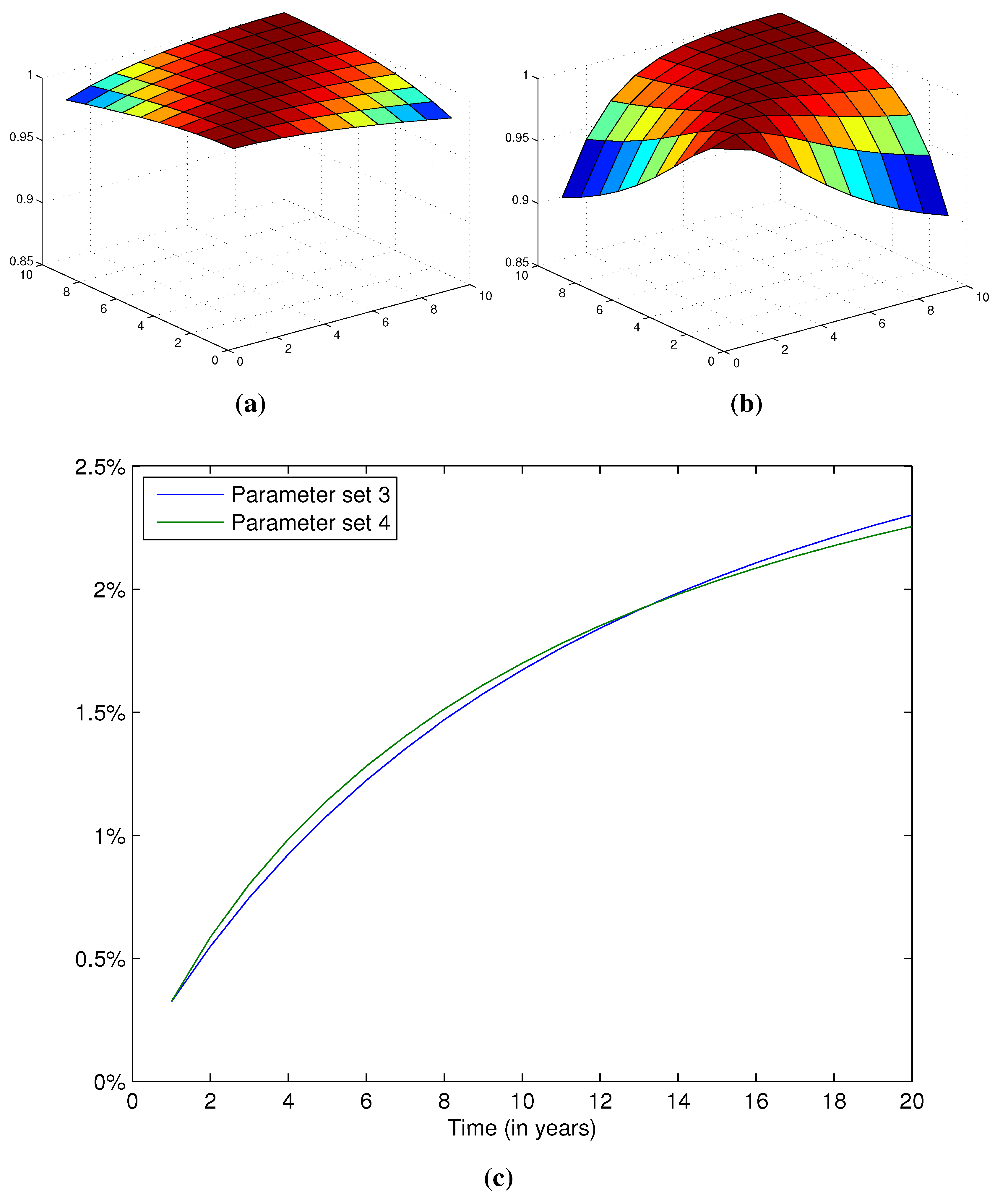
Figure 4. Correlations and yield curves for Parameter sets 3 and 4. (a) Correlation between bond prices for Parameter set 3; (b) Correlation between bond prices for Parameter set 4; (c) Yield curves obtained using no-arbitrage bond prices.

Figure 4. Correlations and yield curves for Parameter sets 3 and 4. (a) Correlation between bond prices for Parameter set 3; (b) Correlation between bond prices for Parameter set 4; (c) Yield curves obtained using no-arbitrage bond prices.

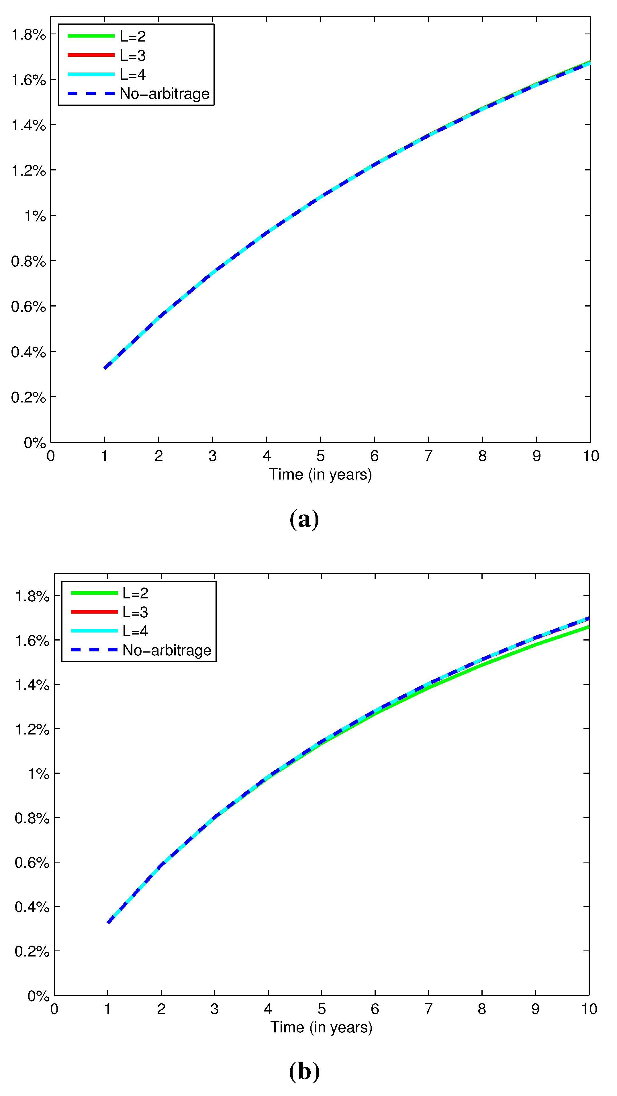
The resulting best-estimate yield curves are illustrated in Figure 5, and the differences between the best-estimate and the no-arbitrage curves are presented in Table 4. The trends obtained under the two-factor model can also be observed with four factors. The most noticeable difference between the no-arbitrage and the best-estimate yield curves happens for longer times to maturity when the market only contains two traded bonds. In that case, the bond market does not contain enough bonds to adequately replicate bonds with longer times to maturity. This is especially true for the second parameter set, since it presents lower correlation between short- and long-term bonds.

Figure 5. No-arbitrage and best-estimate projected yield curves. (a) Parameter set 3; (b) Parameter set 4.

Figure 5. No-arbitrage and best-estimate projected yield curves. (a) Parameter set 3; (b) Parameter set 4.

Notice that for Parameter set 4, the difference between both yield curves is negative, indicating a negative reinvestment risk premium. However, the risk premia remain comparably small and get closer to zero as the number of traded bonds increase.

Table 4. Differences between the best-estimate and the no-arbitrage yields for different numbers L of traded bonds, for Parameter sets 3 and 4.

Difference between Best-Estimate and No-Arbitrage Yields $(\times {\mathbf{10}}^{-\mathbf{4}})$
time to
maturity	3	4	5	6	7	8	9	10
Parameter set 3
$L=2$	$0.0028$	$\phantom{-}0.0174$	$\phantom{-}0.0499$	$\phantom{-}0.1040$	$\phantom{-}0.1822$	$\phantom{-}0.2855$	$\phantom{-}0.4141$	$\phantom{-}0.5679$
$L=3$	0	$\phantom{-}0.0014$	$\phantom{-}0.0063$	$\phantom{-}0.0174$	$\phantom{-}0.0367$	$\phantom{-}0.0664$	$\phantom{-}0.1078$	$\phantom{-}0.1615$
$L=4$	0	$\phantom{-}0$	$\phantom{-}0.0001$	$\phantom{-}0.0006$	$\phantom{-}0.0016$	$\phantom{-}0.0034$	$\phantom{-}0.0063$	$\phantom{-}0.0100$
Parameter set 4
$L=2$	$-0.1397$	$-0.4049$	$-0.7877$	$-1.2766$	$-1.8562$	$-2.5098$	$-3.2208$	$-3.9738$
$L=3$	0	$-0.0033$	$-0.0146$	$-0.0372$	$-0.0729$	$-0.1222$	$-0.1845$	$-0.2589$
$L=4$	0	0	$-0.0003$	$-0.0010$	$-0.0026$	$-0.0053$	$-0.0094$	$-0.0149$

Table 4. Differences between the best-estimate and the no-arbitrage yields for different numbers L of traded bonds, for Parameter sets 3 and 4.

Difference between Best-Estimate and No-Arbitrage Yields $(\times {\mathbf{10}}^{-\mathbf{4}})$
time to
maturity	3	4	5	6	7	8	9	10
Parameter set 3
$L=2$	$0.0028$	$\phantom{-}0.0174$	$\phantom{-}0.0499$	$\phantom{-}0.1040$	$\phantom{-}0.1822$	$\phantom{-}0.2855$	$\phantom{-}0.4141$	$\phantom{-}0.5679$
$L=3$	0	$\phantom{-}0.0014$	$\phantom{-}0.0063$	$\phantom{-}0.0174$	$\phantom{-}0.0367$	$\phantom{-}0.0664$	$\phantom{-}0.1078$	$\phantom{-}0.1615$
$L=4$	0	$\phantom{-}0$	$\phantom{-}0.0001$	$\phantom{-}0.0006$	$\phantom{-}0.0016$	$\phantom{-}0.0034$	$\phantom{-}0.0063$	$\phantom{-}0.0100$
Parameter set 4
$L=2$	$-0.1397$	$-0.4049$	$-0.7877$	$-1.2766$	$-1.8562$	$-2.5098$	$-3.2208$	$-3.9738$
$L=3$	0	$-0.0033$	$-0.0146$	$-0.0372$	$-0.0729$	$-0.1222$	$-0.1845$	$-0.2589$
$L=4$	0	0	$-0.0003$	$-0.0010$	$-0.0026$	$-0.0053$	$-0.0094$	$-0.0149$

4.2. Numerical Illustration 2: Life Insurance Inspired

This second example is inspired by the long-term liabilities that insurers need to value, and the bonds that may be available to them. So far, we have limited ourselves to bonds with maturities of 4 years or less. However, many markets are deep and liquid for bonds with times to maturity up to 10 years or more. Thus, in this example, we consider a claim with 11 to 20 years to maturity, which we price and hedge using bonds with times to maturity up to 10 years.

The prices of bonds with times to maturity close to each other tend to be highly correlated. For this reason, selected bonds with times to maturity further apart can be sufficient to replicate long-term bonds in a satisfactory manner. From a numerical and computational point of view, this is also an advantage. Indeed, when $L=10$, the resulting covariance matrix is often ill-conditioned, making calculations impractical and imprecise. This is due to the quasi-linear dependence between the prices of bonds with similar times to maturity. Replicating long-term claims using less (but well-chosen) bonds also reduces the magnitude of the long and short positions that must be taken to cover the liability.

In this numerical example, we assume that for each trading period, the hedge is built using bonds with times to maturity $m\in ℳ=\{m_1,...,m_L\}$, with $L\le 10$. Here we choose the following examples: $ℳ=\{1,10\}$, $ℳ=\{1,2,10\}$, $ℳ=\{1,5,10\}$, $ℳ=\{1,2,5,10\}$. In fact, yield curves can often be interpolated using only a few bonds with well-chosen times to maturity (see, for example, Section 3.6 of [15]). Note that if we assume that there are gaps in the times to maturity tensors $ℳ$ then we slightly need to change the formulas presented in Theorem 1 and Proposition 1. For simplicity reasons we avoid further details.

4.2.1. Numerical Illustration 2: Parameter Set

We consider a three-factor Vasiček model with parameters that match the actual yield curve interpolated from the prices of Swiss Confederation bonds on 1 March 2005. Three factors are generally sufficient to capture the evolution of the market yield curve (see Section 3.6 of [15,16]). We choose the parameters described in Table 5. The resulting yield curve and bond price correlations are presented in Figure 6.

Table 5. Parameter set used for Example 3 for N = 3.

Parameters	Parameter set 5
k	$[0.1600,0.5214,0.2728]$
b	$[0.0060,0.0005,0.0005]$
g	$[0.0060,0.0064,0.0042]$
λ	$[7.8704,13.8290,4.6956]$
$y_0$	$[0.0079,0.0005,0.0005]$

Table 5. Parameter set used for Example 3 for N = 3.

Parameters	Parameter set 5
k	$[0.1600,0.5214,0.2728]$
b	$[0.0060,0.0005,0.0005]$
g	$[0.0060,0.0064,0.0042]$
λ	$[7.8704,13.8290,4.6956]$
$y_0$	$[0.0079,0.0005,0.0005]$

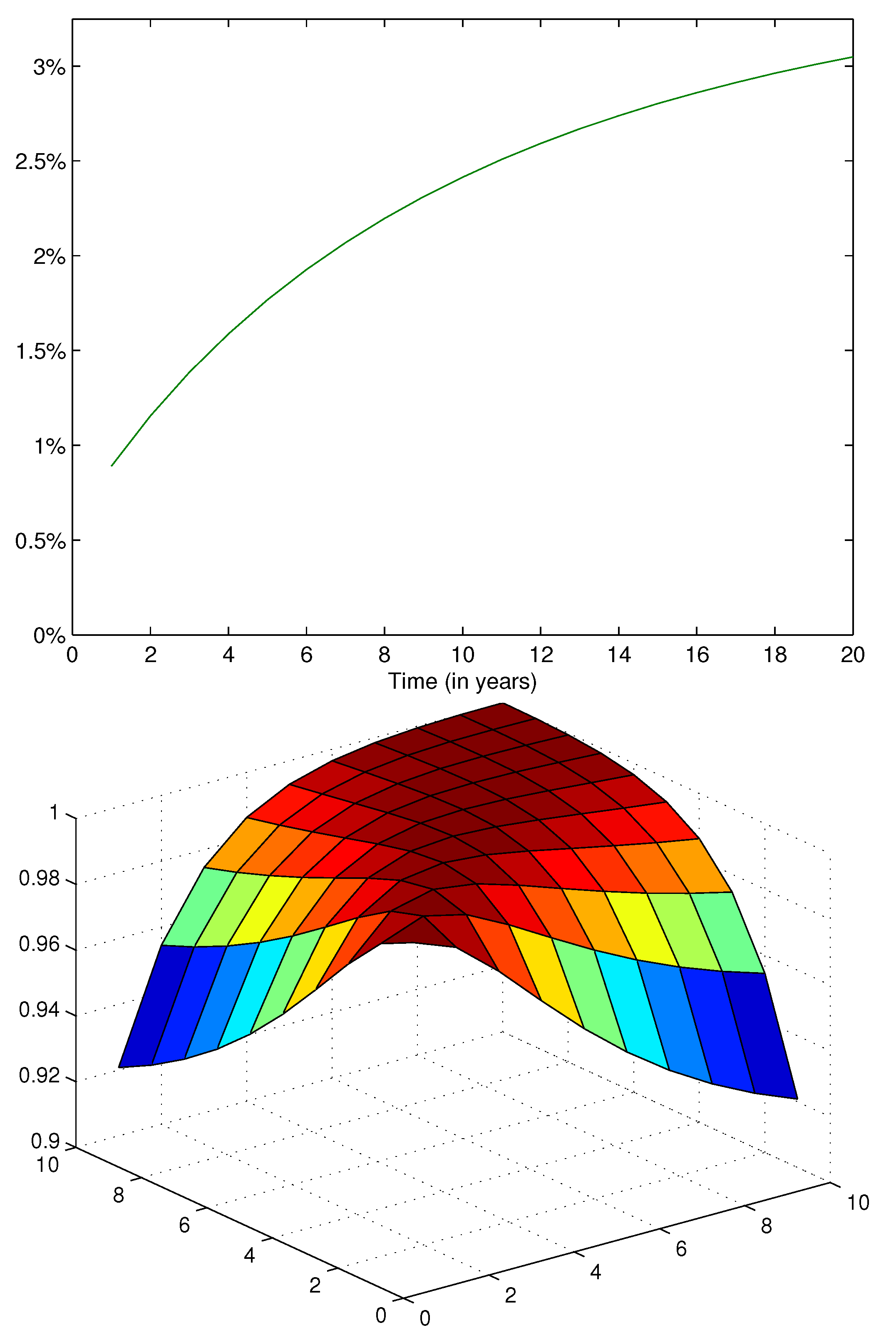
Figure 6. Correlation and yield curve for Parameter set 5.

Figure 6. Correlation and yield curve for Parameter set 5.

4.2.2. Numerical Illustration 2: Projected Yield Curve

Again, we calculate the best-estimate yield curve resulting from the best-estimate prices of bonds. This time we focus on maturities ranging from 11 to 20 years. The differences between the best-estimate yield curve and the no-arbitrage one are presented in Table 6. As in the previous example, the absolute difference between both yield curves increases with time to maturity. A larger number of bonds used in the hedging portfolio also helps to reduce the difference between the best-estimate and the no-arbitrage yield curve. The second and third lines of Table 6 show that the choice of the bonds to include in the portfolio has an impact on the difference. In fact, when $ℳ=\{1,5,10\}$, the no-arbitrage yield curve is better replicated compared to $ℳ=\{1,2,10\}$, which makes sense since the bond with 5 years to maturity is better able to complete the other bonds in capturing the no-arbitrage yield curve.

Table 6. Differences between the best-estimate and the no-arbitrage yields for different sets of traded bonds, for Parameter set 5.

Difference between Best-Estimate and No-Arbitrage Yields $(\times {\mathbf{10}}^{-\mathbf{6}})$
Time to
Maturity	11	12	13	14	15	16	17	18	19	20
$ℳ=\{1,10\}$	$-1.2626$	$-3.9880$	$-8.1578$	$-13.6365$	$-20.2351$	$-27.7488$	$-35.9780$	$-44.7389$	$-53.8692$	$-63.2290$
$ℳ=\{1,2,10\}$	$-0.3343$	$-1.0648$	$-2.1920$	$-3.6848$	$-5.4973$	$-7.5781$	$-9.8757$	$-12.341$	$-14.9308$	$-17.6051$
$ℳ=\{1,5,10\}$	$-0.1594$	$-0.5152$	$-1.07332$	$-1.8229$	$-2.7437$	$-3.8115$	$-5.0009$	$-6.2870$	$-7.6467$	$-9.0592$
$ℳ=\{1,2,5,10\}$	$-0.0007$	$-0.0009$	$-0.0009$	$-0.0012$	$-0.0023$	$-0.0046$	$-0.0081$	$-0.0130$	$-0.0194$	$-0.0273$

Table 6. Differences between the best-estimate and the no-arbitrage yields for different sets of traded bonds, for Parameter set 5.

Difference between Best-Estimate and No-Arbitrage Yields $(\times {\mathbf{10}}^{-\mathbf{6}})$
Time to
Maturity	11	12	13	14	15	16	17	18	19	20
$ℳ=\{1,10\}$	$-1.2626$	$-3.9880$	$-8.1578$	$-13.6365$	$-20.2351$	$-27.7488$	$-35.9780$	$-44.7389$	$-53.8692$	$-63.2290$
$ℳ=\{1,2,10\}$	$-0.3343$	$-1.0648$	$-2.1920$	$-3.6848$	$-5.4973$	$-7.5781$	$-9.8757$	$-12.341$	$-14.9308$	$-17.6051$
$ℳ=\{1,5,10\}$	$-0.1594$	$-0.5152$	$-1.07332$	$-1.8229$	$-2.7437$	$-3.8115$	$-5.0009$	$-6.2870$	$-7.6467$	$-9.0592$
$ℳ=\{1,2,5,10\}$	$-0.0007$	$-0.0009$	$-0.0009$	$-0.0012$	$-0.0023$	$-0.0046$	$-0.0081$	$-0.0130$	$-0.0194$	$-0.0273$

5. Conclusions

We apply the definition of best-estimate given by [6] in terms of span-deflators to price long-term bonds in a market with reinvestment risk. We assume that there exists a limited number of traded bonds, whose linear combination form a space of one-period replicable payoffs. We value the long-term claim recursively and obtain the best-estimate price using a series of orthogonal projections on the space of replicable payoffs. This allows to distinguish between the hedgeable and non-hedgeable parts of the claim. We then consider a multifactor Vasiček model and obtain analytical expressions for the aggregate market span-deflator, the best-estimate price of long-term bonds and the hedging portfolio. Through numerical examples, we show that as the number of bonds included in the portfolio increases, the best-estimate yield curve approaches the no-arbitrage one. For longer maturities, it is harder to replicate the no-arbitrage yield curve using a limited number of bonds. By carefully picking the bonds to include in the hedging portfolio, it is possible to obtain a yield curve that is close to the no-arbitrage one without increasing the number of bonds in the portfolio.

The main goal of this paper was to obtain the best-estimate price of long-term bonds when only a limited number of shorter term bonds can be traded. Orthogonal projections on a space of replicable payoffs allowing short positions extend the conditional expectation in a natural way. The resulting best-estimate yield curve is very close to the no-arbitrage one prescribed by the model, and no significant reinvestment risk premium can be observed. However, the hedging strategy underlying the best-estimate price is not necessarily realistic for insurers, since they typically do not take short positions in bonds. The best-estimate yield curve also does not take model risk into account.

6. Proofs

Proof of Lemma 3.

  We use the first two moments of the bond price in the discrete time multifactor Vasiček model from Section 3.6 of [15] to derive an expression for the market span-deflator. We have

$$\begin{array}{ccc}\hfill p_{t,s}=𝔼\left.\left[P(t,t+s)\right|{ℱ}_{t-1}\right]& =& \text{exp}\left\{A\left(s\right)-\sum _{j=1}^N{B}_j\left(s\right)\left[b_j+{\beta }_j{Y}_j(t-1)\right]+\frac{1}{2}\sum _{j=1}^N{g}_j^2{B}_j{\left(s\right)}^2\right\}\hfill \end{array}$$

and

$$\begin{array}{ccc}\hfill \mathrm{Cov}\left.\left(P(t,t+s),P(t,t+u)\right|{ℱ}_{t-1}\right)& =& p_{t,s}{p}_{t,u}\left(\text{exp}\left\{\sum _{j=1}^N{g}_j^2{B}_j\left(s\right)B_j\left(u\right)\right\}-1\right)\hfill \end{array}$$

Using the notation defined in Section 3, this implies

$$\begin{array}{ccc}\hfill {\text{Σ}}_{t-1}& =& \mathrm{diag}{\left(p_{t,s}\right)}_{s=1,...,L-1}{\left(\text{exp}\left\{\sum _{j=1}^N{g}_j^2{B}_j\left(s\right)B_j\left(u\right)\right\}-1\right)}_{s,u=1,...,L-1}\mathrm{diag}{\left(p_{t,s}\right)}_{s=1,...,L-1}\hfill \\ & =& \mathrm{diag}\left({\tilde{{p}}}_t\right)C\mathrm{diag}\left({\tilde{{p}}}_t\right)\hfill \end{array}$$

Moreover, by the definition of ${\breve{\phi }}_t$, we have

$$𝔼\left[\left.{\breve{\phi }}_t\right|{ℱ}_{t-1}\right]=\text{exp}\{-r_{t-1}\}=\text{exp}\left\{-\sum _{j=1}^N{Y}_j(t-1)\right\}$$

and

$$\begin{array}{ccc}\hfill {{v}}_{t-1}\left({\breve{\phi }}_t\right)& =& {\left(p_{t,s}\text{exp}\left\{-\sum _{j=1}^N{Y}_j(t-1)\right\}\left(\text{exp}\left\{-\sum _{j=1}^N{\lambda }_j{g}_j{B}_j\left(s\right)Y_j(t-1)\right\}-1\right)\right)}_{s=1,...,L-1}\hfill \\ & =& \text{exp}\{-r_{t-1}\}\mathrm{diag}\left({\tilde{{p}}}_t\right){\left(\text{exp}\left\{-\sum _{j=1}^N{\lambda }_j{g}_j{B}_j\left(s\right)Y_j(t-1)\right\}-1\right)}_{s=1,...,L-1}\hfill \\ & =& \text{exp}\{-r_{t-1}\}\mathrm{diag}\left({\tilde{{p}}}_t\right){w}\left({Y}(t-1)\right)\hfill \end{array}$$

Setting ${\tilde{{1}}}^{\prime }=(1,...,1)={\tilde{{p}}}_t^{\prime }\mathrm{diag}{\left({\tilde{{p}}}_t\right)}^{-1}$, this implies

$$\begin{array}{ccc}\hfill {\breve{\psi }}_t& =& {\mathrm{Q}}_H^t{\breve{\phi }}_t=e^{-r_{t-1}}-{\tilde{{p}}}_t^{\prime }{\text{Σ}}_{t-1}^{-1}{{v}}_{t-1}\left({\breve{\phi }}_t\right)+{\tilde{{P}}}_t^{\prime }{\text{Σ}}_{t-1}^{-1}{{v}}_{t-1}\left({\breve{\phi }}_t\right)\hfill \\ & =& e^{-r_{t-1}}-e^{-r_{t-1}}{\tilde{{1}}}^{\prime }{C}^{-1}{w}\left({Y}(t-1)\right)+e^{-r_{t-1}}{\tilde{{P}}}_t^{\prime }\mathrm{diag}{\left({\tilde{{p}}}_t\right)}^{-1}{C}^{-1}{w}\left({Y}(t-1)\right)\hfill \end{array}$$

Observe that

$${\tilde{{P}}}_t^{\prime }\mathrm{diag}{\left({\tilde{{p}}}_t\right)}^{-1}{C}^{-1}={\left(\text{exp}\left\{-\sum _{j=1}^N{g}_j^2{B}_j{\left(s\right)}^2/2+g_j{B}_j\left(s\right){\epsilon }_{j,t}\right\}\right)}_{s=1,...,L-1}^{\prime }{C}^{-1}={z}{\left({\epsilon }_t\right)}^{\prime }$$

Under these assumptions, and recalling that ${{c}}^{\prime }={\tilde{{1}}}^{\prime }{C}^{-1}$, we obtain the desired result. □

Proof of Theorem 1.

  First, we show that the claim holds for $\ell =L+1$, which initializes the recursion. We have by the tower property of conditional expectation and using Lemma 3

$$\begin{array}{cc}\hfill 𝔼\left.\left[\prod _{u=t+1}^{t+L+1}{\breve{\psi }}_u\right|{ℱ}_t\right]& =𝔼\left.\left[{\breve{\psi }}_{t+1}𝔼\left.\left[\prod _{u=t+2}^{t+L+1}{\breve{\psi }}_u\right|{ℱ}_{t+1}\right]\right|{ℱ}_t\right]=𝔼\left.\left[{\breve{\psi }}_{t+1}P(t+1,t+L+1)\right|{ℱ}_t\right]\hfill \\ & =𝔼\left.\left[e^{-{\sum }_{j=1}^N{Y}_j\left(t\right)}\left(1-{{c}}^{\prime }{w}\left({Y}\left(t\right)\right)+{z}{\left({\epsilon }_{t+1}\right)}^{\prime }{w}\left({Y}\left(t\right)\right)\right)P(t+1,t+L+1)\right|{ℱ}_t\right]\hfill \\ & =e^{-{\sum }_{j=1}^N{Y}_j\left(t\right)}\left\{\left(1-{{c}}^{\prime }{w}\left({Y}\left(t\right)\right)\right)𝔼\left.\left[P(t+1,t+L+1)\right|{ℱ}_t\right]\right.\hfill \\ & +\left.𝔼\left.\left[{z}{\left({\epsilon }_{t+1}\right)}^{\prime }{w}\left({Y}\left(t\right)\right)P(t+1,t+L+1)\right|{ℱ}_t\right]\right\}\hfill \end{array}$$

We calculate these expected values on the right-hand side.

$$\begin{array}{cc}& e^{-{\sum }_{j=1}^N{Y}_j\left(t\right)}\left(1-{{c}}^{\prime }{w}\left({Y}\left(t\right)\right)\right)𝔼\left.\left[P(t+1,t+L+1)\right|{ℱ}_t\right]\hfill \\ & =e^{-{\sum }_{j=1}^N{Y}_j\left(t\right)}\left(1-{{c}}^{\prime }{w}\left({Y}\left(t\right)\right)\right)e^{A\left(L\right)-{\sum }_{j=1}^N\left\{(b_j+{\beta }_j{Y}_j\left(t\right))B_j\left(L\right)+\frac{g_j^2}{2}{\left(B_j\left(L\right)\right)}^2\right\}}\hfill \\ & =\left(1-{{c}}^{\prime }{w}\left({Y}\left(t\right)\right)\right)e^{A^{\left(0\right)}(L+1)-{\sum }_{j=1}^N{Y}_j\left(t\right)(1+{\beta }_j{B}_j\left(L\right))}\hfill \\ & =\left(1-{{c}}^{\prime }{w}\left({Y}\left(t\right)\right)\right)e^{A^{\left(0\right)}(L+1)-{\sum }_{j=1}^N{Y}_j\left(t\right)B_j^{\left(0\right)}(L+1)}\hfill \\ & =(1+{{c}}^{\prime }\tilde{{1}})e^{A^{\left(0\right)}(L+1)-{\sum }_{j=1}^N{Y}_j\left(t\right)B_j^{\left(0\right)}(L+1)}-{{c}}^{\prime }{\left(e^{A^{\left(s\right)}(L+1)-{\sum }_{j=1}^N{Y}_j\left(t\right)B_j^{\left(s\right)}(L+1)}\right)}_{s=1,...,L-1}^{\prime }\hfill \end{array}$$

Letting $c_{s,u}$ denote the $u^{\text{th}}$ term in the $s^{\text{th}}$ row of C, the second term is

$$\begin{array}{cc}& e^{-{\sum }_{j=1}^N{Y}_j\left(t\right)}𝔼\left.\left[{z}{\left({\epsilon }_{t+1}\right)}^{\prime }{w}\left({Y}\left(t\right)\right)P(t+1,t+L+1)\right|{ℱ}_t\right]\hfill \\ & =e^{-{\sum }_{j=1}^N{Y}_j\left(t\right)}\sum _{s=1}^{L-1}\sum _{u=1}^{L-1}{c}_{s,u}^{-1}(e^{-{\sum }_{j=1}^N{\lambda }_j{g}_{j}B\left(u\right)Y_j\left(t\right)}-1)\hfill \\ & 𝔼\left[\left.e^{-{\sum }_{j=1}^N\left(\frac{g_j^2}{2}{B}_j{\left(s\right)}^2+g_j{B}_j\left(s\right){\epsilon }_{j,t+1}\right)+A\left(L\right)-{\sum }_{j=1}^N{Y}_j(t+1)B\left(L\right)}\right|{ℱ}_t\right]\hfill \\ & =\sum _{s=1}^{L-1}\sum _{u=1}^{L-1}{c}_{s,u}^{-1}{e}^{{\sum }_{j=1}^N{g}_j^2{B}_j\left(s\right)B_j\left(L\right)}\left(e^{A^{\left(u\right)}(L+1)-{\sum }_{j=1}^N{Y}_j\left(t\right)B^{\left(u\right)}(L+1)}-e^{A^{\left(0\right)}(L+1)-{\sum }_{j=1}^N{Y}_j\left(t\right)B^{\left(0\right)}(L+1)}\right)\hfill \\ & ={\left(e^{{\sum }_{j=1}^N{g}_j^2{B}_j\left(s\right)B_j\left(L\right)}\right)}_{s=1,...,L-1}{C}^{-1}{\left(e^{A^{\left(s\right)}(L+1)-{\sum }_{j=1}^N{Y}_j\left(t\right)B_j^{\left(s\right)}(L+1)}\right)}_{s=1,...,L-1}^{\prime }\hfill \\ & -{\left(e^{{\sum }_{j=1}^N{g}_j^2{B}_j\left(s\right)B_j\left(L\right)}\right)}_{s=1,...,L-1}{C}^{-1}\tilde{{1}}{e}^{A^{\left(0\right)}(L+1)-{\sum }_{j=1}^N{Y}_j\left(t\right)B_j^{\left(0\right)}(L+1)}\hfill \end{array}$$

Collecting all terms and using (5) and (6) provides

$$\begin{array}{cc}\hfill 𝔼\left.\left[\prod _{u=t+1}^{t+L+1}{\breve{\psi }}_u\right|{ℱ}_t\right]& =\left(1-{\left(e^{{\sum }_{j=1}^N{g}_j^2{B}_j\left(s\right)B_j\left(L\right)}-1\right)}_{s=1,...,L-1}{C}^{-1}\tilde{{1}}\right)e^{A^{\left(0\right)}(L+1)-{\sum }_{j=1}^N{Y}_j\left(t\right)B^{\left(0\right)}(L+1)}\hfill \\ & +{\left(e^{{\sum }_{j=1}^N{g}_j^2{B}_j\left(s\right)B_j\left(L\right)}-1\right)}_{s=1,...,L-1}{C}^{-1}{\left(e^{A^{\left(s\right)}(L+1)-{\sum }_{j=1}^N{Y}_j\left(t\right)B^{\left(s\right)}(L+1)}\right)}_{s=1,...,L-1}\hfill \\ & =M_0(L+1)e^{A^{\left(0\right)}(L+1)-{\sum }_{j=1}^N{Y}_j\left(t\right)B_j^{\left(0\right)}(L+1)}\hfill \\ & +{\varsigma }_1(L+1)e^{A^{\left(1\right)}(L+1)-{\sum }_{j=1}^N{Y}_j\left(t\right)B_j^{\left(1\right)}(L+1)}\hfill \\ & +...+{\varsigma }_{L-1}(L+1)e^{A^{(L-1)}(L+1)-{\sum }_{j=1}^N{Y}_j\left(t\right)B_j^{(L-1)}(L+1)}\hfill \\ & =\sum _{i=0}^{L-1}{\omega }_i(L+1)e^{A^{\left(i\right)}(L+1)-{\sum }_{j=1}^N{Y}_j\left(t\right)B_j^{\left(i\right)}(L+1)}\hfill \end{array}$$

Now, we suppose that the claim holds for all $k\in \{L+1,L+2,...,\ell \}$, and we show that it also holds for $\ell +1$. To do so, it suffices to observe that for any $i\in \{0,...,L^{\ell -L}-1\}$,

$$\begin{array}{cc}& 𝔼\left.\left[{\breve{\psi }}_{t+1}{\omega }_i\left(\ell \right)e^{A^{\left(i\right)}\left(\ell \right)-{\sum }_{j=1}^N{Y}_j(t+1)B_j^{\left(i\right)}\left(\ell \right)}\right|{ℱ}_t\right]\hfill \\ & ={\omega }_i\left(\ell \right)𝔼\left.\left[e^{-{\sum }_{j=1}^N{Y}_j\left(t\right)}\left(1-{{c}}^{\prime }{w}\left({Y}\left(t\right)\right)+{z}{\left({\epsilon }_{t+1}\right)}^{\prime }{w}\left({Y}\left(t\right)\right)\right)e^{A^{\left(i\right)}\left(\ell \right)-{\sum }_{j=1}^N{Y}_j(t+1)B_j^{\left(i\right)}\left(\ell \right)}\right|{ℱ}_t\right]\hfill \\ & ={\omega }_i\left(\ell \right)\{\left(1-{\left(e^{{\sum }_{j=1}^N{g}_j^2{B}_j\left(s\right)B_j^{\left(i\right)}\left(\ell \right)}-1\right)}_{s=1,...,L-1}{C}^{-1}\tilde{{1}}\right)e^{A^{\left(iL\right)}(\ell +1)-{\sum }_{j=1}^N{Y}_j\left(t\right)B^{\left(iL\right)}(\ell +1)}\hfill \\ & +{\left(e^{{\sum }_{j=1}^N{g}_j^2{B}_j\left(s\right)B_j^{\left(i\right)}\left(\ell \right)}-1\right)}_{s=1,...,L-1}{C}^{-1}{\left(e^{A^{(iL+s)}(\ell +1)-{\sum }_{j=1}^N{Y}_j\left(t\right)B^{(iL+s)}(\ell +1)}\right)}_{s=1,...,L-1}\}\hfill \\ & ={\omega }_i\left(\ell \right)\left(M_{iL}(\ell +1)e^{A(\ell +1)-{\sum }_{j=1}^N{Y}_j\left(t\right)B_j^{\left(iL\right)}(\ell +1)}\right)\hfill \\ & +{\varsigma }_{iL+1}(\ell +1)e^{A(\ell +1)-{\sum }_{j=1}^N{Y}_j\left(t\right)B_j^{(iL+1)}(\ell +1)}+...+{\varsigma }_{iL+L-1}(m+1)e^{A(\ell +1)-{\sum }_{j=1}^N{Y}_j\left(t\right)B_j^{(iL+L-1)}(\ell +1)}\hfill \\ & =\sum _{i=0}^{L^{\ell +1}-1}{\omega }_i(\ell +1)e^{A^{\left(i\right)}(\ell +1)-{\sum }_{j=1}^N{Y}_j\left(t\right)B_j^{\left(i\right)}(\ell +1)}\hfill \end{array}$$

Note that the second equality above stems from the fact that this term has the same affine structure as when $\ell =L+1$, only with different constants. To obtain the last equality, we use the definition of ${\omega }_i\left(\ell \right)$.  □

Proof of Proposition 1.

  Observe that, using Theorem 1, we can calculate the best-estimate price at t of a bond with time to maturity $\ell >L$, (i.e., for payoff ${\xi }_{t+\ell }=1$ at time $t+\ell$) as

$$\begin{array}{cc}\hfill {\pi }_t\left({\xi }_{t+\ell }\right)& =𝔼\left.\left[\prod _{u=t+1}^{t+\ell }{\breve{\psi }}_u\right|{ℱ}_t\right]=𝔼\left.\left[{\breve{\psi }}_{t+1}\sum _{i=0}^{L^{\ell -1-L}-1}\left({\omega }_i(\ell -1)e^{A^{\left(i\right)}(\ell -1)-{\sum }_{j=1}^N{Y}_j(t+1)B_j^{\left(i\right)}(\ell -1)}\right)\right|{ℱ}_t\right]\hfill \\ & =\sum _{i=0}^{L^{\ell -1-L}-1}{\omega }_i(\ell -1)𝔼\left.\left[{\breve{\psi }}_{t+1}\left(e^{A^{\left(i\right)}(\ell -1)-{\sum }_{j=1}^N{Y}_j(t+1)B_j^{\left(i\right)}(\ell -1)}\right)\right|{ℱ}_t\right]\hfill \end{array}$$

Define ${\xi }_{t+1}^i=e^{A^{\left(i\right)}(\ell -1)-{\sum }_{j=1}^N{Y}_j(t+1)B_j^{\left(i\right)}(\ell -1)}$. Then, using (4) to express each expectation in terms of its hedgeable best approximation, we have

$$\begin{array}{cc}\hfill 𝔼\left.\left[{\breve{\psi }}_{t+1}\left(e^{A^{\left(i\right)}(\ell -1)-{\sum }_{j=1}^N{Y}_j(t+1)B_j^{\left(i\right)}(\ell -1)}\right)\right|{ℱ}_t\right]& =𝔼\left.\left[{\breve{\psi }}_{t+1}{\xi }_{t+1}^i\right|{ℱ}_t\right]\hfill \\ & =𝔼\left.\left[{\breve{\phi }}_{t+1}{\xi }_{t+1}^{i,*}\right|{ℱ}_t\right]\hfill \end{array}$$

where ${\xi }_{t+1}^{i,*}={\mathrm{Q}}_{\mathscr{H}}^t{\xi }_{t+1}^i={\sum }_{k=1}^L{x}_k^{i,*}(t,\ell )P(t+1,t+k)$. Here, $x_i^{*}\left(t\right)=(x_1^{i,*}(t,\ell ),...,x_L^{i,*}\left(t\right))$ is the ${ℱ}_t$-measurable portfolio strategy that perfectly replicates ${\xi }_{t+1}^{i,*}$. Then, since ${\breve{\phi }}_{t+1}$ is a span-deflator, and because the bonds in the portfolio that perfectly replicates ${\xi }_{t+1}^{i,*}$ are available on the market at t, $𝔼\left[{\breve{\phi }}_{t+1}{{\xi }^i}_{t+1}^{*}|{ℱ}_t\right]$ can be written as

$$𝔼\left[{\breve{\phi }}_{t+1}{{\xi }^i}_{t+1}^{*}|{ℱ}_t\right]=\sum _{k=1}^L{x}_{i,k}^{*}(t,\ell )P(t,t+k)$$

Therefore, the total best-estimate portfolio weight for the bond with maturity k, $k\in \{1,...,L\}$ at time t is given by

$$x_k^{*}\left(t\right)=\sum _{i=0}^{L^{\ell -1-L}-1}{\omega }_i(\ell -1)x_k^{i,*}(t,\ell )$$

To complete the proof, it suffices to show that for $k\in \{1,...,L\},$

$$x_k^{*}(t,\ell )=\sum _{i=0}^{L^{\ell -1-L}-1}{\omega }_i(\ell -1)x_k^{i,*}(t,\ell )=\frac{{\sum }_{i=0}^{L^{\ell -1-L}-1}{\omega }_{iL+k-1}\left(\ell \right)e^{A^{(iL+k-1)}\left(\ell \right)-{\sum }_{j=1}^N{Y}_j\left(t\right)B_j^{(iL+k-1)}\left(\ell \right)}}{P(t,t+k)}$$

(9)

Using standard quadratic minimization arguments and the notation defined in Section 3.2, we have

$$\begin{array}{cc}\hfill {\tilde{x}}_i^{*}(t,\ell )& ={(x_{i,2}^{*}(t,\ell ),...,x_{i,L}^{*}\left(t\right))}^{\prime }\hfill \\ & ={\text{Σ}}_t^{-1}{{v}}_t\left(e^{A^{\left(i\right)}(\ell -1)-{\sum }_{j=1}^N{Y}_j(t+1)B_j^{\left(i\right)}(l-1)}\right)\hfill \\ & =e^{A\left(\ell \right)-{\sum }_{j=1}^N{\beta }_j{Y}_j\left(t\right)B_j^{\left(i\right)}(\ell -1)}\left(\text{diag}{\left({\tilde{{p}}}_{t+1}\right)}^{-1}{C}^{-1}{\left(e^{{\sum }_{j=1}^N{g}_j^2{B}_j\left(s\right)B_j^{\left(i\right)}(l-1)}-1\right)}_{s\in \{1,...,L-1\}}\right)\hfill \end{array}$$

and

$$\begin{array}{cc}\hfill x_{i,1}^{*}\left(t\right)& =𝔼\left[e^{A^{\left(i\right)}(\ell -1)-{\sum }_{j=1}^N{Y}_j(t+1)B_j^{\left(i\right)}(\ell -1)}\left.\right|{ℱ}_t\right]-{\tilde{{p}}}_{t+1}{{x}}_i^{*}(t,\ell )\hfill \\ & =e^{A\left(\ell \right)-{\sum }_{j=1}^N{\beta }_j{Y}_j\left(t\right)B_j^{\left(i\right)}(\ell -1)}\left(1-{\tilde{{1}}}^{\prime }{C}^{-1}{\left(e^{{\sum }_{j=1}^N{g}_j^2{B}_j\left(s\right)B_j^{\left(i\right)}(\ell -1)}-1\right)}_{s\in \{1,...,L-1\}}\right)\hfill \end{array}$$

Now we observe that

$$\begin{array}{cc}& (P(t,t+2),...,P(t,t+L)){\tilde{{x}}}_i^{*}(t,\ell )\hfill \\ & =e^{A(\ell -1)-{\sum }_{j=1}^N{\beta }_j{Y}_j\left(t\right)B_j^{\left(i\right)}(\ell -1)}\times \hfill \\ & \left(\left(\frac{P(t,t+2)}{p_{t+1,2}},...,\frac{P(t,t+L)}{p_{t+1,L}}\right)C^{-1}{\left(e^{{\sum }_{j=1}^N{g}_j^2{B}_j\left(s\right)B_j^{\left(i\right)}(\ell -1)}-1\right)}_{s\in \{1,...,L-1\}}^{\prime }\right)\hfill \\ & ={\left(e^{A\left(\ell \right)-{\sum }_{j=1}^N{Y}_j\left(t\right)(1+{\beta }_j{B}_j^{\left(i\right)}(\ell -1)+{\lambda }_i{g}_j{B}_j\left(s\right))}\right)}_{s\in \{1,...,L-1\}}^{\prime }{C}^{-1}{\left(e^{{\sum }_{j=1}^N{g}_j^2{B}_j\left(s\right)B_j^{\left(i\right)}(\ell -1)}-1\right)}_{s\in \{1,...,L-1\}}\hfill \end{array}$$

so that for $s\in \{2,...,L\}$,

$$P(t,t+s)x_{i,s}^{*}(t,\ell )={\omega }_i(t-1){\varsigma }_{iL+s-1}{e}^{A^{\left(i\right)}\left(\ell \right)-{\sum }_{j=1}^N{Y}_j\left(t\right)B_j^{\left(i\right)}\left(\ell \right)}$$

(10)

Similarly, note that

$$\begin{array}{cc}\hfill x_{1,t}^{*}P(t,t+1)& =e^{A\left(\ell \right)-{\sum }_{j=1}^N{Y}_j\left(t\right)(1+{\beta }_j{B}_j^{\left(i\right)}(\ell -1))}\left(1-{\tilde{1}}^{\prime }{C}^{-1}{\left(e^{{\sum }_{j=1}^N{g}_j^2{B}_j\left(s\right)B_j^{\left(i\right)}(\ell -1)}-1\right)}_{s\in \{1,...,L-1\}}\right)\hfill \\ & =M_0\left(\ell \right)e^{A^{\left(i\right)}\left(\ell \right)-{\sum }_{j=1}^N{Y}_j\left(t\right)B_j^{\left(0\right)}\left(\ell \right)}\hfill \end{array}$$

which confirms that (10) is also true for $s=1$. Since this derivation holds for any $i\in \{0,...,L^{\ell -1-L}-1\}$, it confirms (9). □