Worst-Case Portfolio Optimization under Stochastic Interest Rate Risk

Abstract

We investigate a portfolio optimization problem under the threat of a market crash, where the interest rate of the bond is modeled as a Vasicek process, which is correlated with the stock price process. We adopt a non-probabilistic worst-case approach for the height and time of the market crash. On a given time horizon $[0,T]$, we then maximize the investor’s expected utility of terminal wealth in the worst-case crash scenario. Our main result is an explicit characterization of the worst-case optimal portfolio strategy for the class of HARA (hyperbolic absolute risk aversion) utility functions.

1. Introduction

Since Merton [1] published his pioneering work on continuous time portfolio optimization, there has been a vast stream of literature on generalization methods, models and tasks in this area. To mention all of them is far beyond the scope of this paper.

We will focus on the recent aspect of worst-case portfolio optimization in the framework of Korn and Wilmott [2]. There, as a non-standard feature, a market crash is modeled as an uncertain event, rather than a risky event, without any assumptions on the distributions of the crash height and crash time. They also introduced the notion of a worst-case optimal portfolio under the threat of such a crash. This portfolio, which maximizes the expected logarithmic utility of terminal wealth in the worst-case crash scenario, is then found by an indifference argument. In [3], the assumption of a logarithmic utility function was relaxed by considering a more general class of utility functions, so-called HARA (hyperbolic absolute risk aversion) utility functions. Korn and Steffensen [4] applied a method based on quasi-variational inequalities to determine optimal portfolios in an n-market crash model.

Recently, a new martingale approach that is based on interpreting the worst-case problem as a controller vs. stopper game has been introduced by Seifried in [5], where the method is applied to a worst-case portfolio problem for rather general asset price dynamics. This approach is as used in [6] and especially in [7], where a worst-case life-time consumption problem is completely solved.

In the current paper, we build on the martingale approach and the ideas in [5] and [7] and consider the situation when the underlying interest rates are stochastic. For this, we can also use results from standard continuous-time portfolio optimization, such as Korn and Kraft [8], who investigated optimal portfolios in a financial market with stochastic interest rates given by both the Ho–Lee model and the Vasicek model (see [9]) for the short rate. A related paper to our current one is [10], where a worst-case optimization model over an infinite time horizon with logarithmic utility was considered, but where the interest rate is stochastic only after the market crash.

Our main findings are an explicit characterization of the worst-case optimal portfolio strategy and the analysis of its actual form. While the optimal strategy after the crash is similar to the optimal one in [8] or [11], the pre-crash strategy differs from the ones in, e.g., [6] or [5], due to the influence of the stochastic interest rates. The reason for this is the correlation between the Brownian motions driving the interest rate and the stock prices, respectively, although the interest rate dynamics are not subject to the market crash.

The rest of the paper is organized as follows. In Section 2, we introduce the financial market model and the worst-case optimization problem for the class of HARA utility functions. By applying the dynamic programming principle, we determine the optimal post-crash strategy, valid immediately after the market crash, and the corresponding value function in an explicit form in Section 3. Reformulating the original problem as a controller vs. stopper game, we state our main theorem in Section 4, which provides a sufficient optimality condition for a pre-crash strategy, valid before and including the crash time. In Section 5, we illustrate some numerical examples. Finally, in Section 6, we draw a conclusion and give aspects for further research.

2. The Worst-Case Optimization Problem

For $T>0$, let $[0,T]$ be the fixed time horizon on which the investor is allowed to trade. $(\Omega ,\mathcal{F},\mathbb{P})$ denotes a complete probability space endowed with a filtration ${\left({\mathcal{F}}_t\right)}_{t\in [0,T]}$ in $\mathcal{F}$. We consider a financial market model, where the investor has the possibility to invest in a risky asset with price ${\left(P_t\right)}_{t\in [0,T]}$ or in a savings account with price ${\left(B_t\right)}_{t\in [0,T]}$. As Korn and Wilmott [2] proposed, we model the market crash as an uncertain event $(\tau ,l)$, where the $[0,T]\cup \left\{\infty \right\}$-valued stopping time τ stands for the crash time and $l\in [0,l^{*}]$ denotes the crash size. $l^{*}\in [0,1)$ is the maximal crash size, which is assumed to be given. We refer to ([7], p. 6) for a more detailed description of the crash scenario. For the abbreviation, we define:

$$\begin{array}{c}\hfill \mathcal{C}:=\{(\tau ,l):\tau \in [0,T]\cup \left\{\infty \right\},\text{stopping}\text{time},l\in [0,l^{*}]{\mathcal{F}}_{\tau }\text{-}\text{measurable}\text{random}\text{variable}\}.\end{array}$$

We assume that the price of the risky asset evolves as:

$$\begin{array}{cc}\hfill d{P}_t& =P_t\left[\mu +r_t\right]dt+P_t{\sigma }_{1}d{w}_{1,t},t\in [0,\tau )\cup (\tau ,T],P_0=p^0>0,\hfill \\ \hfill P_{\tau }& =(1-l)P_{{\tau }_{-}},\hfill \end{array}$$

where the excess return $\mu >0$ and the volatility ${\sigma }_1>0$ are given constants. The evolution of the savings account is given by:

$$\begin{array}{c}\hfill d{B}_t=B_t{r}_{t}dt,\end{array}$$

where ${\left(r_t\right)}_{t\in [0,T]}$ denotes the stochastic interest rate. We assume that $r_t$ follows a Vasicek process [9] for $t\in [0,T]$:

$$\begin{array}{cc}\hfill d{r}_t& =a(r_M-r_t)dt+{\sigma }_{2}d{\tilde{w}}_t,r_0=r^0>0,\hfill \end{array}$$

(1)

$$\begin{array}{cc}\hfill d{\tilde{w}}_t& :=\rho d{w}_{1,t}+\sqrt{1-{\rho }^2}d{w}_{2,t},\rho \in [-1,1],\hfill \end{array}$$

where $a>0$ represents the speed of reversion to the long-term mean level $r_M>0$ and ${\sigma }_2>0$ is the volatility of the process. We assume that these parameters are given constants. Note that the evolution of the price $P_t$ and the interest rate $r_t$ may be correlated with correlation coefficient ρ. Moreover, we assume that the stochastic interest rate is not affected by the market crash. Let $k_t=({\underline{k}}_t,{\overline{k}}_t)$ be the fraction of wealth invested in the risky asset, where the pre-crash strategy ${\underline{k}}_t$ is valid for $t\in [0,\tau ]$ and the post-crash strategy ${\overline{k}}_t$ is valid for $t\in (\tau ,T]$. By this definition, we obtain that the investor’s wealth ${\left(X_t^k\right)}_{t\in [0,T]}$ fulfills the following equations:

$$\begin{array}{cc}\hfill d{X}_t^k& =X_t^k\left[r_t+\mu {\underline{k}}_t\right]dt+X_t^k{\sigma }_1{\underline{k}}_{t}d{w}_{1,t},t\in [0,\tau ),\hfill \\ \hfill X_{\tau }^k& =(1-l{\underline{k}}_{\tau })X_{{\tau }_{-}}^k,\hfill \\ \hfill d{X}_t^k& =X_t^k\left[r_t+\mu {\overline{k}}_t\right]dt+X_t^k{\sigma }_1{\overline{k}}_{t}d{w}_{1,t},t\in (\tau ,T],\hfill \\ \hfill X_0^k& =x^0>0.\hfill \end{array}$$

This wealth equation was already used in the literature in [7] and [5], but with a constant interest rate $r_t\equiv r$. Here, for the case of a stochastic interest rate, we want to identify a strategy $k_t$ that maximizes the expected discounted utility of terminal wealth in the worst-case crash scenario and the influence of the stochastic interest rate on this optimal strategy. We formulate the worst-case optimization problem for a power utility function:

$$U\left(x\right)=\frac{1}{\gamma }{x}^{\gamma },\gamma <1,\gamma \ne 0,$$

where $1-\gamma$ measures the degree of relative risk aversion. The case $\gamma =0$ corresponds to the case of a logarithmic utility function. Now, the worst-case optimization problem is given by:

$$\begin{array}{c}\hfill \underset{k=(\underline{k},\overline{k})\in \Pi }{sup}\underset{(\tau ,l)\in \mathcal{C}}{inf}\mathbb{E}\left(\frac{1}{\gamma }{\left(X_T^k\right)}^{\gamma }\right),\gamma <1,\gamma \ne 0,\end{array}$$

(2)

where Π denotes the admissible control space.

Definition 1 (Admissible Control Space Π). An investment strategy $k=(\underline{k},\overline{k})$ belongs to the admissible control space Π if it fulfills the following conditions:

1. 

${\underline{k}}_t,{\overline{k}}_t$ are ${\mathcal{F}}_t$ adapted,

2. 

${\underline{k}}_t<\frac{1}{l^{*}}$ for all $t\in [0,T]$ and $\underline{k}$ is right continuous,

3. 

$\exists K\ge 0$, such that $|k_t|\le K$ for all $t\in [0,T]$.

Remark 1. The second condition ensures that the wealth process $X_t^k$ stays positive for all $t\in [0,T]$. Moreover, we do not restrict the strategies to be non-negative. This is mainly due to the fact that the optimal post-crash strategy can indeed be negative (see the next section). Therefore, in comparison to the literature with constant interest rates, we have to allow short selling of the risky asset. We will comment later in Section 4 on the extra considerations for dealing with possibly negative portfolio processes and argue why it is sufficient to consider bounded strategies.

In the next two sections, we provide an explicit solution of the worst-case optimization problem by applying the following three ideas, which have already been successfully applied in the case of constant interest rates (see, for example, [5,6,7]). First, we determine the optimal post-crash strategy by applying the dynamic programming principle. Using the explicit structure of the post-crash value function, we can reformulate the problem. Then, we can identify the optimal pre-crash strategy via a combination of the principle of the indifference frontier and the solution of a constrained control problem.

3. The Optimal Post-Crash Strategy

Here, we investigate how the investor has to choose his strategy immediately after the market crash. At the crash time, the investor is faced with a stochastic optimal control problem over a finite time horizon. Since the crash time is uncertain, we try to find the optimal strategy and the corresponding value function depending on an arbitrary initial time $t\in [0,T]$, on the wealth ${\overline{X}}_t=x\in {\mathbb{R}}_{+}$ and on the interest rate ${\overline{r}}_t=r\in \mathbb{R}$. Thus, for an arbitrary $(t,x,r)\in [0,T]\times {\mathbb{R}}_{+}\times \mathbb{R}$, we define the following post-crash value function:

$$\begin{array}{c}\hfill \overline{V}(t,x,r):=\underset{\overline{k}\in \Pi }{sup}{\mathbb{E}}^{t,x,r}\left(\frac{1}{\gamma }{\overline{X}}_T^{\gamma }\right),\end{array}$$

(3)

with respect to the post-crash dynamics:

$$\begin{array}{cc}\hfill d{\overline{X}}_s& ={\overline{X}}_s\left[{\overline{r}}_s+\mu {\overline{k}}_s\right]ds+{\overline{X}}_s{\sigma }_1{\overline{k}}_{s}d{w}_{1,s},{\overline{X}}_t=x,\hfill \\ \hfill d{\overline{r}}_s& =a(r_M-{\overline{r}}_s)ds+{\sigma }_{2}d{\tilde{w}}_s,{\overline{r}}_t=r,\hfill \end{array}$$

for $0\le t\le s$. This is a standard stochastic optimal control problem and can be solved using the dynamic programming principle. The corresponding Hamilton-Jacobi-Bellman (HJB) equation is given by:

$$\begin{array}{cc}& {\overline{V}}_t+\underset{\overline{k}\in \mathbb{R}}{sup}\left[x(\mu \overline{k}+r){\overline{V}}_x+\frac{{\sigma }_1^2}{2}{\overline{k}}^2{x}^2{\overline{V}}_{xx}+\rho {\sigma }_1{\sigma }_2\overline{k}x{\overline{V}}_{xr}\right]+a(r_M-r){\overline{V}}_r+\frac{{\sigma }_2^2}{2}{\overline{V}}_{rr}=0,\hfill \end{array}$$

(4)

$$\begin{array}{cc}& \overline{V}(T,x,r)=\frac{1}{\gamma }{x}^{\gamma },\forall (x,r)\in {\mathbb{R}}_{+}\times \mathbb{R}.\hfill \end{array}$$

As in related work with stochastic interest rates (see, for example, [8,11]), we apply the following separation method in order to find a solution for Equation (4). Let us assume that $\overline{V}(t,x,r)=\frac{1}{\gamma }{x}^{\gamma }·W(t,r)$, where $W(T,r)=1$ for all $r\in \mathbb{R}$. Then, we insert this assumption and divide the equation by $\frac{1}{\gamma }{x}^{\gamma }$, which leads to a partial differential equation for W:

$$\begin{array}{cc}& W_t+\gamma \underset{\overline{k}\in \Pi }{sup}\left[\mu \overline{k}W-\frac{{\sigma }_1^2}{2}(1-\gamma ){\overline{k}}^{2}W+\rho {\sigma }_1{\sigma }_2\overline{k}{W}_r\right]+\gamma rW+a(r_M-r)W_r+\frac{{\sigma }_2^2}{2}{W}_{rr}=0,\hfill \\ & W(T,r)=1,\forall r\in \mathbb{R}.\hfill \end{array}$$

By the first order condition, we obtain the candidate for the optimal post-crash strategy:

$$\begin{array}{c}\hfill {\overline{k}}^{*}(t,r)=\frac{\mu }{(1-\gamma ){\sigma }_1^2}+\frac{\rho {\sigma }_2}{{\sigma }_1(1-\gamma )}·\frac{W_r(t,r)}{W(t,r)},\end{array}$$

(5)

and, by inserting, we get the following second order partial differential equation for W:

$$\begin{array}{cc}& W_t+\frac{{\sigma }_2^2}{2}{W}_{rr}+\gamma \frac{{\rho }^2{\sigma }_2^2}{2(1-\gamma )}\frac{W_r^2}{W}+\gamma \frac{\mu \rho {\sigma }_2}{{\sigma }_1(1-\gamma )}{W}_r+a(r_M-r)W_r\hfill \end{array}$$

(6)

$$\begin{array}{cc}& +\left(\frac{{\mu }^2}{2(1-\gamma ){\sigma }_1^2}+r\right)\gamma W=0,\hfill \end{array}$$

$$\begin{array}{cc}& W(T,r)=1,\forall r\in \mathbb{R}.\hfill \end{array}$$

By a further separation approach of the form $W(t,r)=g\left(t\right)exp\left(\beta \right(t\left)r\right)$ with $g\left(T\right)=1$ and $\beta \left(T\right)=0$, we arrive at:

$$\begin{array}{cc}& g^{\prime }\left(t\right)+\left[{\beta }^{\prime }\left(t\right)-a\beta \left(t\right)+\gamma \right]g\left(t\right)r+\frac{{\sigma }_2^2}{2}g\left(t\right){\beta }^2\left(t\right)+\gamma \frac{{\rho }^2{\sigma }_2^2}{2(1-\gamma )}g\left(t\right){\beta }^2\left(t\right)\hfill \\ & +\left(\gamma \frac{\mu \rho {\sigma }_2}{{\sigma }_1(1-\gamma )}+a{r}_M\right)g\left(t\right)\beta \left(t\right)+\left(\frac{{\mu }^2}{2(1-\gamma ){\sigma }_1^2}\right)\gamma g\left(t\right)=0,\hfill \\ & g\left(T\right)=1,\beta \left(T\right)=0.\hfill \end{array}$$

The standard idea is to eliminate the state variable r from the equation above. This can be done if $\beta \left(t\right)$ fulfills:

$$\begin{array}{c}\hfill {\beta }^{\prime }\left(t\right)-a\beta \left(t\right)+\gamma =0,\beta \left(T\right)=0\end{array}$$

Therefore, we can easily conclude that:

$$\begin{array}{c}\hfill \beta \left(t\right)=\frac{\gamma }{a}\left[1-exp(-a(T-t\left)\right)\right],\end{array}$$

(7)

and we obtain a linear ordinary differential equation for $g\left(t\right)$:

$$\begin{array}{cc}& g^{\prime }\left(t\right)+g\left(t\right)·f\left(t\right)=0,g\left(T\right)=1,\hfill \end{array}$$

with:

$$\begin{array}{c}\hfill f\left(t\right):=\frac{{\sigma }_2^2}{2}{\beta }^2\left(t\right)+\gamma \frac{{\rho }^2{\sigma }_2^2}{2(1-\gamma )}{\beta }^2\left(t\right)+\left(\gamma \frac{\mu \rho {\sigma }_2}{{\sigma }_1(1-\gamma )}+a{r}_M\right)\beta \left(t\right)+\gamma \frac{{\mu }^2}{2(1-\gamma ){\sigma }_1^2},\end{array}$$

and, therefore, $g\left(t\right)=exp\left(F\right(T)-F(t\left)\right)$, where $F:[0,T]\to \mathbb{R}$ denotes the antiderivative of f. Finally, we obtain an explicit formula:

$$\begin{array}{c}\hfill \overline{V}(t,x,r)=\frac{1}{\gamma }{x}^{\gamma }W(t,r)=\frac{1}{\gamma }{x}^{\gamma }g\left(t\right)exp\left(\beta \left(t\right)r\right)\end{array}$$

(8)

that solves the HJB equation. Note that $W(t,r)=g\left(t\right)exp\left(\beta \right(t\left)r\right)>0$ for all $(t,r)\in [0,T]\times \mathbb{R}$.

Now, it remains to show that the solution of the HJB Equation (8) is equal to the post-crash value function (3) and that the candidate ${\overline{k}}^{*}$ is indeed the optimal post-crash strategy. This can be done by proving the assumptions of ([8], Corollary 3.2), which provides such a verification result. These proofs are rather technical, but standard. Thus, we omit them for the sake of brevity. We can conclude that the optimal strategy after the market crash is given by ${\overline{k}}^{*}(t,r_t)$, where ${\overline{k}}^{*}(t,r)$ is given by Equation (5). Since $\frac{W_r(t,r)}{W(t,r)}=\beta \left(t\right)$ for all $(t,r)\in [0,T]\times \mathbb{R}$, the optimal post-crash strategy is given by the deterministic function in t:

$$\begin{array}{c}\hfill {\overline{k}}_t^{*}=\frac{\mu }{(1-\gamma ){\sigma }_1^2}+\frac{\rho {\sigma }_2}{(1-\gamma ){\sigma }_1}·\beta \left(t\right).\end{array}$$

(9)

Note that the optimal post-crash strategy does not depend on $\omega \in \Omega$, because it does not depend on the stochastic interest rate itself. However, it depends on the parameters $a,{\sigma }_2$ determining the interest rate Equation (1). Note in particular that, depending on the correlation between the interest rate and stock price risks, the optimal strategy may attain negative values for t much smaller than T.

Using the optimal post-crash strategy and the corresponding value function, we can reformulate the worst-case optimization problem and determine the optimal pre-crash strategy in the next section.

4. The Optimal Pre-Crash Strategy

In this section, we identify the pre-crash strategy ${\underline{k}}_t$, which is optimal in the worst-case scenario for $t\in [0,\tau ]$. In order to solve the worst-case optimization problem, we apply the so-called martingale approach, which was first introduced in ([6], Chapter 4) and extended to a multidimensional jump diffusion market in [5] and to an infinite time horizon worst-case problem, including consumption, in [7]. In comparison to this work, we also have to handle the influence of the stochastic interest rate. The idea behind the martingale approach is to reformulate the problem as a controller vs. stopper game (see Section 4.1) and, afterwards, to find the optimal pre-crash strategy by martingale arguments and the notion of indifference (Section 4.2).

From now on, we write $k_t$ instead of ${\underline{k}}_t$ for the pre-crash strategy.

4.1. Reformulation as a Controller vs. Stopper Game

Let ${\left({\tilde{X}}_t^k\right)}_{t\in [0,T]}$ be the wealth process in a crash-free market controlled by the pre-crash strategy $k\in \Pi$: then, ${\tilde{X}}_t^k$ follows the stochastic differential equation (SDE):

$$\begin{array}{c}\hfill d{\tilde{X}}_t^k={\tilde{X}}_t^k\left[r_t+\mu k_t\right]dt+{\tilde{X}}_t^k{\sigma }_1{k}_{t}d{w}_{1,t},{\tilde{X}}_0^k=x^0,\end{array}$$

where $r_t$ solves Equation (1). At the crash time τ the investor’s wealth equals $x=(1-l{k}_{\tau })X_{{\tau }_{-}}^k=(1-l{k}_{\tau }){\tilde{X}}_{\tau }^k$, and the interest rate is denoted by $r=r_{\tau }$. Considering the post-crash value function, we can replace $(t,x,r)$ by these values, and therefore, we can reformulate the worst-case optimization problem in (2) as the pre-crash problem:

$$\begin{array}{c}\hfill \underset{k\in \Pi }{sup}\underset{(\tau ,l)\in \mathcal{C}}{inf}\mathbb{E}\left(\overline{V}(\tau ,(1-l{k}_{\tau }){\tilde{X}}_{\tau }^k,r_{\tau })\right).\end{array}$$

Since $\overline{V}(t,x,r)$, given in Equation (8), is strictly monotone increasing with respect to x, this problem can be rewritten as a controller vs. stopper game of the form:

$$\begin{array}{c}\hfill \underset{k\in \Pi }{sup}\underset{\tau \in \mathcal{C}}{inf}\mathbb{E}\left(M_{\tau }^k\right),\text{where}{M}_t^k:=\overline{V}(t,(1-l^{*}{k}_t^{+}){\tilde{X}}_t^k,r_t)\end{array}$$

(10)

and $k_t^{+}:=max\{0,k_t\}$.

Remark 2. Compared to the previous literature, where a non-negative strategy was required, we have now included the positive part of pre-crash strategies k in the controller vs. stopper game. First, as already mentioned, the optimal post-crash strategy can become negative. It would therefore be conceptually bad to exclude negative pre-crash strategies. This is in particular due to the fact that there is nothing preventing us from following the optimal post-crash strategy before the crash, given that it is negative. In such a setting, the investor will benefit two-fold. On the one hand, he behaves optimally with regard to the terminal wealth utility criterion. Even more, having a negative position, he would benefit from a positive crash height at such a time instant. It is thus clear that in this situation, the worst case for the investor is a jump of size zero. Further, for all pre-crash strategies, the worst case is a crash of size zero when they attain negative values. As it makes no sense from the point of optimal final utility to hold a position smaller than ${\overline{k}}_t^{*}\left(low\right):=min\{0,{\overline{k}}_t^{*}\}$, we can thus also restrict the class of admissible strategies for our worst-case problem to those that are bounded from below by ${\overline{k}}_t^{*}\left(low\right)$ and, thus, are bounded in total. Therefore, if $k_{\tau }<0$, then the worst case crash size is $l=0$. Otherwise, if $k_{\tau }\ge 0$, the investor holds risky assets at the crash time, and the worst-case is the maximal crash size $l=l^{*}$.

Now, the aim is to solve the controller vs. stopper game (10). As already mentioned above, [6] and [5] used the notion of indifference to determine the optimal pre-crash strategy for a model with a constant interest rate. Therein, a pre-crash strategy $\widehat{k}$ is called an indifference strategy if the investor, who applies this strategy, reaches the same performance for two different stopping times, which means (see, for example, [6], Chapter 4.2):

$$\begin{array}{c}\hfill \mathbb{E}\left(M_{{\tau }_1}^{\widehat{k}}\right)=\mathbb{E}\left(M_{{\tau }_2}^{\widehat{k}}\right),\end{array}$$

for all stopping times ${\tau }_1,{\tau }_2$. In the next section, we will also use this definition to identify the optimal pre-crash strategy.

4.2. Identification of Optimal Pre-Crash Strategy by the Martingale Method

The main result of this paper is the following theorem, which gives the optimal pre-crash strategy for the worst-case optimization problem in (2).

Theorem 2. Let ${\overline{k}}_t^{*}$ be the optimal post-crash strategy given by Equation (9), and let ${\widehat{k}}_t$ be the uniquely determined solution of the following ordinary differential equation (ODE):

$$\begin{array}{c}\hfill \frac{d{k}_t}{dt}=\frac{1-l^{*}{k}_t}{l^{*}}\left(\varphi (t,k_t)-\varphi (t,{\overline{k}}_t^{*})\right),k_T=0,\end{array}$$

(11)

where:

$$\begin{array}{c}\hfill \varphi (t,k):=(\mu +\rho {\sigma }_1{\sigma }_2\beta \left(t\right))k-\frac{{\sigma }_1^2}{2}(1-\gamma )k^2,\end{array}$$

(12)

and $\beta \left(t\right)$ is given by Equation (7). Then, $k_t^{*}:={\overline{k}}_t^{*}\wedge {\widehat{k}}_t$ is the optimal pre-crash strategy for the worst-case optimization problem in (2).

Remark 3. Note that for general parameters $a>0$ and ${\sigma }_2>0$ (i.e., the model indeed contains a stochastic interest rate), ODE Equation (11) is a non-autonomous equation, because ${\overline{k}}_t^{*}$ is not constant over time.

In order to prove this result, we give a sequence of auxiliary results. The first Lemma ensures that $k_t^{*}={\overline{k}}_t^{*}\wedge {\widehat{k}}_t$ is an admissible pre-crash strategy in the sense of Definition 1.

Lemma 3. Let ${\overline{k}}_t^{*}$ and $\varphi (t,k)$ be given by Equation (9) and (12), respectively. Then, the ordinary differential equation:

$$\begin{array}{c}\hfill \frac{d{k}_t}{dt}=\frac{1-l^{*}{k}_t}{l^{*}}\left(\varphi (t,k_t)-\varphi (t,{\overline{k}}_t^{*})\right),k_T=0\end{array}$$

(13)

has a uniquely determined solution ${\widehat{k}}_t$ with $0\le {\widehat{k}}_t<\frac{1}{l^{*}}$ for all $t\in [0,T]$.

Proof of Lemma 3. See Appendix A.  ☐

Remark 4. Since $k_t^{*}={\overline{k}}_t^{*}\wedge {\widehat{k}}_t$ is a deterministic, continuous and bounded function on $[0,T]$, it is easy to check that it is admissible in the sense of Definition 1. Especially, the lemma above provides the inequality $k_t^{*}<\frac{1}{l^{*}}$ for all $t\in [0,T]$. Thus, following this strategy before the market crash, the investor’s wealth stays positive at the crash time.

In the next lemma, we will show that an investor who applies the pre-crash strategy ${\widehat{k}}_t$ is indifferent with respect to the market crash, which means ${\widehat{k}}_t$ is an indifference strategy for the controller vs. stopper game (10).

Lemma 4. Let ${\widehat{k}}_t$ be the uniquely determined solution of the ODE Equation (11), and let $M_t^k$ be given by Equation (10) for $t\in [0,T]$ and $M_{\infty }^k:=\overline{V}(T,{\tilde{X}}_T^k,r_T)$. Then, $M_t^{\widehat{k}}$ is a martingale on $[0,T]\cup \left\{\infty \right\}$ and ${\widehat{k}}_t$ is an indifference strategy for the controller vs. stopper game.

Proof of Lemma 4. As in [5], we use a martingale argument to prove the assertion. The proof will be divided into two steps. First, we show that $M_t^{\widehat{k}}$ is a martingale on $[0,T]\cup \left\{\infty \right\}$, and then, we obtain the assertion by applying Doob’s optional sampling theorem.

By applying Ito’s formula on $\overline{V}(t,x,r)=\frac{1}{\gamma }{x}^{\gamma }W(t,r)$ and using that ${\widehat{k}}_t\ge 0$ for all $t\in [0,T]$, we obtain that:

$$\begin{array}{cc}\hfill d{M}_t^{\widehat{k}}=& \frac{1}{\gamma }{\left({\tilde{X}}_t^{\widehat{k}}\right)}^{\gamma }{(1-l^{*}{\widehat{k}}_t)}^{\gamma }W(t,r_t)·\left\{\gamma \frac{-l^{*}}{(1-l^{*}{\widehat{k}}_t)}·\frac{d{\widehat{k}}_t}{dt}+\gamma \left(\varphi (t,k_t)-\varphi (t,{\overline{k}}_t^{*})\right)\right\}dt\hfill \\ & +\frac{1}{\gamma }{\left({\tilde{X}}_t^{\widehat{k}}\right)}^{\gamma }{(1-l^{*}{\widehat{k}}_t)}^{\gamma }W(t,r_t)·\left\{\gamma {\sigma }_1{\widehat{k}}_{t}d{w}_{1,t}+\rho {\sigma }_2\beta \left(t\right)d{w}_{1,t}+\sqrt{1-{\rho }^2}{\sigma }_2\beta \left(t\right)d{w}_{2,t}\right\}.\hfill \end{array}$$

Here, we used that $W(t,r)$ solves Equation (6) for all $(t,r)\in [0,T]\times \mathbb{R}$. Because of the fact that ${\widehat{k}}_t$ fulfills Equation (11), it remains to show that:

$$\begin{array}{c}\hfill d{M}_t^{\widehat{k}}=M_t^{\widehat{k}}·\left\{\gamma {\sigma }_1{\widehat{k}}_{t}d{w}_{1,t}+\rho {\sigma }_2\beta \left(t\right)d{w}_{1,t}+\sqrt{1-{\rho }^2}{\sigma }_2\beta \left(t\right)d{w}_{2,t}\right\}\end{array}$$

is a martingale. The solution of this linear SDE is given by:

$$\begin{array}{cc}\hfill M_t^{\widehat{k}}=& \underset{const}{\underbrace{M_0^{\widehat{k}}}}·exp({\int }_0^t\gamma {\sigma }_1{\widehat{k}}_{s}d{w}_{1,s}+{\int }_0^t\rho {\sigma }_2\beta \left(s\right)d{w}_{1,s}+{\int }_0^t\sqrt{1-{\rho }^2}{\sigma }_2\beta \left(s\right)d{w}_{2,s}\hfill \\ & -\frac{1}{2}{\int }_0^t{\gamma }^2{\sigma }_1^2{\widehat{k}}_s^2+{\sigma }_2^2{\beta }^2\left(s\right)ds).\hfill \end{array}$$

By Novikov’s condition (see, for example, [12], Corollary 5.13), the second factor is a martingale, and therefore, $M_t^{\widehat{k}}$ is a martingale on $[0,T]$. It remains to show, that $\mathbb{E}\left(M_{\infty }^{\widehat{k}}\right|{\mathcal{F}}_T)=M_T^{\widehat{k}}.$ By definition of $M_{\infty }^k$ and with ${\widehat{k}}_T=0$, we have:

$$\begin{array}{c}\hfill \mathbb{E}\left(M_{\infty }^{\widehat{k}}|{\mathcal{F}}_T\right)=\mathbb{E}\left(\underset{{\mathcal{F}}_T-\text{measurable}}{\underbrace{\overline{V}(T,{\tilde{X}}_T^{\widehat{k}},r_T)}}|{\mathcal{F}}_T\right)=\overline{V}(T,{\tilde{X}}_T^{\widehat{k}},r_T)=M_T^{\widehat{k}}.\end{array}$$

Finally, $M_t^{\widehat{k}}$ is a martingale on $[0,T]\cup \left\{\infty \right\}$. By Doob’s optional sampling theorem, we obtain:

$$\begin{array}{c}\hfill \mathbb{E}\left(M_{{\tau }_1}^{\widehat{k}}\right)=\mathbb{E}\left(M_{{\tau }_2}^{\widehat{k}}\right)\end{array}$$

(14)

for all stopping times ${\tau }_1,{\tau }_2$. By definition, ${\widehat{k}}_t$ is thus an indifference strategy for the controller vs. stopper game (10). ☐

Due to the martingale property of the process $M_t^{\widehat{k}}$, we also obtain an indifference frontier, which prevents the investor from too optimistic of an investment (see, e.g., [6], p. 343): let $k\in \Pi$ be an arbitrary admissible pre-crash strategy, and let $\widehat{k}$ be the solution of ODE (11); then, $M_t^{\widehat{k}}$ is a martingale on $[0,T]\cup \left\{\infty \right\}$. Define $\eta :=inf\{t\ge 0:k_t>{\widehat{k}}_t\}$ and:

$$\begin{array}{c}\hfill {\tilde{k}}_t:=\left\{\begin{array}{cc}{k}_t\hfill & :t<\eta \hfill \\ {\widehat{k}}_t\hfill & :t\ge \eta \hfill \end{array}\right..\end{array}$$

Then, as in ([6], Lemma 4.3), we obtain by the martingale property that:

$$\begin{array}{c}\hfill \underset{\tau \in \mathcal{C}}{inf}\mathbb{E}\left(M_{\tau }^{\tilde{k}}\right)\ge \underset{\tau \in \mathcal{C}}{inf}\mathbb{E}\left(M_{\tau }^k\right).\end{array}$$

Consequently, it is sufficient to consider pre-crash strategies $k_t$ with $k_t\le {\widehat{k}}_t$ for all $t\in [0,T]$. The optimal strategy cannot cross the indifference frontier $\widehat{k}$, because one can then improve its performance by cutting it off at $\widehat{k}$, and therefore, it would not be optimal. Thus, the optimal pre-crash strategy is an element of the set:

$$\begin{array}{c}\hfill \mathcal{A}\left(\widehat{k}\right):=\left\{k\in \Pi :k_t\le {\widehat{k}}_t,\forall t\in [0,T]\right\}.\end{array}$$

The next lemma will show that $k_t^{*}={\overline{k}}_t^{*}\wedge {\widehat{k}}_t$ is optimal in the no-crash scenario in the class $\mathcal{A}\left(\widehat{k}\right)$. This result is an important part of the proof of Theorem 2.

Lemma 5. Let ${\overline{k}}_t^{*}$ be given by Equation (9), and let ${\widehat{k}}_t$ be the uniquely determined indifference strategy as a solution of Equation (11). Then, the solution of the constrained stochastic optimal control problem:

$$\begin{array}{cc}& \underset{k_t\le {\widehat{k}}_t}{sup}\mathbb{E}\left(\frac{1}{\gamma }{\left({\tilde{X}}_T^k\right)}^{\gamma }\right),\hfill \end{array}$$

(15)

$$\begin{array}{cc}\hfill \text{w.r.t.}d{\tilde{X}}_s^k& ={\tilde{X}}_s^k\left[r_s+\mu k_s\right]ds+{\tilde{X}}_s^k{\sigma }_1{k}_{s}d{w}_{1,s},{\tilde{X}}_0=x^0,\hfill \\ \hfill d{r}_s& =a(r_M-r_s)ds+(\rho {\sigma }_{2}d{w}_{1,s}+\sqrt{1-{\rho }^2}{\sigma }_{2}d{w}_{2,s}),r_0=r^0.\hfill \end{array}$$

is given by $k_t^{*}={\overline{k}}_t^{*}\wedge {\widehat{k}}_t$.

Proof of Lemma 5. Let $\tilde{V}(t,x,r)$ denote the value function of the constrained stochastic optimal control problem Equation (15). To obtain it, we consider the corresponding HJB equation given by:

$$\begin{array}{cc}& {\tilde{V}}_t+\underset{k_t\le {\widehat{k}}_t}{sup}\left[x(\mu k+r){\tilde{V}}_x+\frac{{\sigma }_1^2}{2}{k}^2{x}^2{\tilde{V}}_{xx}+\rho {\sigma }_1{\sigma }_{2}kx{\tilde{V}}_{xr}\right]+a(r_M-r){\tilde{V}}_r+\frac{{\sigma }_2^2}{2}{\tilde{V}}_{rr}=0\hfill \end{array}$$

(16)

$$\begin{array}{cc}& \tilde{V}(T,x,r)=\frac{1}{\gamma }{x}^{\gamma },\forall (x,r)\in {\mathbb{R}}_{+}\times \mathbb{R}.\hfill \end{array}$$

By the standard separation method $\tilde{V}(t,x,r)=\frac{1}{\gamma }{x}^{\gamma }\tilde{W}(t,r)$ with $\tilde{W}(T,r)=1$ for all $r\in \mathbb{R}$, we can reduce the HJB equation to an equation for $\tilde{W}(t,r)$. By the first order condition, we obtain a candidate for the optimal control:

$$\begin{array}{c}\hfill k_t^{*}=\left(\frac{\mu }{(1-\gamma ){\sigma }_1^2}+\frac{\rho {\sigma }_2}{(1-\gamma ){\sigma }_1}·\frac{{\tilde{W}}_r(t,r_t)}{\tilde{W}(t,r_t)}\right)\wedge {\widehat{k}}_t.\end{array}$$

Inserting $k^{*}$ in the equation and applying $\tilde{W}(t,r)=\tilde{g}\left(t\right)exp(\tilde{\beta }\left(t\right)·r)$ with $\tilde{g}\left(T\right)=1$ and $\tilde{\beta }\left(T\right)=0$, we obtain (with Equation (7)) that:

$$\begin{array}{c}\hfill \tilde{\beta }\left(t\right)=\frac{\gamma }{a}\left[1-exp(-a(T-t\left)\right)\right]=\beta \left(t\right),\end{array}$$

and:

$$\begin{array}{cc}\hfill \tilde{g}\left(t\right)& =exp\left({\int }_t^{T}u\left(s\right)ds\right),\hfill \\ \hfill u\left(s\right):& =\frac{{\sigma }_2^2}{2}{\tilde{\beta }}^2\left(s\right)+(\gamma \rho {\sigma }_1{\sigma }_2{k}_s^{*}+a{r}_M)\tilde{\beta }\left(s\right)+\gamma (\mu k_s^{*}-\frac{{\sigma }_1^2}{2}(1-\gamma )k_s^{*2}).\hfill \end{array}$$

Therefore, we conclude that:

$$\begin{array}{c}\hfill \tilde{V}(t,x,r)=\frac{1}{\gamma }{x}^{\gamma }\tilde{g}\left(t\right)exp(\tilde{\beta }\left(t\right)·r)\end{array}$$

solves the HJB Equation (16). Using the same arguments for the verification result as in ([8], Corollary 3.2), we obtain that:

$$\begin{array}{cc}\hfill k_t^{*}& =\left(\frac{\mu }{(1-\gamma ){\sigma }_1^2}+\frac{\rho {\sigma }_2}{(1-\gamma ){\sigma }_1}·\tilde{\beta }\left(t\right)\right)\wedge {\widehat{k}}_t\hfill \\ & =\left(\frac{\mu }{(1-\gamma ){\sigma }_1^2}+\frac{\rho {\sigma }_2}{(1-\gamma ){\sigma }_1}·\beta \left(t\right)\right)\wedge {\widehat{k}}_t\hfill \\ & ={\overline{k}}_t^{*}\wedge {\widehat{k}}_t\hfill \end{array}$$

is the optimal control for the constrained optimization problem, because $\tilde{\beta }\left(t\right)=\beta \left(t\right)$ for all $t\in [0,T]$. ☐

Remark 5. Lemma 5 shows that $k_t^{*}={\overline{k}}_t^{*}\wedge {\widehat{k}}_t$ is the optimal strategy in the no-crash scenario $\tau =\left\{\infty \right\}$ in the class $\mathcal{A}\left(\widehat{k}\right)$. Note that the value function $\tilde{V}(t,x,r)$ only differs from the post-crash value function $\overline{V}(t,x,r)$ by the factor $\tilde{g}\left(t\right)$ instead of $g\left(t\right)$.

Now, using Lemma 3–5, we prove Theorem 2.

Proof of Theorem 2. We have to show that $k_t^{*}={\overline{k}}_t^{*}\wedge {\widehat{k}}_t$ is the optimal strategy for the controller vs. stopper game (10). Then, by the arguments of Section 4.1, we obtain that $k_t^{*}$ is the optimal pre-crash strategy for the worst-case optimization problem Equation (2).

Let $t_S:=inf\{t\in [0,T]:{\overline{k}}_t^{*}\ge {\widehat{k}}_t\}$. Since ${\widehat{k}}_T=0$ and ${\overline{k}}_T^{*}>0$, the infimum is attained at $t_S<T$, which is the point of intersection of ${\widehat{k}}_t$ and ${\overline{k}}_t^{*}$ (if it exists).

Now, let us consider the stochastic process $M_t^{k^{*}}$ on the interval $[t_S,T]$. For $t\in [t_S,T]$, we have $k_t^{*}={\overline{k}}_t^{*}\wedge {\widehat{k}}_t={\widehat{k}}_t$. In Theorem 4, we already proved that $M_t^{\widehat{k}}$ is a martingale on $[0,T]\cup \left\{\infty \right\}$, and therefore, $M_t^{k^{*}}$ is a martingale on $[t_S,T]\cup \left\{\infty \right\}$. Note that if $t_S=0$, that means ${\overline{k}}_t^{*}\ge {\widehat{k}}_t$ for all $t\in [0,T]$, then $M_t^{k^{*}}$ is a martingale on $[0,T]\cup \left\{\infty \right\}$. In particular, this is the case if $\gamma ·\rho \ge 0$ (see Lemma 6 below).

Now, let $\gamma ·\rho <0$, and assume that $t_S>0$, which means there exists a (uniquely determined) intersection point of ${\widehat{k}}_t$ and ${\overline{k}}_t^{*}$, denoted by $t_S$. Moreover, let us define $t_0:=inf\{t\in [0,T]:{\overline{k}}_t^{*}\ge 0\}$. If $t_0>0$, then $t_0$ denotes the uniquely determined root of ${\overline{k}}_t^{*}$, because it is strictly monotone increasing for $\gamma ·\rho <0$.

Let us consider the stochastic process $M_t^{k^{*}}$ with $k_t^{*}={\overline{k}}_t^{*}$ on the interval $[t_0,t_S]$.

For $t\in [t_0,t_S]$, we have:

$$\begin{array}{cc}\hfill d{M}_t^{k^{*}}& =M_t^{k^{*}}·\left\{-\gamma \frac{l^{*}}{1-l^{*}{\overline{k}}_t^{*}}·\frac{d{\overline{k}}_t^{*}}{dt}+\gamma \varphi (t,{\overline{k}}_t^{*})-\gamma \varphi (t,{\overline{k}}_t^{*})\right\}dt\hfill \\ & +M_t^{k^{*}}·\left\{\gamma {\sigma }_1{\overline{k}}_t^{*}d{w}_{1,t}+\rho {\sigma }_2\beta \left(t\right)d{w}_{1,t}+\sqrt{1-{\rho }^2}{\sigma }_2\beta \left(t\right)d{w}_{2,t}\right\}.\hfill \end{array}$$

With:

$$\frac{d{\overline{k}}_t^{*}}{dt}=\frac{\rho {\sigma }_2}{{\sigma }_1(1-\gamma )}(-\gamma exp(-a(T-t))),$$

we have:

$$\begin{array}{cc}\hfill M_t^{k^{*}}=M_{t_0}^{k^{*}}·& exp\left\{{\int }_{t_0}^t{\gamma }^2\frac{l^{*}}{1-l^{*}{\overline{k}}_s^{*}}·\frac{\rho {\sigma }_2}{{\sigma }_1(1-\gamma )}exp(-a(T-s))ds\right\}\hfill \\ \hfill ·& exp\{{\int }_{t_0}^t-\frac{1}{2}{\gamma }^2{\sigma }_1^2{\overline{k}}_s^{*2}-\frac{1}{2}{\sigma }_2^2{\beta }^2\left(s\right)ds\hfill \\ & +{\int }_{t_0}^t\gamma {\sigma }_1{\overline{k}}_s^{*}d{w}_{1,s}+\rho {\sigma }_2\beta \left(s\right)d{w}_{1,s}+\sqrt{1-{\rho }^2}{\sigma }_2\beta \left(s\right)d{w}_{2,s}\}.\hfill \end{array}$$

Now, by Novikov’s condition, the second factor is a martingale on $[t_0,t_S]$. As further, $M_{t_0}^{k^{*}}$ is ${\mathcal{F}}_s$-measurable for $s\ge t_0$, we have for $t_0\le s\le t\le t_S$:

$$\begin{array}{cc}& \mathbb{E}\left(M_t^{k^{*}}|{\mathcal{F}}_s\right)\hfill \\ & =M_{t_0}^{k^{*}}·exp\left\{\rho {\int }_{t_0}^t{\gamma }^2\frac{l^{*}}{1-l^{*}{\overline{k}}_u^{*}}·\frac{{\sigma }_2}{{\sigma }_1(1-\gamma )}exp(-a(T-u))du\right\}\hfill \\ & ·exp\{{\int }_{t_0}^s-\frac{1}{2}{\gamma }^2{\sigma }_1^2{\overline{k}}_u^{*2}-\frac{1}{2}{\sigma }_2^2{\beta }^2\left(u\right)du\hfill \\ & +{\int }_{t_0}^s\gamma {\sigma }_1{\overline{k}}_u^{*}d{w}_{1,u}+\rho {\sigma }_2\beta \left(u\right)d{w}_{1,u}+\sqrt{1-{\rho }^2}{\sigma }_2\beta \left(u\right)d{w}_{2,u}\}\hfill \\ & <M_{t_0}^{k^{*}}·exp\left\{\rho {\int }_{t_0}^s{\gamma }^2\frac{l^{*}}{1-l^{*}{\overline{k}}_u^{*}}·\frac{{\sigma }_2}{{\sigma }_1(1-\gamma )}exp(-a(T-u))du\right\}\hfill \\ & ·exp\{{\int }_{t_0}^s-\frac{1}{2}{\gamma }^2{\sigma }_1^2{\overline{k}}_u^{*2}-\frac{1}{2}{\sigma }_2^2{\beta }^2\left(u\right)du\hfill \\ & +{\int }_{t_0}^s\gamma {\sigma }_1{\overline{k}}_u^{*}d{w}_{1,u}+\rho {\sigma }_2\beta \left(u\right)d{w}_{1,u}+\sqrt{1-{\rho }^2}{\sigma }_2\beta \left(u\right)d{w}_{2,u}\}\hfill \\ & =M_s^{k^{*}}.\hfill \end{array}$$

The inequality above holds because of two arguments: First, we observe that ${\overline{k}}_u^{*}\le {\widehat{k}}_u<\frac{1}{l^{*}}$ for $u\in [t_0,t_S]$, and therefore, the integrand of the deterministic integral is positive. Secondly, we only have to consider the cases $\gamma >0,\rho <0$ and $\gamma <0,\rho >0$ (because of $\gamma \rho <0$) for the estimate of the deterministic integral. For both of these cases, we easily obtain that:

$$\begin{array}{c}\hfill M_{t_0}^{k^{*}}exp\left\{\rho {\int }_{t_0}^t\cdots du\right\}<M_{t_0}^{k^{*}}exp\left\{\rho {\int }_{t_0}^s\cdots du\right\},\end{array}$$

for $s\le t$ because $M_{t_0}^{k^{*}}>0$ for $\gamma >0$ and $M_{t_0}^{k^{*}}<0$ for $\gamma <0$. By the arguments above, we obtain that $\mathbb{E}\left(M_t^{k^{*}}|{\mathcal{F}}_s\right)\le M_s^{k^{*}}$ for $t_0\le s\le t\le t_S$. Therefore, $M_t^{k^{*}}$ is a supermartingale on $[t_0,t_S]$. If $t_0=0$, we obtain, together with the martingale property on $[t_S,T]\cup \left\{\infty \right\}$, that $M_t^{k^{*}}$ is a supermartingale on $[0,T]\cup \left\{\infty \right\}$.

Otherwise, if $t_0>0$, then we have to consider $M_t^{k^{*}}$ on the interval $[0,t_0]$. By assumption, we have that ${\overline{k}}_t^{*}\le 0$, and therefore, $k_t^{*}={\overline{k}}_t^{*}\le 0$ for $t\in [0,t_0]$. For $t\in [0,t_0]$, we obtain:

$$\begin{array}{cc}\hfill d{M}_t^{k^{*}}& =d\left(\overline{V}(t,{\tilde{X}}_t^{k^{*}},r_t)\right)\hfill \\ & =M_t^{k^{*}}\left\{\gamma {\sigma }_1{\overline{k}}_t^{*}d{w}_{1,t}+\rho {\sigma }_2\beta \left(t\right)d{w}_{1,t}+\sqrt{1-{\rho }^2}{\sigma }_2\beta \left(t\right)d{w}_{2,t}\right\}.\hfill \end{array}$$

Again, by Novikov’s condition, we obtain that $M_t^{k^{*}}$ is a martingale on $[0,t_0]$.

Finally, $M_t^{k^{*}}$ is a supermartingale on $[0,T]\cup \left\{\infty \right\}$ (for $\gamma \rho \ge 0$, $M_t^{k^{*}}$ is even a martingale on $[0,T]\cup \left\{\infty \right\}$). By Doob’s optional sampling theorem (see, for example, ([13], Theorem 16)), we have:

$$\begin{array}{c}\hfill \mathbb{E}\left(M_{{\tau }_1}^{k^{*}}\right)\ge \mathbb{E}\left(M_{{\tau }_2}^{k^{*}}\right),\text{for}{\tau }_1\le {\tau }_2.\end{array}$$

(17)

The inequality implies that $\tau =\left\{\infty \right\}$ is a worst-case scenario for the strategy $k_t^{*}={\overline{k}}_t^{*}\wedge {\widehat{k}}_t$.

Analogously, to the indifference optimality principle in [6] and [5], we have:

$$\begin{array}{c}\hfill \underset{\tau \in \mathcal{C}}{inf}\mathbb{E}\left(M_{\tau }^{k^{*}}\right)\stackrel{\left(17\right)}{\ge }\mathbb{E}\left(M_{\infty }^{k^{*}}\right)\ge \mathbb{E}\left(M_{\infty }^k\right)\ge \underset{\tau \in \mathcal{C}}{inf}\mathbb{E}\left(M_{\tau }^k\right).\end{array}$$

(18)

The second inequality holds, because $k_t^{*}$ is optimal in the no-crash scenario (see Lemma 5). By inequality (18), $k_t^{*}={\overline{k}}_t^{*}\wedge {\widehat{k}}_t$ is the optimal strategy for the controller vs. stopper game in the class $\mathcal{A}\left(\widehat{k}\right)$. Due to the indifference frontier, that means, due to the fact that the optimal strategy is in the class $\mathcal{A}\left(\widehat{k}\right)$, we obtain that $k_t^{*}={\overline{k}}_t^{*}\wedge {\widehat{k}}_t$ is the optimal pre-crash strategy for the worst-case optimization problem in (2). Obviously, $k_t^{*}$ is admissible in the sense of Definition 1, because it is a deterministic, continuous and bounded function on $[0,T]$. Due to the fact that ${\widehat{k}}_t<\frac{1}{l^{*}}$ for all $t\in [0,T]$ (see Lemma 3), we easily obtain that $k_t^{*}<\frac{1}{l^{*}}$ for all $t\in [0,T]$. ☐

Lemma 6. Let $\gamma ·\rho \ge 0$. Then, ${\overline{k}}_t^{*}\ge {\widehat{k}}_t$ for all $t\in [0,T]$, where ${\widehat{k}}_t$ is a solution of Equation (13) and ${\overline{k}}_t^{*}$ is the optimal post-crash strategy given by Equation (9).

Proof of Lemma 6. See Appendix A. ☐

Remark 6. For the case $\gamma ·\rho \ge 0$, we obtain that ${\overline{k}}_t^{*}\ge {\widehat{k}}_t$ for all $t\in [0,T]$, and therefore, $k_t^{*}={\widehat{k}}_t$. By Lemma 4, we obtain that $M_t^{k^{*}}$ is a martingale on $[0,T]\cup \left\{\infty \right\}$. In this case, we have an equality instead of the first inequality in Equation (18), because of Doob’s optional sampling theorem for a martingale. Therefore, if $\gamma ·\rho \ge 0$, then it is optimal to follow the indifference strategy ${\widehat{k}}_t$ before the market crash.

For the special case of $\gamma ·\rho =0$, which occurs when either the price and the interest rate are uncorrelated or $\gamma =0$ (log-utility case), we obtain the optimal post-crash strategy given by:

$$\begin{array}{c}\hfill {\overline{k}}_t^{*}=\frac{\mu }{{\sigma }_1^2(1-\gamma )}.\end{array}$$

Moreover, the optimal pre-crash strategy has to fulfill ODE (11), which reduces to the same ODE given in ([6], Equation 4.3) for this special case.

In the next section, we can illustrate the strategies that are optimal before and after the market crash, respectively.

5. Numerical Example

In Section 3, we have shown that the optimal post-crash strategy ${\overline{k}}_t^{*}$, which is valid for $t\in (\tau ,T]$, is given by Equation (9) in an explicit form. By Theorem 2, we obtained that the optimal pre-crash strategy $k_t^{*}$, valid for $t\in [0,\tau ]$, is given by:

$$\begin{array}{c}\hfill k_t^{*}={\overline{k}}_t^{*}\wedge {\widehat{k}}_t,\end{array}$$

where ${\widehat{k}}_t$ fulfills ODE (11), which can be rewritten in the form:

$$\begin{array}{cc}\hfill \frac{d{k}_t}{dt}& =\frac{1-l^{*}{k}_t}{l^{*}}·\frac{{\sigma }_1^2}{2}(\gamma -1){\left(k_t-{\overline{k}}_t^{*}\right)}^2,k_T=0.\hfill \end{array}$$

(19)

Thus, for given model parameters, we can calculate the optimal strategies numerically.

5.1. The Special Case $a=0,{\sigma }_2=0,r_0=r$

If we choose the parameters $a=0,{\sigma }_2=0$ and $r_0=r$ for some constant $r>0$, the model reduces to the classical Merton model with a constant interest rate r under the threat of a market crash, which was already considered in [5,6]. In more detail, by Section 3, the optimal post-crash strategy is given by the classical Merton strategy for maximizing the expected utility of terminal wealth,

$$\begin{array}{c}\hfill {\overline{k}}_t^{*}\equiv k^M:=\frac{\mu }{{\sigma }_1^2(1-\gamma )}.\end{array}$$

Moreover, the optimal pre-crash strategy has to fulfill the ODE:

$$\begin{array}{cc}\hfill \frac{d{k}_t}{dt}& =\frac{1-l^{*}{k}_t}{l^{*}}·\frac{{\sigma }_1^2}{2}(\gamma -1){\left(k_t-k^M\right)}^2,k_T=0,\hfill \end{array}$$

which was already derived in ([6], Equation 4.3) and ([5], Equation 19).

5.2. Example

Using ODE (19), we can calculate the indifference strategies numerically. In the following, we choose the model parameters:

$$\begin{array}{c}\hfill \mu =0.08,{\sigma }_1=0.3,a=2,r_M=0.05,{\sigma }_2=0.1,l^{*}=0.4,T=5\end{array}$$

to illustrate the optimal pre- and post-crash strategies.

Figure 1 shows the optimal strategies for $\rho =0.5$ and for different values of γ. For these parameters, we have that $\gamma ·\rho >0$, and therefore, by Lemma 6, we have that ${\overline{k}}_t^{*}\ge {\widehat{k}}_t$ for all $t\in [0,T]$, and it is optimal to follow the indifference strategy $k_t^{*}={\widehat{k}}_t$ before the market crash.

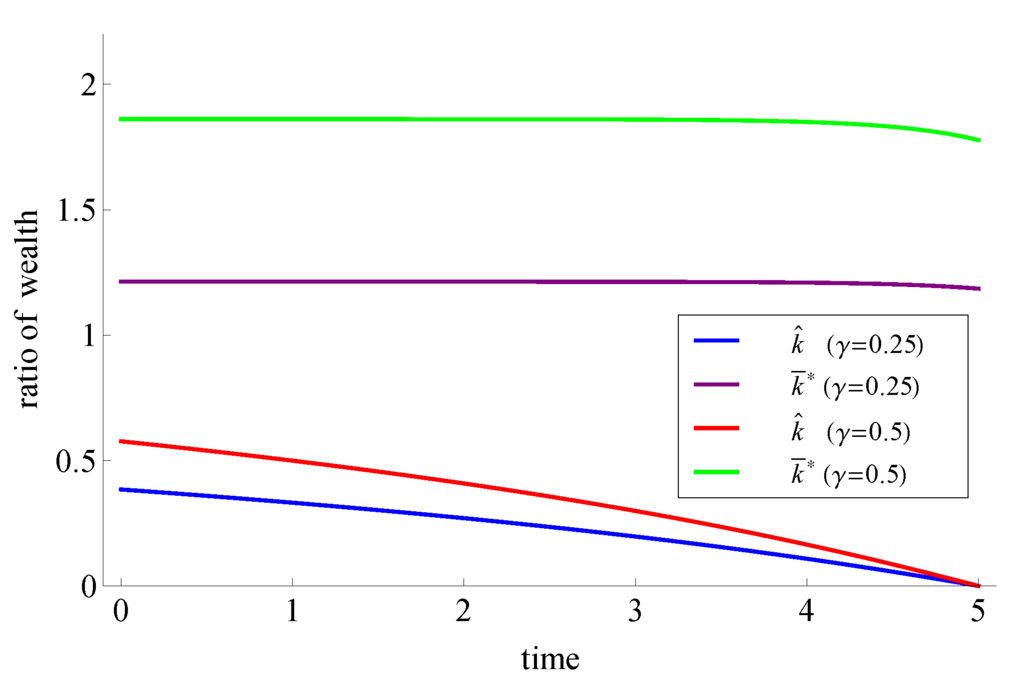
Figure 1. Optimal pre- and post-crash strategies for $\rho =0.5.$

Figure 1. Optimal pre- and post-crash strategies for $\rho =0.5.$

The same is true for the examples in Figure 2, where $\rho =-0.5$, $\gamma =-0.5$ and $\gamma =-3$. Analogously to the case of a constant interest rate, we can see that the optimal strategies before the market crash are lower for higher rates of relative risk aversion $1-\gamma$. Note that for the case $\gamma ·\rho \ge 0$, we have that the optimal pre-crash strategy is given by the indifference strategy. This result was already stated for models with a constant interest rate (see, e.g., [6]).

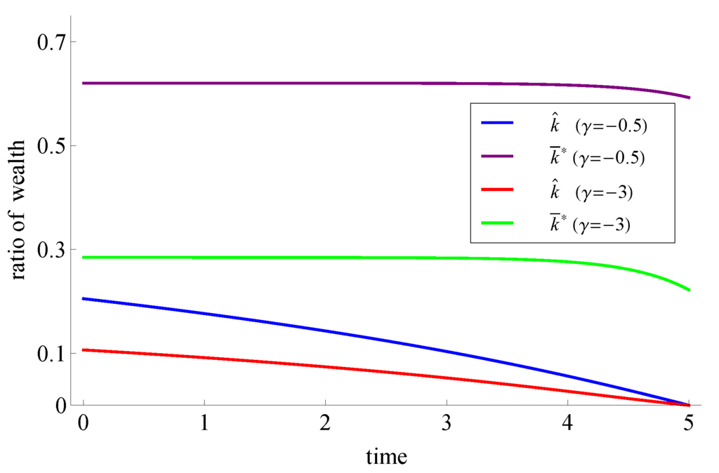
Figure 2. Optimal pre- and post-crash strategies for $\rho =-0.5.$

Figure 2. Optimal pre- and post-crash strategies for $\rho =-0.5.$

Now, if $\gamma ·\rho <0$, it can happen (depending on the choice of parameters) that ${\overline{k}}_t^{*}<{\widehat{k}}_t$ for some $t\in [0,T]$. In Figure 3, for example for $\rho =0.5$ and $\gamma =-13$, it is not optimal to follow the indifference strategy before the market crash. Indeed, the investor has to follow the post-crash strategy ${\overline{k}}_t^{*}$ for $t\in [0,t_S]$, where $t_S$ denotes the intersection point of ${\overline{k}}_t^{*}$ and ${\widehat{k}}_t$. Only after $t_S$, he will follow the indifference strategy ${\widehat{k}}_t$. Note that, due to the high rate of relative risk aversion ($1-\gamma =14$), the investor invests at most 0.02% of his wealth in the risky asset before the market crash occurs. If the market crash occurs before time $t_S$, he will stay at the post-crash strategy for all $t\in [0,T]$.

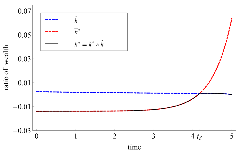
Figure 3. Optimal pre- and post-crash strategies for $\rho =0.5$ and $\gamma =-13$.

Figure 3. Optimal pre- and post-crash strategies for $\rho =0.5$ and $\gamma =-13$.

6. Conclusions and Outlook

Our main result, Theorem 2, provides a closed form solution of the worst-case optimization problem in (2) under a stochastic interest rate. The pre-crash strategy is given by the minimum of the indifference strategy and the post-crash strategy. For the case $\gamma ·\rho \ge 0$, we were able to show that the indifference strategy is smaller than or equal to the post-crash strategy for all $t\in [0,T]$, which implies that it is optimal to follow the indifference strategy before the crash. If $\gamma ·\rho <0$, it can happen, depending on the choice of market parameters, that it is optimal to follow the post-crash strategy first and, afterwards, to follow the indifference strategy. Due to the stochastic interest rate, we obtained that worst-case optimal strategies can also include short selling periods if the rate of relative risk aversion is sufficiently high.

There are various aspects that can be examined starting from our work. Among them are:

• The use of other interest rate models, such as the Cox–Ingersoll–Ross model or multi-factor models.
• Changing market parameters after the market crash.
• A market with at most n possible crashes.
• A multiple asset market.

A particularly interesting case can be the introduction of a more complicated jump behavior at the crash time. By this, we mean that both the stock price and the interest rate jump simultaneously.

References

- R.C. Merton. “Lifetime Portfolio Selection under Uncertainty: The Continuous-Time Case.” Rev. Econ. Stat. 51 (1969): 247–257. [Google Scholar] [CrossRef]
- R. Korn, and P. Wilmott. “Optimal portfolios under the threat of a crash.” Int. J. Theor. Appl. Financ. 5 (2002): 171–187. [Google Scholar] [CrossRef]
- R. Korn, and O. Menkens. “Worst-case scenario portfolio optimization: A new stochastic control approach.” Math. Methods Oper. Res. 62 (2005): 123–140. [Google Scholar] [CrossRef]
- R. Korn, and M. Steffensen. “On worst-case portfolio optimization.” SIAM J. Control Optim. 46 (2007): 2013–2030. [Google Scholar] [CrossRef]
- F. Seifried. “Optimal investment for worst-case crash scenarios: A martingale approach.” Math. Oper. Res. 35 (2010): 559–579. [Google Scholar] [CrossRef]
- R. Korn, and F.T. Seifried. “A Worst-Case Approach to Continuous-Time Portfolio Optimisation.” Radon Ser. Comput. Appl. Math. 8 (2009): 327–345. [Google Scholar]
- S. Desmettre, R. Korn, and F. Seifried. “Lifetime consumption and investment for worst-case crash scenarios.” Int. J. Theor. Appl. Financ., 2014. accepted. [Google Scholar] [CrossRef]
- R. Korn, and H. Kraft. “A stochastic control approach to portfolio problems with stochastic interest rates.” SIAM J. Control Optim. 40 (2001): 1250–1269. [Google Scholar] [CrossRef]
- O. Vasicek. “An equilibrium characterization of the term structure.” J. Financ. Econ. 5 (1977): 177–188. [Google Scholar] [CrossRef]
- T. Engler. “Worst-case optimization for an investment consumption problem.” In Proceedings of the Actuarial and Financial Mathematics Conference. Edited by M. Vanmaele, G. Deelstra, A. de Schepper, J. Dhaene, W. Schoutens, S. Vanduffel and D. Vyncke. Brussels, Belgium: Koninklijke Vlaamse Academie van België voor Wetenschappen en Kunsten, 2014, pp. 29–40. [Google Scholar]
- C. Jonek. “Stochastische Steuerung von Sprung-Diffusionen mit Anwendung in der Portfoliooptimierung.” Ph.D. Thesis, Heinrich-Heine-Universität Düsseldorf, 2008. [Google Scholar]
- D. Revuz, and M. Yor. Continuous Martingales and Brownian Motion. A series of comprehensive studies in mathematics; Heidelberg, Germany: Springer, 1999. [Google Scholar]
- P. Protter. Stochastic Integration and Differential Equations. Applications of Mathematics (New York); Berlin, Germay: Springer-Verlag, 1990, Volume 21. [Google Scholar]
- J. Prüss, and M. Wilke. Gewöhnliche Differentialgleichungen und Dynamische Systeme. Basel, Switzerland: Birkhäuser/Springer Basel AG, 2010. [Google Scholar]
© 2014 by the authors; licensee MDPI, Basel, Switzerland. This article is an open access article distributed under the terms and conditions of the Creative Commons Attribution license (http://creativecommons.org/licenses/by/4.0/).