Abstract
This paper studies the joint distribution of the default and prepayment losses for a large portfolio of loans, based on a bottom-up approach. The repayment behaviors of loans in the portfolio are determined by both systematic and idiosyncratic risk factors and are conditionally independent given the systematic factors. The joint two-dimensional limit distributions of the portfolio default and prepayment losses are obtained, including the strong law of large numbers and the central limit theorem. A numerical study for the portfolio losses is performed for some simplified models. Finally, we conduct the empirical analysis on the residential mortgage-backed security (RMBS) based on Freddie Mac’s dataset. The empirical results reveal the impacts of different factors on the default and prepayment behaviors, and the distributions of the portfolio losses are simulated based on empirical estimation results to show its difference with the log-normal distributions.
1. Introduction
For individual customers, a mortgage and personal loan are two common options for borrowing money from the financial institutions. A mortgage is a secured loan typically used for real estate financing, while a personal loan is an unsecured loan and can be flexibly used for various purposes. If the borrower fails to repay the mortgage, the lender has the right to foreclose the loan and repossess the property. The repayment process of a given loan may be subject to both default risk and prepayment risk. Default occurs when the borrower lacks sufficient funds to meet their debt obligations, or when the property value falls below the outstanding loan balance, potentially leading to a strategic default. Prepayment may occur, for instance, when there is a drop in the market interest rates, allowing the borrower to pay off the existing loan and refinance at a lower rate. Our study focuses on a large number of similar loans, which can be pooled and securitized as a portfolio for investing and trading, e.g., an asset-backed security (ABS) consisting of a specific pool of underlying loans. The total loss of portfolio includes default loss and prepayment loss, which come from the potential losses of each loan in the pool.
In early periods, the literature on modeling the loan for individual customers mainly focused on either default or prepayment. For example, in applying the option pricing models to mortgage defaults, Cunningham and Hendershott (1984) and Epperson et al. (1985) priced the default as a put option. The motivation is that the default occurs if the house price falls sufficiently below the mortgage value so that the decision of default follows a similar manner as the exercise of a compound European put option. Under the option pricing framework, Foster and Van Order (1984) and Quigley and Van Order (1995) empirically estimated the default models. In contrast, Dunn and McConnell (1981), Buser and Hendershott (1984), and Brennan and Schwartz (1985) priced the mortgages with prepayment risks by using the option-based approach. The introduction of the option pricing method lies in the fact that the prepayment gives the option to buy the remaining part of the loan (including the outstanding debt and prepayment cost) and therefore can be interpreted as an American call option on a bond. The estimation of prepayment models can be found in Schwartz and Torous (1989) and Quigley and Van Order (1990).
Since the 1990s, a number of works jointly modeled the default and prepayment as competing risks for the personal loan or mortgage. Deng et al. (1996) and Deng et al. (2000) extended the traditional option models to jointly consider default and prepayment as dependent risks in a proportional hazard framework for mortgages. Banasik et al. (1999) introduced the competing risks approach of survival analysis to study the prepayment and default for personal loans, where the applications of Cox’s proportional hazard (CPH) model were further extended by Stepanova and Thomas (2002). In later extensions, Quercia and Spader (2008) applied the multinomial logit model to investigate the homeownership education and counseling completion on the prepayment and default. Steinbuks (2015) studied the effect of prepayment penalty restrictions on the probability of prepayment and default. Zhang et al. (2019) proposed a mixture cure PH model under competing risks for an online loan. Some techniques for estimating the competing risks models include, e.g., a maximum likelihood technique based on constrained optimization in Thackham and Ma (2022) and a nonparametric life-table method in Li et al. (2023).
The existing research on the limiting portfolio loss mainly focused on default losses. Vasicek (1991) initiated this field by deriving the asymptotic distribution of portfolio credit losses under a single-factor Gaussian copula model. Credit Suisse Financial Products (1997) introduced a Poisson mixture model framework for analyzing the limiting portfolio loss. Gordy (2003) developed a single-factor model for the limiting loss of homogeneous portfolios, providing the theoretical basis for regulatory capital framework under Basel II/III.1 Giesecke et al. (2015) derived a law of large numbers for default losses in heterogeneous portfolios using the stochastic PDE methods. Sirignano and Giesecke (2019) proposed data-driven asymptotic approaches for the large loan pools, demonstrating their computational efficiency in computing the distributions of default rates, prepayment rates, and loss from default. In the industry, the top-down approach has been widely used to assess the limiting portfolio loss, focusing on directly modeling the distribution of total portfolio loss (e.g., the log-normal distribution for modeling the default loss in Moody’s Investors Service 2024).
In this paper, we model the limiting loss distribution for a large portfolio of loans by considering both default and prepayment risk as competing events (i.e., only the first occurred event is observed) and apply the model to a specific loan dataset. Our framework adopts a bottom-up approach to start by modeling the repayment behaviors of individual loans. At each discrete payment date, the repayment of a loan may end with either one of the three events: scheduled repayment completion, default, or prepayment. Building on this structure, we develop a joint model for the probabilities and loss values of both default and prepayment. The repayment behaviors of all the loans are determined by both systematic and idiosyncratic factors and are conditionally independent given the systematic factors. Under certain regular conditions, the limit properties of portfolio loss are discussed, including the strong law of large numbers (SLLN) and the central limit theorem (CLT). Further, we conduct an empirical analysis to estimate the probabilities of default and prepayment by applying the data of residential mortgage-backed security (RMBS). Based on the estimation results, we simulate the portfolio loss distribution, which is close to the log-normal distribution.
Our main contributions can be summarized as follows.
(a) We propose a discrete-time bottom-up portfolio loss model incorporating both default and prepayment risks. It is different from the existing frameworks for default losses in the single-period (Gordy 2003) or continuous-time (Giesecke et al. 2013) contexts. Several illustrative examples demonstrate that our discrete-time structure better captures the individual loan repayment behaviors, such as the monthly scheduled repayments and periodic event observations.
(b) Given the conditional independent structure, we investigate the limit properties of portfolio loss as the pool size tends to infinity, including the SLLN and CLT along with an upper error bound for approximating. Especially, under the assumption that the frequency of individual factors converges to a given distribution, the SLLN and CLT show that the limiting loss distribution of the portfolio is determined only by the systematic factors. We further verify this result by the numerical simulations of simplified models and find that the limiting distribution is approximately log-normal. Moreover, the copula of default and prepayment loss distributions are exhibited.
(c) Our empirical analysis applies the proposed framework to the empirical data, employing a CPH model to estimate the factor coefficients and baseline hazards. The estimated coefficients in the CPH model indicate that the systematic factors significantly influence both hazards. In terms of the influence of individual factors, the default risk is affected by loan-level credit quality, and the prepayment risk mainly depends on refinancing capacity. The out-of-sample validation reveals the good predictive performance of the model, and the estimated loss distribution is consistent with the CLT result. These findings align with the established theoretical and empirical evidence (see Calhoun and Deng 2002; Campbell and Cocco 2015). Finally, we perform the Monte Carlo simulation of portfolio default and prepayment losses based on the empirically estimated parameters. The asymptotic portfolio loss distributions display reasonable agreement with the log-normal distribution, which complies with Moody’s methodology (Moody’s Investors Service 2024).
The rest of this paper is organized as follows. Section 2 introduces the portfolio loss model considering both default and prepayment risk. Section 3 derives the limit properties of loss distribution under the conditional independent structure. Section 4 presents the empirical work and a further simulation study. Section 5 concludes.
2. The Portfolio Loss Model Considering Default and Prepayment
In this section, a general model is proposed for a portfolio of loans, where the repayment processes are exposed to both default risk and prepayment risk. The repayment behaviors of all loans are independent conditional on some common systematic factors, and each loan is also affected by some extra idiosyncratic factors.
2.1. The Portfolio Loss for a Pool of Loans
Building on the highly diversified characteristics of loan pools, we specify a general portfolio loss model that reflects the collective behavior of underlying assets. Assume that there are N unit-principal loans in the asset pool, which are issued at the same time and repaid periodically. For simplicity, the common scheduled periodical repayment dates of all loans are denoted as , where is the terminal time.
During the loan repayment process, the default or prepayment may occur on each loan. For the ith loan, let and be its time of potential default and time of potential prepayment, respectively. Since the default and prepayment are mutually exclusive, we assume that they do not simultaneously happen.
Assumption 1.
a.s., .
Based on the potential event times , define
Here, represents the time-until-termination, which is default at , prepayment at , and normal repayment at . A model for belongs to the class of multiple decrement models (see, e.g., Deshmukh (2012) and Chapter 7.2 of Rotar (2014)). For the ith loan, denote by and the loss given default and loss given prepayment, which are random variables taking values in . Then, the discounted default loss and prepayment loss at time 0 are defined as
respectively, where r is the constant risk-free interest rate. Denote by the ith loss vector. Then, the portfolio loss vector for the mortgage pool of N loans is given by
where represents the portfolio default loss and represents the portfolio prepayment loss, respectively. Throughout this paper, bold symbols are used for (column) vectors.
In practice, loans are classified as defaults only after a period of delinquency or inactivity. While some studies model the delinquency stages when analyzing the repayment behavior, our analysis mainly focuses on the terminal loss outcomes (default/prepayment). Since the observed default losses include those incurred during the delinquency periods, we adopt a single-step default framework for simplicity.
Remark 1.
We develop a discrete-time multi-period model, which naturally incorporates discounting by the risk-free interest rate. Notably, when , the model reduces to a single-period framework where we can set (i.e., no discounting), making it consistent with many classical single-period models in the literature (i.e., Gordy 2003; Vasicek 1991).
2.2. The Correlation Structure for the Portfolio Loss
In the following, we assume that the cash flow of payments for the N loans are influenced by some common systematic and macroeconomic factors , e.g., refinancing interest rate, GDP growth rate, unemployment rate, and industry-performance factors, which can vary through time. For , the repayment behavior of the ith loan is also determined by some extra idiosyncratic factors , which remain unchanged through time. Here, have the same category and dimension. For example, Sirignano et al. (2016) and Sirignano and Giesecke (2019) consider the credit score, LTV ratio, initial loan rate, type of loan, collateral type, and geographic location as the individual factors. Regarding the factors and , we make the following two assumptions.
Assumption 2.
For , , and , there exist continuous functions , , and such that
Assumption 3.
The N random vectors are mutually independent conditional on .
Assumption 2 means that the loss probabilities of the ith loan are fully determined by the individual factors and systematic factors . Given , the repayment behavior of the ith loan is illustrated in Figure 1. At each time , the ith loan is exposed to the default risk and prepayment risk, with the probability of default and the probability of prepayment. Although the actual loss values are not uniquely determined by the individual factors and systematic factors , the first and second moments of the loss distribution (equivalently, its expectation and variance) are fully specified by these factors.
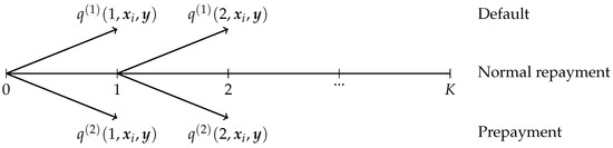
Figure 1.
The repayment behavior of the ith loan.
Assumption 3 implies that the repayment behaviors of the N loans are independent conditional on the systematic factors , which is a standard modeling approach in the literature (see Credit Suisse Financial Products 1997; Gordy 2003). Note that for some , the components in need not be conditionally independent.
Some commonly used models for in the literature are listed in Example 1.
Example 1.

Three different models for are presented in Table 1. While the predictions of default and prepayment probabilities for the linear regression model may fall outside the range , this limitation is resolved by the subsequent use of the multinomial logistic model (Calhoun and Deng 2002). Additionally, the proportional hazard model incorporates the baseline hazard functions , which capture the time-dependent structure of the baseline risk for each event j at the time period k.
Table 1.
Some models for in the literature.
Moreover, some widely used models for , , and in Assumption 2 are given below.
Example 2.
Assume that each loan is repaid by equal installments. For the ith loan, denote by its fixed loan rate, the fixed periodic payment for K periods, and the outstanding balance at time k, . By the discounted cash flow formula,2 we have
Note that is one of the individual factors in , so both and in (7) are functions of .
For the ith loan, the default loss at time k is a percentage of the outstanding balance (Flores et al. 2010). As modeled in Moody’s Mortgage Portfolio Analyzer (MPA) methodology (Stein et al. 2011), the loss at time k is given by
conditional on , where is a Beta-distributed ratio of loss given default (LGD) with parameters and . Consequently, we have
and
Alternatively, the prepayment losses are determined by interest rate differentials (Jones and Chen 2016; Richard and Roll 1989). For the ith loan, the prepayment loss at time k is given by
conditional on , where represents the risk-free discounted value of the unpaid balance at time k, and is the outstanding loan balance in (7). Consequently, we have with in (8).
Denote
In the following, we derive some results for the conditional distribution of defined in (1).
Lemma 1.
Suppose that Assumptions 1–3 hold.
- (i)
- (ii)
- The conditional joint distribution of is given bywhere is defined in (4).
For later use, below we derive the expectations and variances of and conditional on , as functions of , , and . For convenience, define
with
Proposition 1.
Proposition 1 lays a basic setup for deriving the limit distributions in Section 3. Some specific models are introduced in Section 3.3.
Remark 2.
To better reflect the influence of default and prepayment behaviors, when calculating the discounted loss amounts from default and prepayment in Proposition 1, we employ a constant market interest rate. The extensions to the context of stochastic interest rate can be also similarly considered.
3. The Limiting Distribution of the Portfolio Loss
In this section, we study the limit properties of the portfolio loss as , including the law of large numbers, the central limit theorem, and an upper bound on the error term. For technical uses, two assumptions are introduced below.
Assumption 4.
There exists a distribution function , such that
where “” means the weak convergence.
Assumption 5.
There exists some , such that a.s., .
Assumption 4 characterizes the limiting behavior of the frequency counts of individual factors in the mortgage pool. Aligning conceptually with Assumption 2.2 of Giesecke et al. (2013) and Condition 2.1 of Giesecke et al. (2015), it implies that as the pool size grows, the distribution of these factors converges to a simpler macroscopic characterization. This assumption allows us to model the overall features of the portfolio instead of focusing on the individual data characteristics under the large-sample context.
Assumption 5 imposes a lower bound on the determinant of the covariance matrix . This condition rules out some degenerate scenarios by ensuring that (i) both default loss and prepayment loss exhibit non-trivial variability (i.e., their variances are bounded away from zero) and reflect the realistic fluctuations in loan portfolios; (ii) the losses are not perfectly linearly dependent, excluding the artificial cases where one loss becomes completely predictable given the other; and (iii) the joint distribution maintains a genuine two-dimensional randomness structure, preventing pathological concentration of risk. This mathematical formulation effectively captures the natural dispersion and imperfect dependence between default and prepayment behaviors observed practically.
3.1. The Strong Law of Large Numbers
First, the strong law of large numbers on as is provided. For ease of exposition, define
with and given in (11), and introduced in Assumption 4. For later use, denote and .
Proposition 2.
Suppose that Assumptions 1–3 hold. Let be as in (3).
Intuitively, Proposition 2 (i) states that for a portfolio with a large number of individuals, converges to its conditional expectation. Note that in (15) is determined by both systematic factors and individual factors . Compared to (i), Proposition 2 (ii) establishes a simpler, almost sure limit of in terms of the limit distribution . As shown in (19), the limit depends only on the vector of systematic factors , which requires less underlying information and provides greater computational efficiency via the simplified expression.
Recall that . The following examples demonstrate some straightforward applications of Proposition 2 to the cases where the dimension of is one or two.
Example 3.
(i) Suppose that is a one-dimensional random variable (denoted by Y), is a continuous increasing function, and is a continuous decreasing function. Then, we have
and
where is the distribution function of Y. In this setting, and nearly exhibit the counter-monotonicity as . This is because the limit of increases in Y, while the limit of decreases in Y.
(ii) Suppose that is a two-dimensional random vector and is a continuous differentiable bijection. Then, the limit of probability density function of as can be approximated by
where denotes a vector satisfying .
For a random variable X, the VaR of X at level is defined as . The result (19) leads to the following corollary on the VaR of as .
Corollary 1.
Suppose that Assumptions 1–4 hold. For any and , we have
and
Given Corollary 1, the VaR of can be applied to approximate the VaR of for large N.
3.2. The Central Limit Theorem
In the following, a central limit theorem (CLT) is provided for in (3). Denote by the identity matrix. For a positive-definite matrix A, is defined as its inverse square root via spectral decomposition; see the footnote for details.3
Theorem 1.
Suppose that Assumptions 1–3 and 5 hold.
Similar to Proposition 2, and in Theorem 1 (i) include the information of both systematic factors and individual factors , while and in Theorem 1 (ii) are only determined by and the asymptotic distribution . The simplified expression in (ii) reduces the data requirements while enhancing the computational efficiency.
Based on Theorem 1, the following corollary further studies the CLT on the default loss , the prepayment loss , and the total loss . Recall that .
Corollary 2.
Suppose that Assumptions 1–5 hold. Then, conditional on , we have
and
as .
Corollary 2 follows directly from Theorem 2.3 in Van der Vaart (2000) on preserving the asymptotic normality under linear transformations. The proof is therefore omitted.
Theorem 1 (i) implies that conditional on , the distribution of portfolio loss with large number N can be approximated by the normal distribution . Denote by the distribution function of and is the distribution function of normal distribution . Then, the joint distribution of can be approximated by
Moreover, the error term in approximation (23) admits an explicit upper bound, as presented below.
Theorem 2.
Suppose that Assumptions 1–3 and 5 hold. The error term in (23) is bounded by
with ε introduced in Assumption 5.
Theorem 2 implies that the error term for the distribution function of converges to zero at the rate .
3.3. Numerical Analysis for Some Models
Under certain assumptions, the limiting portfolio loss follows the SLLN in Section 3.1 and CLT in Section 3.2, respectively. Specifically, Proposition 2 states that the portfolio loss can be approximated by in (19). However, sometimes it is difficult to calculate due to the large number of parameters in and the complexity of the expressions involved in . Hence, this part introduces two simplified models, where can be directly represented.
3.3.1. The Asset Value Model
The asset value models introduced by Merton (1974) and Finger (1999) are widely used in the industry, where the loan’s repayment behavior is determined by its underlying asset value (or return rate). Based on the repayment solvency considerations, we assume that the default occurs when the asset value falls below a predetermined threshold, while the prepayment is triggered when the asset value exceeds a higher threshold. For simplicity, we abstract away from temporal dynamics and consider a single-period setting ( and ).
In this model, the vector consists of n market factors, jointly following a standard multivariate normal distribution . The vector comprises the n coefficients (sensitivities) of the ith borrower to these market factors. The return rate is defined as
where are idiosyncratic performance terms independent of . Let and denote the critical thresholds for default and prepayment, respectively, defined in terms of the return rate. In this case, the probabilities of default and prepayment for the ith loan are given by
For simplicity, assume the default loss is the constant and the prepayment loss is the constant . Then, we obtain from (12). Building on the Equation (17), the entries of can be expressed as
3.3.2. The Markov Model
Consistent with the transform mechanism of the Markov model (see Jarrow et al. 1997), we assume that the probabilities of default and prepayment are fixed during the payment period, i.e., for , . Specifically, it follows the multinomial logistic model given by Example 1:
For simplicity, we assume the default and prepayment losses are proportional to the remaining repayment period, expressed as
for . This linear scaling implies that losses decrease uniformly over time. We do not assume the special forms of and in Assumption 4. Under this setup, the functions , defined in (12) have the following specific form.
Subsequently, the function is given by (21) with specified in Lemma 2.
3.3.3. Simulation Results
Based on the simplified theoretical loss models, we conduct the Monte Carlo simulations to analyze the loss distributions and compare them with the log-normal distribution proposed by Moody’s Investors Service (2024). For each model, we perform the simulations with a portfolio of 10,000 loans and 10,000 Monte Carlo trials. The key parameters include the payment periods K, the risk-free interest rate r, the distribution of and in Assumption 4, and the functions and in Assumption 2. These parameters are provided differently in the models of Section 3.3.1 and Section 3.3.2. The simulation takes the following steps.
- (i)
- The individual and systematic factors. First, we generate the individual factors from the distribution and fix them in the subsequent steps. Then, in each simulation, we generate the systematic factors from the distribution , representing an economic scenario.
- (ii)
- The repayment behaviors. Given the factors and in each simulation, the repayment behaviors are simulated as in Figure 1, with default/prepayment rates , . For simplicity, the default/prepayment losses are fixed at their expected values .
- (iii)
In the following, denote the distribution function of the Beta() distribution by
Based on the asset value model, Figure 2 presents the simulations for the limit distribution of portfolio loss under different parameter settings. The main parameters are set based on the existing literature. The default rates and align with the B-rated bond studies ( in Frey and McNeil (2003), in Gordy (2003), and in Credit Suisse Financial Products (1997)), while the prepayment rates were assumed based on Deng et al. (2000). Since the loan recovery rate are set as , and in Credit Suisse Financial Products (1997) for different seniority levels and securities, we adopt and , respectively, in Figure 2. Some other parameters are set according to the asset correlations derived from Flores et al. (2010), while the rest of the parameters were selected for the purpose of simulation.
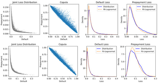
Figure 2.
The joint distribution, copula, and marginal distributions of for the asset value model. Note: The upper panel and lower panel exhibit the joint distribution, copula, and marginal distributions of for two cases of the asset value model in (24) and (25), respectively. In the upper panel, we set , , , , , , and . In the lower panel, we set , , , , , , and .
The results in Figure 2 show the clear negative correlation between the loss of default and the loss of prepayment. The empirical distributions of both default and prepayment losses in the simulated data show strong agreement with the log-normal distributions. Furthermore, the loss distribution exhibits a unimodal pattern, peaked at relatively small loss values and decreasing monotonically as the losses increase.
Under the above Markov model, Figure 3 presents the simulations illustrating the distribution of portfolio loss under different parameters. The parameter selection is similar to that in Figure 2. The results show that the marginal distributions of fit the log-normal distribution well and further validate the log-normal assumption in Moody’s methodology (Moody’s Investors Service 2024).
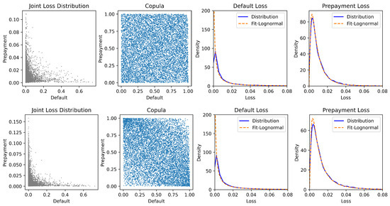
Figure 3.
The joint distribution, copula, and marginal distributions of for the Markov model. Note: The upper panel and lower panel exhibit the joint distribution, copula, and marginal distributions of for two cases of the Markov model in (26) and (27), respectively. In both cases, we set , , , , and . The upper panel corresponds to , , and . The lower panel corresponds to , , and .
4. Empirical Studies
In this section, we present an empirical analysis of the residential mortgage-backed security (RMBS) under our setup of jointly modeling the default and prepayment. As a type of ABS, the RMBS is created by pooling numerous residential mortgage loans and converting them into tradable investment instruments. The investors can invest into the RMBS according to their personal risk preferences. Nowadays, the RMBS stands as the largest proportion of the cash securitization market globally, especially popular in the US, continental Europe, the UK, Australia, etc.4
The residential mortgage loans in the RMBS typically exhibit distinct characteristics, such as fixed or adjustable interest rates, long-term maturities (e.g., 15–30 years), and amortizing payment structures. The RMBS is also exposed to the default and prepayment risks. The default is usually driven by borrower financial distress, declining property values, or macroeconomic shocks, leading to the credit losses. The prepayment is triggered by refinancing (e.g., rate declines) or home sales, altering the cash flow timing and reinvestment risk. The performances of residential mortgages in the RMBS are affected by a series of factors, including the borrower quality, underwriting guidelines, and servicer/originator quality.
As an application of our theoretical framework, the empirical study pursues two objectives. First, we incorporate both default and prepayment risks into the portfolio loss model of the RMBS and empirically investigate how the factors significantly affect the default and prepayment. Second, we use the estimated hazards to generate bottom-up Monte Carlo simulations of portfolio losses. Note that it is complex to represent the asymptotic conditional expectation of portfolio loss in Proposition 2. Our empirical results suggest that this conditional expectation of portfolio loss is approximately log-normally distributed, thereby enriching the theoretical model with distributional insight grounded in data.
The study employs Freddie Mac’s single-family loan dataset issued in 2000 and focuses on the 15-year mortgages with monthly repayments. The dataset with full origination and monthly performance records has become a benchmark source for mortgage credit studies (see, e.g., Goodman et al. 2014; Goodman and Zhu 2015; and Bhattacharya et al. 2019). Since this standard dataset consists solely of fixed-rate loans, we restrict the analysis to this loan type. The dataset of fixed year 2000 is selected to ensure a sufficiently long repayment observation period (up to 15 years/180 months as analyzed). Robustness checks confirm that the result does not depend on the choice of the year.
4.1. Model Setup for RMBS Product
With the notation introduced in Section 2, suppose that there are N mortgages in the pool of the RMBS, with the common repayment period of K months. For each mortgage, there are three mutually exclusive states in each month: default, prepaid, or active (normal amortization). The default and prepayment risks of an individual loan are modeled by the Cox proportional hazard functions, which depend on the systematic factors and the vector of individual factors fixed at the issue date.
4.1.1. Systematic Factors
The systematic factors represent a multivariate time series of macroeconomic variables. Denote the vector of systematic factors observed in the kth month by
The first component is the U.S. Treasury long-term yield rate and serves as the refinancing benchmark, which is distinct from the contractual loan rate set for individual borrowers. The difference captures the evolving interest rate spread that affects both prepayment for refinancing and default decisions. The symbols represent d administrative states in the U.S., so that each mortgage in the pool is located in some state. For , denotes the state-level house price changes (HPCs) in the state at the kth month and captures the house price dynamics, defined by
where is the house price index (HPI) for the state at the kth month. By collecting the systematic factors among , the obtained vector is random with the dimension .
4.1.2. Individual Factors
For the ith loan, the individual factors are collected as
where is the original loan rate, is the borrower’s credit score, is the loan-to-value ratio, is the debt-to-income ratio, is the indicator for first-time home-buyer (1 for yes and 0 for no), and is the number of borrowers on the loan. The final coordinate identifies the U.S. state where the property is located. This identifier links the ith loan to the time series of state-level house price changes .
Based on the systematic and individual factors, the competing risks (default and prepayment) are specified by the CPH model demonstrated in Table 1. The CPH framework is widely adopted in mortgage research and practice; see, for example, Deng et al. (2000), Li et al. (2023), and Moody’s Mortgage Portfolio Analyzer (MPA) methodology (Stein et al. 2011). Specifically, the probabilities of default and prepayment in (4) are given by
for . Here, is the baseline hazard function and captures the time profile of default or prepayment risk when all the explanatory factors are fixed at the neutral levels. The exponential term in (30) rescales the benchmark according to the individual characteristics of mortgages and prevailing macroeconomic conditions.
4.2. Freddie Mac Single-Family Loan Dataset
Our empirical analysis utilizes the complete Freddie Mac single-family loan dataset,5 which includes all available 15-year fixed-rate mortgages issued in 2000. We partition the data into a training set of 500,000 loans and a test set of 57,202 loans (the remaining parts outside the training set). Both sets are mutually exclusive and randomly selected, preserving the homogeneity. Crucially, our robustness checks confirm that the results also hold even when using only 500,000 randomly sampled loans (vs. the entire 557,202), which indicates that the sensitivity to dataset size or selection is small. The dataset comprises the loans from all 50 U.S. states, with the distribution among states illustrated in Figure 4. The largest share is from California (10.8%), followed by Florida (6.6%), Texas (6.4%), and Illinois (5.4%), and no other state exceeds 5%. The “Others” category aggregates smaller states, accounting for approximately half (54.2%) of the sample, highlighting that the dataset is broadly representative across the geographic regions without significant concentration. In sum, the dataset for estimation consists of loans with monthly repayments.
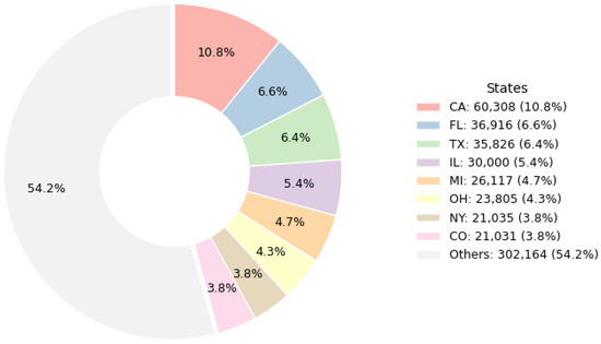
Figure 4.
Distribution of mortgages by state.
The loan status can be deduced from the variables “Zero balance code” and “Defect settlement date” in the dataset. With slight modifications from the definitions outlined in Bhattacharya et al. (2019) due to data updates, the default and prepayment are now defined as follows:
- A loan is considered default if, for any month, the “Zero balance code” falls within the set .
- A loan is considered prepaid if, for any month, the “Zero balance code” is equal to 01 and the “Defect settlement date” is “NAN”.
- A loan remains active if it does not meet the criteria for prepayment or default.
As described in Section 4.1, the systematic factors in our study are the U.S. Treasury long-term yield6 available at a monthly frequency, and the quarterly state-level HPI data,7 from which we compute the house price changes . The quarterly HPI data are linearly interpolated to a monthly frequency. The individual factors (i.e., loan rate, CS, LTV, DTI, FTB, and NB) are directly extracted from the dataset, which are fixed at the mortgage issue date.
To derive the loss value of the RMBS, the LGD of defaulted loans are obtained via the variables “Actual Loss Calculation” and “Current Actual UPB” from the dataset,
Those observations outside the interval are discarded.
4.3. Estimation Results
4.3.1. The Coefficients of Factors
Based on the training data of 500,000 mortgages issued at year 2000 (to year 2015) in the Freddie Mac dataset, the coefficient vectors in the joint default–prepayment hazard model (30) are estimated by the maximum partial likelihood method, where the details of the methodology are provided in Appendix B.1. The estimation results are shown in Table 2 and provide some empirical evidence to explain the effect of different factors on the default and prepayment.
Table 2.
The coefficient vectors of the CPH model.
First, the borrower behavior is strongly influenced by the market-level systematic factors. Specifically, higher interest rate spreads encourage the borrowers to refinance or sell, substantially increasing the voluntary prepayment; however, the borrowers who are unable to refinance experience greater financial pressure, which leads to higher default risk. Further, the rising house prices enhance the borrower equity, improving the incentives to maintain ownership, thus lowering the default risk (reflected by the negative coefficient of HPC). Conversely, the rising house prices provide easier refinancing opportunities and profitable property sales, increasing the prepayment probabilities (reflected by the positive coefficient of HPC). These findings align with the existing literature (Campbell and Cocco 2015; Quercia and Stegman 1992).
Second, the borrowers’ credit quality and financial structure play a critical role in determining the default risk. Higher credit scores, first-time buyers, and the presence of co-borrowers are associated with significantly lower default probabilities, as indicated by their negative coefficients, reflecting the stronger repayment capabilities and reduced financial distress. In contrast, the single-borrower households demonstrate greater vulnerability to financial distress, leading to elevated default rates. Additionally, higher LTV ratios significantly increase the default risk by reducing the equity buffers and intensifying the financial pressure for borrowers.
Third, the prepayment behavior is accelerated primarily by the stronger refinancing capacity of borrowers. Specifically, the borrowers with higher CS, DTI, and NB prepay more rapidly, reflecting the greater incentives and ability to refinance or sell. This is consistent with the related analysis of prepayment in Munk (2011). In contrast, the prepayment rate is insensitive to the LTV ratio and FTB status.
In summary, the estimation results show that the default and prepayment behaviors of borrowers are affected by distinct economic factors. This can improve the understanding of RMBS loan performance and leads to more accurate portfolio loss forecasts.
4.3.2. Baseline Hazard Functions
Based on the estimated coefficients in Equation (30), we estimate the baseline hazard functions by matching the expected event numbers with the actual data. The details of the methodology are provided in Appendix B.2. The estimation results for default and prepayment are plotted in Figure 5. The prepayment hazard rate peaks in the first 60 months and flattens from then. The default rate is much lower than the prepayment rate and presents a smoother curve.
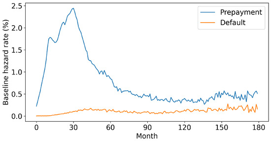
Figure 5.
The baseline hazard functions.
These patterns have important implications for modeling the borrower behavior and predicting the RMBS cash flows. The significantly higher prepayment risk in the early life of loans underscores the need to capture the time-varying characteristics of the interest rate, which has an influence on the borrowers’ refinancing incentives. On the other hand, the relatively smooth and lower default hazard suggests that the borrowers’ default behaviors are relatively rare and often occur uniformly over time rather than present the clustering characteristics as the prepayment.
4.3.3. The Distribution of LGD
To incorporate the borrower credit quality heterogeneity into the loss severity, we partition the loans into three categories based on the CS percentiles. Specifically, the top of loans ordered by CS are labeled as the high credit score borrowers, the middle as the moderate, and the bottom as the low. For each group, we estimate the LGD distribution by fitting the observed loss data derived by (31) to the Beta distributions, following Moody’s RMBS methodology (Moody’s Investors Service 2024). Table 3 reports the mean of the LGD and the corresponding Beta distribution parameters for each category.
Table 3.
The LGD distibutions for different categories of credit scores.
As shown in Table 3, the borrowers with higher credit scores tend to have lower LGD. Incorporating this classification into the simulation allows for more accurate modeling of loss severity across heterogeneous credit risk profiles.
4.3.4. Out-of-Sample Validation
To check the robustness of the estimation procedure, we conduct an out-of-sample validation using a separate test set consisting of 57,202 loans issued in 2000. Figure 6 compares the model-implied cumulative defaults and prepayments against the actual observed values in this test set.
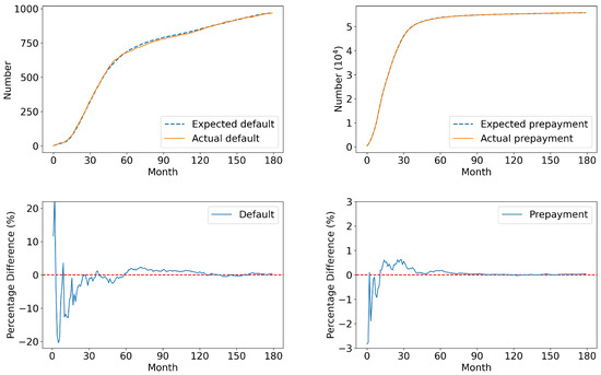
Figure 6.
The estimation results of default (left) and prepayment (right) in the test set. Note: the red dotted lines in the lower panels represent zero difference between the expected and actual number of defaults, serving as a baseline for comparing the percentage difference curves.
The close alignment between the estimated and realized outcomes indicates that the estimation procedure is effective. The estimation error is relatively larger in the first few months, primarily due to the limited number of early default/prepayment behaviors, which affects the statistical precision. Nevertheless, the errors decrease quickly over time, indicating that the model captures the underlying risk dynamics reasonably well. These results suggest that our framework is useful for accurately estimating the default and prepayment probabilities in modeling the RMBS, which are essential for further evaluating the portfolio losses.
With a realized systematic factor path fixed (see Appendix B.3 for details of the structure of ), we draw independent samples of the portfolio loss from the estimated CPH model. Figure 7 plots the empirical distributions of and together with the fitted Gaussian densities. The close visual agreement supports the conditional CLT in Theorem 1. The bivariate normal parameters estimated from the draws are
and the correlation coefficient is The negative correlation between default and prepayment losses reflects the competing-risk nature of these two events in the RMBS portfolios, where the early prepayment naturally reduces the number of loans exposed to default risk. This finding aligns with actual market behavior and highlights the importance of jointly modeling default and prepayment risks.
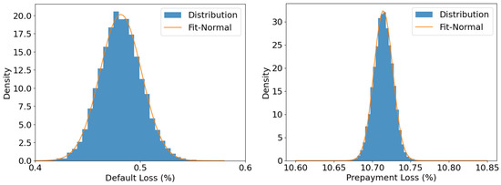
Figure 7.
Empirical limit distributions of default loss (left) and prepayment loss (right).
4.4. Simulation of Portfolio Loss
Recall that in Proposition 2 (ii), the portfolio loss converges to the conditional mean as , but the distributions of random variables and in do not admit explicit expressions. To further investigate the distribution of , in this part we generate the loss distribution of a representative RMBS pool using a bottom-up approach. Given the estimated hazard functions for default and prepayment from Section 4.3, we simulate the losses of individual loans based on the simulated dynamics of systematic risk factors. Then, the portfolio loss for the RMBS is generated.
4.4.1. The Models of Systematic Factors
In our model, both the interest rate and house price changes have influence over the payment period. To simulate the evolution of interest rates, we adopt the Cox–Ingersoll–Ross (CIR) model (Cox et al. 1985), which is widely used due to its ability to capture the non-negativity and mean-reverting nature of interest rates. The discrete-time approximation of the CIR process using the Euler–Maruyama scheme is given by
where is the time step ( for monthly frequency), is the mean of the long-term interest rate, is the rate of average recovery, is the volatility, and are i.i.d. random variables.
The parameters of the CIR model are estimated using the historical U.S. Treasury long-term yield data obtained from the U.S. Department of the Treasury. The estimated results are reported in Table 4. One sample path of the simulated interest rate over a 180-month period is shown in Figure 8. Here, the actual rate curve represents the observed U.S. Treasury long-term yield data from the historical record over the same period. The downward trend in the simulated interest rate arises naturally due to the mean reversion towards the estimated long-run equilibrium rate. As shown in Table 4, the initial historical rate exceeds the equilibrium value . The declining rates widen the loan spreads, subsequently elevating the default and prepayment probabilities and thereby increasing the potential portfolio losses.
Table 4.
The estimators of the CIR model.
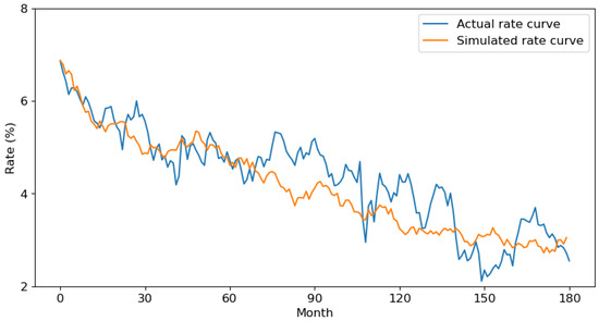
Figure 8.
A simulation of the interest rate curve.
To simulate the dynamics of the house price across the U.S. states, we employ a second-order autoregressive model (AR(2)) on the log house price index series. Specifically, for each state , the log house price index evolves according to
where , are i.i.d. standard normal shocks in the kth month. Subsequently, the HPC is calculated by the Equation (29).
The estimated AR(2) parameters of all U.S. states are summarized in Table 5. The last row of Table 5 reports the AR(2) estimates for the national-level log house price series, which provides a benchmark for comparing the state-level dynamics. The AR(2) simulations consistently reveal a persistent and autoregressive growth pattern, despite the different initial house price levels across states.
Table 5.
Summary statistics of AR(2) parameters for log house price time series across U.S. states.
4.4.2. Simulation Results
Based on the empirical results in Section 4.3, we simulate the RMBS portfolio losses under a bottom-up framework. In each scenario, we simulate one sample of the portfolio default and prepayment loss for the pool of 57,202 loans in the test set. By repeating this process over 100,000 times, we generate the distribution of and , where the marginal distributions for and are presented in Figure 9.
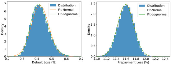
Figure 9.
The marginal distributions of the simulated portfolio loss of the RMBS.
From the right panel in Figure 9, both normal and log-normal distributions provide a good approximation for the distribution of portfolio prepayment loss. In contrast, as seen in the left panel of Figure 9, the log-normal distribution offers a substantially better fit of the portfolio default loss, compared to the normal distribution. This empirical observation provides quantitative evidence for the commonly assumed log-normal specification in the top-down models.
To further empirically examine the distributional form of and , we take the logarithm of the simulated portfolio loss and construct the quantile–quantile (QQ) plots against the normal distribution. As shown in Figure 10, the log of losses are close to the theoretical quantiles of a normal distribution, with only mild deviations in the tails. This evidence suggests that is approximately log-normally distributed under the simulated macroeconomic scenarios.
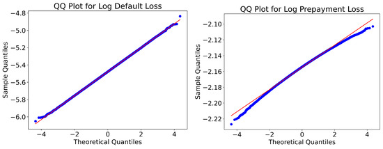
Figure 10.
The QQ plots for the simulated portfolio loss of the RMBS. Note: The blue line represents the empirical quantiles of the simulated data, while the red straight line corresponds to the theoretical quantiles of a normal distribution.
Moreover, the value-at-risk (VaR) of simulated and and the corresponding fitted log-normal distributions are shown in Table 6. The small deviations between the fitted and simulated values reveal that the log-normal distribution provides a reasonable approximation of the portfolio loss distribution. This result not only supports the log-normal assumption widely adopted in the top-down credit risk models but also fills an important gap in our theoretical framework by offering a plausible empirical distribution for the conditional loss mean.
Table 6.
The VaR of the simulated and of the RMBS.
5. Conclusions
This paper discussed the joint distribution of default and prepayment losses for a large portfolio of loans, extending the previous studies that focused solely on default losses. Under the conditionally independent framework, the two-dimensional limit distributions of the portfolio default and prepayment losses were obtained, including the strong law of large numbers and the central limit theorem. Numerical studies for the portfolio losses were performed for some simplified models. Empirical analysis on the RMBS was carried out for analyzing the limit joint distribution of the default and prepayment losses. The portfolio default and prepayment losses were simulated based on the empirically estimated model parameters. The copula of default and prepayment loss distributions was exhibited. Both the simulated distributions of portfolio default and prepayment losses fitted the log-normal distributions well, which is consistent with the log-normal distribution assumptions for portfolio losses in Moody’s Investors Service (2024).
Author Contributions
Conceptualization, methodology, formal analysis and investigation, C.X., X.Z., L.B., Q.D. and J.Y.; software, validation, data curation and visualization, C.X., L.B. and Q.D.; writing—original draft preparation and writing—review and editing, C.X., X.Z., Q.D. and J.Y.; supervision and funding acquisition, X.Z. and J.Y.; resources and project administration, J.Y. All authors have read and agreed to the published version of the manuscript.
Funding
This research was supported by the National Key R&D Program of China (Grant No. 2018YFA0703900) and the National Natural Science Foundation of China (Grant Nos. 12471445 and 12071016). The research of Zang was also supported by the National Natural Science Foundation of China (Grant No. 12301598).
Data Availability Statement
The data of the empirical study in this paper is obtained from the Freddie Mac single-family loan dataset released by the Federal Home Loan Mortgage Corporation.
Conflicts of Interest
The authors declare no conflicts of interest.
Appendix A. Some Proofs
Appendix A.1. Proof of Lemma 1
Appendix A.2. Proof of Proposition 1
Proof.
(i) Given , for , the conditional expectation of in (2) is given by
with defined in (12). Similarly, we get
which yields that
with defined in (13). Moreover,
where the last equality is due to , and thus, . So, conclusion (14) follows.
(ii) For in (3), we have
Moreover, by Assumption 3, are conditionally independent given . This yields
□
Appendix A.3. Proof of Proposition 2
Proof.
(i) From Assumption 3, the sequence is conditionally independent given . For , conditional on , the sequence
satisfies the conditions of Theorem 2.5.3 in Durrett (2019), such that they are conditionally independent with a conditional expectation of 0, and
where the first inequality follows from and further . Applying this theorem, we conclude that converges almost surely as conditional on . By Kronecker’s lemma (Theorem 2.5.5 in Durrett 2019), this implies
That is, in vector notation. Then, we have
which yields Equation (18).
(ii) Since the functions and in (4) are continuous, the moment functions defined in (11) are consequently continuous and bounded in [0,1]. Moreover, Assumption 4 establishes the weak convergence as . By the weak convergence theorem (Theorem 3.2.3 in Durrett 2019), we have
with defined in (17). Combining (18) and (A1), we obtain Equation (19). □
Appendix A.4. Proof of Corollary 1
Proof.
From Proposition 2 (ii), converges almost surely to as . Consequently, for , its component a.s. This implies convergence in distribution, i.e.,
for any continuity point t of .
Appendix A.5. Proof of Theorem 1
For the proof of this theorem, we first propose two technical lemmas.
Lemma A1.
For , let be a symmetric matrix of the form
for some . Define the sum matrix . Then, each entry of the inverse matrix is in the interval .
Proof.
For each , the determinant condition implies . Then, it follows that
where the last inequality is due to Cauchy–Schwarz’s inequality (see Theorem 4.1 in Rudin (1987)). Thus,
and . Note that
As all entries of matrix A, i.e., , and , are bounded in , each entry of matrix is bounded in , which finishes the proof. □
Lemma A2.
Suppose that Assumptions 1–3 and 5 hold. Given vector , define random variables
Then, , with ε in Assumption 5.
Proof.
Note that each entry of is in by definition (2). Further, from Assumption 5, the matrices , satisfy condition (A5). By Lemma A1, each entry of
is bounded in , where the equality is due to the conditional independence in Assumption 3. Moreover, since each entry of is bounded in , we have
for . This finishes the proof. □
Now, we prove Theorem 1.
(i) Given , the variables defined in (A6) are conditionally independent by Assumption 3 and satisfy , . Moreover,
where the second equality is due to (3) and the last equality follows by combining (15) and (21).
Note that
where the first equality is due to and the third equality is due to (A8). And for any ,
where the inequality follows from Lemma A2. Equations (A9) and (A11) satisfy the Lindeberg CLT conditions, see Theorem 11.1.6 in Athreya and Lahiri (2010). By this theorem, we achieve
which finishes the proof. □
(ii) As discussed in the proof of Proposition 2 (ii), the moment functions in (11) are continuous and bounded in [0,1], and the weak convergence (16) holds. By the weak convergence theorem (Theorem 3.2.3 in Durrett 2019), we have
with and defined in (17) and (21). Combining (20) and (A12), we obtain Equation (22).
Appendix A.6. Proof of Theorem 2
For the proof of this theorem, a technical lemma is proposed.
Lemma A3.
Suppose that Assumptions 1–3 and 5 hold. Given , the random variables defined in (A6) satisfy
with ε in Assumption 5.
Proof.
Given , the variables in (A6) are conditionally independent and satisfy , . Denote by tr the trace of matrix A. It follows from (A9) in the proof of Theorem 1 that
Then
where the second inequality follows from Lemma A2. This finishes the proof. □
Now, we prove Theorem 2. Given , the variables defined in (A6) are conditionally independent by Assumption 3 and satisfy , . Further, from Equation (A13) in Lemma A3, the variables satisfy the conditions of the multivariate Berry–Esseen theorem; see Theorem 1.1 in Raič (2019). This theorem implies that
where the first equality is due to (A8), , and is a suitable class of subsets of .
Define function and set for vector . Let random vector . Then, it follows that
Thus,
This finishes the proof. □
Appendix A.7. Proof of Lemma 2
Appendix B. Estimation Methodology
Appendix B.1. Maximum Partial Likelihood Estimator of CPH Model
In the following, we detail the estimation procedure for the joint default–prepayment hazard model, whose hazard function is given in the main text by Equation (30).
For each loan i, we define the risk set representing all loans that remain active in the repayment pool prior to the exit time To formalize event observation, we specify for each discrete-time period and event type (where 1 = default and 2 = prepayment), the event-specific cohort:
Let denote the parameter vector for event type j. The event-specific partial likelihood incorporates the explicit hazard structure:
This likelihood factorizes into the product of conditional probabilities where each term compares an observed event to all at-risk loans at that event time.
Therefore, for event type j, we estimate by maximizing the log-likelihood
where the linear predictor contains all specified terms:
The implementation uses Python’s scipy.optimize.minimize with trust-region constraints.
Appendix B.2. Baseline Hazard Iterative Estimator of CPH Model
After obtaining the MPLE in Equation (30), the fitted linear predictors can be obtained by Equation (A14). Initialize survival weights by for every loan i. For each month the two baseline hazards are obtained by matching the expected and observed event counts:
Here, denotes the number of loans that exit in month k by event type . According to (A15), the baseline hazards and the survival weights can be directly obtained through an iterative procedure. With the initial condition , they are updated month by month, providing a complete estimation of the survival process over the study period.
Appendix B.3. Structure of Realized Systematic Factors
In our empirical analysis, the realized systematic factors are represented as a multivariate time series that captures the monthly evolution of macroeconomic conditions over the 180-month out-of-sample period from January 2000 to January 2015. Specifically, for each month (), we observe the U.S. Treasury long-term yield and the state-level house price changes for all U.S. states, as defined in Section 4.1. As a result, the realized is expressed as a dimension vector obtained by concatenating these monthly systematic factors across all . Conditional on this realized , the loan losses across individual loans are independent.
Notes
| 1 | Available online: https://www.bis.org/bcbs/basel3.htm?m=76 (accessed on 1 July 2023). |
| 2 | The periodical payment satisfies , which yields . Consequently, the outstanding balance is given by . |
| 3 | For a positive-definite matrix A with eigen-decomposition , define , where Q is an orthogonal matrix and is a diagonal matrix; see Chapter 2 in Van der Vaart (2000). |
| 4 | Available online: https://www.assetmanagement.hsbc.com.hk/en/intermediary/news-and-insights/residential-mortgage-backed-securities (accessed on 23 March 2025). |
| 5 | The dataset is released by the Federal Home Loan Mortgage Corporation (FHLMC). Available online: https://www.freddiemac.com/research/datasets/sf-loanlevel-dataset (accessed on 1 May 2022). |
| 6 | Available online: https://home.treasury.gov/ (accessed on 1 March 2024). |
| 7 | Available online: https://fred.stlouisfed.org/ (accessed on 9 September 2024). |
References
- Athreya, Krishna B., and Soumendra N. Lahiri. 2010. Measure Theory and Probability Theory. New York: Springer. [Google Scholar]
- Banasik, John, Jonathan N. Crook, and Lyn C. Thomas. 1999. Not if but when will borrowers default. Journal of the Operational Research Society 50: 1185–90. [Google Scholar] [CrossRef]
- Bhattacharya, Arnab, Simon P. Wilson, and Refik Soyer. 2019. A bayesian approach to modeling mortgage default and prepayment. European Journal of Operational Research 274: 1112–24. [Google Scholar] [CrossRef]
- Brennan, Michael J., and Eduardo S. Schwartz. 1985. Determinants of GNMA mortgage prices. Real Estate Economics 13: 209–28. [Google Scholar] [CrossRef]
- Buser, Stephen A., and Patric H. Hendershott. 1984. Pricing default-free fixed-rate mortgages. Housing Finance Review 3: 405–29. [Google Scholar]
- Calhoun, Charles A., and Yongheng Deng. 2002. A dynamic analysis of fixed-and adjustable-rate mortgage terminations. The Journal of Real Estate Finance and Economics 24: 9–33. [Google Scholar] [CrossRef]
- Campbell, John Y., and Joao F. Cocco. 2015. A model of mortgage default. The Journal of Finance 70: 1495–554. [Google Scholar] [CrossRef]
- Cox, John C., Jonathan E. Ingersoll, and Stephen A. Ross. 1985. A theory of the term structure of interest rates. Econometrica 53: 385–407. [Google Scholar] [CrossRef]
- Credit Suisse Financial Products. 1997. CreditRisk+: A Credit Risk Management Framework. Credit Suisse First Boston. Available online: https://globalriskguard.com/resources/credit/creditrisk.pdf (accessed on 1 October 2023).
- Cunningham, Donald F., and Patric H. Hendershott. 1984. Pricing FHA mortgage default insurance. Housing Finance Review 3: 373–92. [Google Scholar]
- Deng, Yongheng, John M. Quigley, and Robert Van Order. 2000. Mortgage terminations, heterogeneity and the exercise of mortgage options. Econometrica 68: 275–307. [Google Scholar] [CrossRef]
- Deng, Yongheng, John M. Quigley, Robert Van Order, and Freddie Mac. 1996. Mortgage default and low downpayment loans: The costs of public subsidy. Regional Science and Urban Economics 26: 263–85. [Google Scholar] [CrossRef]
- Deshmukh, Shailaja. 2012. Multiple Decrement Models in Insurance: An Introduction Using R. New Delhi: Springer. [Google Scholar]
- Dunn, Kenneth B., and John J. McConnell. 1981. Valuation of GNMA mortgage-backed securities. The Journal of Finance 36: 599–616. [Google Scholar] [CrossRef]
- Durrett, Rick. 2019. Probability: Theory and Examples, 5th ed. New York: Cambridge University Press. [Google Scholar]
- Epperson, James F., James B. Kau, Donald C. Keenan, and Walter J. Muller, III. 1985. Pricing default risk in mortgages. Real Estate Economics 13: 261–72. [Google Scholar] [CrossRef]
- Finger, Christopher C. 1999. Conditional approaches for CreditMetrics portfolio distributions. Credit Metrics Monitor 2: 14–33. [Google Scholar]
- Flores, Jesús Alan Elizondo, Valeria Álvarez Navarro, and Israel Sergio Valladares Cedillo. 2010. An actuarial approach to pricing Mortgage Insurance considering simultaneously mortgage default and prepayment. Paper Presented at International Congress of Actuaries, Cape Town, South Africa, March 7–12; Available online: https://actuaries.org/resources-post/an-actuarial-approach-to-pricing-mortgage-insurance-considering-simultaneously-mortgage-default-andprepayment/ (accessed on 8 May 2025).
- Foster, Chester, and Robert Van Order. 1984. An option-based model of mortgage default. Housing Finance Review 3: 351–68. [Google Scholar]
- Frey, Rüdiger, and Alexander J. McNeil. 2003. Dependent defaults in models of portfolio credit risk. Journal of Risk 6: 59–92. [Google Scholar] [CrossRef]
- Giesecke, Kay, Konstantinos Spiliopoulos, and Richard B. Sowers. 2013. Default clustering in large portfolios: Typical events. The Annals of Applied Probability 23: 348–85. [Google Scholar] [CrossRef]
- Giesecke, Kay, Konstantinos Spiliopoulos, Richard B. Sowers, and Justin A. Sirignano. 2015. Large portfolio asymptotics for loss from default. Mathematical Finance 25: 77–114. [Google Scholar] [CrossRef]
- Goodman, Laurie, and Jun Zhu. 2015. Loss Severity on Residential Mortgages: Evidence from Freddie Mac’s Newest Data. The Journal of Fixed Income 25: 48–57. [Google Scholar] [CrossRef][Green Version]
- Goodman, Laurie S., Brian Landy, Roger Ashworth, and Lidan Yang. 2014. A look at freddie mac’s loan-level credit performance data. Journal of Structured Finance 19: 52–61. [Google Scholar] [CrossRef]
- Gordy, Michael B. 2003. A risk-factor model foundation for ratings-based bank capital rules. Journal of Financial Intermediation 12: 199–232. [Google Scholar] [CrossRef]
- Jarrow, Robert A., David Lando, and Stuart M. Turnbull. 1997. A markov model for the term structure of credit risk spreads. The Review of Financial Studies 10: 481–523. [Google Scholar] [CrossRef]
- Jones, Chris, and Xinfu Chen. 2016. Optimal mortgage prepayment under the Cox–Ingersoll–Ross model. SIAM Journal on Financial Mathematics 7: 552–66. [Google Scholar] [CrossRef]
- Li, Zhiyong, Aimin Li, Anthony Bellotti, and Xiao Yao. 2023. The profitability of online loans: A competing risks analysis on default and prepayment. European Journal of Operational Research 306: 968–85. [Google Scholar] [CrossRef]
- Merton, Robert C. 1974. On the pricing of corporate debt: The risk structure of interest rates. The Journal of Finance 29: 449–70. [Google Scholar]
- Moody’s Investors Service. 2024. Moody’s Approach to Rating US RMBS Using the MILAN Framework. Rating methodology Residential MBS, Moody’s Investors Service. Available online: https://www.moodys.com/research/Rating-Methodology-Moodys-Approach-to-Rating-US-RMBS-Using-the-MILAN-Rating-Methodology–PBS_1411650 (accessed on 3 August 2025).
- Munk, Claus. 2011. Fixed Income Modelling. New York: Oxford University Press. [Google Scholar]
- Quercia, Roberto, and Jonathan Spader. 2008. Does homeownership counseling affect the prepayment and default behavior of affordable mortgage borrowers? Journal of Policy Analysis and Management 27: 304–25. [Google Scholar] [CrossRef]
- Quercia, Roberto G., and Michael A. Stegman. 1992. Residential mortgage default: A review of the literature. Journal of Housing Research 3: 341–79. [Google Scholar]
- Quigley, John M., and Robert Van Order. 1990. Efficiency in the mortgage market: The borrower’s perspective. Real Estate Economics 18: 237–52. [Google Scholar] [CrossRef]
- Quigley, John M., and Robert Van Order. 1995. Explicit tests of contingent claims models of mortgage default. The Journal of Real Estate Finance and Economics 11: 99–117. [Google Scholar] [CrossRef]
- Raič, Martin. 2019. A multivariate berry-esseen theorem with explicit constants. Bernoulli 25: 2824–53. [Google Scholar] [CrossRef]
- Richard, Scott F., and Richard Roll. 1989. Prepayments of fixed-rate mortgage-backed securities. Journal of Portfolio Management 15: 73–82. [Google Scholar] [CrossRef]
- Rotar, Vladimir I. 2014. Actuarial Models: The Mathematics of Insurance, 2nd ed. Boca Raton: CRC Press. [Google Scholar]
- Rudin, Walter. 1987. Real and Complex Analysis, 3rd ed. New York: McGraw-Hill. [Google Scholar]
- Schwartz, Eduardo S., and Walter N. Torous. 1989. Prepayment and the valuation of mortgage-backed securities. The Journal of Finance 44: 375–92. [Google Scholar] [CrossRef]
- Sirignano, Justin, and Kay Giesecke. 2019. Risk analysis for large pools of loans. Management Science 65: 107–21. [Google Scholar] [CrossRef]
- Sirignano, Justin A., Gerry Tsoukalas, and Kay Giesecke. 2016. Large-scale loan portfolio selection. Operations Research 64: 1239–55. [Google Scholar] [CrossRef]
- Stein, Roger M., Ashish Das, Yufeng Ding, and Shirish Chinchalkar. 2011. Mortgage Portfolio Analyzer: A Quasi-Structural Model of Mortgage Portfolio Losses. Working Paper. New York: Moody’s Research Labs. [Google Scholar]
- Steinbuks, Jevgenijs. 2015. Effects of prepayment regulations on termination of subprime mortgages. Journal of Banking & Finance 59: 445–56. [Google Scholar] [CrossRef]
- Stepanova, Maria, and Lyn Thomas. 2002. Survival analysis methods for personal loan data. Operations Research 50: 277–89. [Google Scholar] [CrossRef]
- Thackham, Mark, and Jun Ma. 2022. On maximum likelihood estimation of competing risks using the cause-specific semi-parametric cox model with time-varying covariates–an application to credit risk. Journal of the Operational Research Society 73: 5–14. [Google Scholar] [CrossRef]
- Van der Vaart, Aad W. 2000. Asymptotic Statistics. New York: Cambridge University Press. [Google Scholar]
- Vasicek, Oldrich. 1991. Limiting Loan Loss Probability Distribution. San Francisco: KMV Corporation. [Google Scholar]
- Zhang, Nailong, Qingyu Yang, Aidan Kelleher, and Wujun Si. 2019. A new mixture cure model under competing risks to score online consumer loans. Quantitative Finance 19: 1243–53. [Google Scholar] [CrossRef]


Disclaimer/Publisher’s Note: The statements, opinions and data contained in all publications are solely those of the individual author(s) and contributor(s) and not of MDPI and/or the editor(s). MDPI and/or the editor(s) disclaim responsibility for any injury to people or property resulting from any ideas, methods, instructions or products referred to in the content. |
© 2025 by the authors. Licensee MDPI, Basel, Switzerland. This article is an open access article distributed under the terms and conditions of the Creative Commons Attribution (CC BY) license (https://creativecommons.org/licenses/by/4.0/).