Deciphering the Risk–Return Dynamics of Pharmaceutical Companies Using the GARCH-M Model

Abstract

This study focuses on the precise forecasting of stock price movement to determine returns, diversify risk, and demystify existing opportunities. It also aims to gauge the difference in terms of the stock volatility of various pharma companies before and during the pandemic era. The prediction of stock market volatility and associated risks is demonstrated by using the GARCH-M model. A sample is collected by clustering daily closing and opening prices from the official websites of the top ten pharmaceutical companies listed on the Bombay Stock Exchange for ten years, from 2012 to 2023. It is evident when using the GARCH-M model, which indicates pharma stock volatility clustering before the COVID-19 pandemic, that a significant relationship is present between risk and return and that these could cause future volatility and significant price movements. Before the COVID-19 pandemic, investors had time to adjust to market conditions, as the volatility was constant but less sensitive to transient shocks. Though it passed faster than ever, the COVID-19 pandemic produced significant market instability. The findings suggest that, especially before the COVID-19 pandemic, the high GARCH(-1) coefficients held Merton’s ICAPM, which maintains that past volatility shapes future returns. This sort of activity is compatible with the way financial markets usually operate. The findings suggest that volatility rose after the COVID-19 pandemic, but this was more because of changes in government policies and vaccines than because of regular market forces. Pricing patterns are dominated by stock interventions, liquidity constraints, and sentiments during a crisis period when volatility becomes irrelevant. Appropriate decision-making by individual investors, portfolio managers, and policymakers regarding the stock market is possible through effective prediction based on time-series analysis. The GARCH-M model is compatible with predicting future stock price changes efficiently. This study uniquely applies the GARCH-M model to the Indian pharmaceutical sector, offering valuable insights into stock volatility and risk–return dynamics, particularly during the COVID-19 pandemic.

1. Introduction

The Indian pharmaceutical sector inhabits a prominent role in the global pharma sector, with a current value of USD 50 billion, and has observed a steady growth of 103% from 2014 to 2021 (India Invest Report 2022). Based on the rankings of production and value, it occupies the third and fourteenth positions globally, respectively. India supplies pharma products and services to more than two hundred nations. India has a 20% share in the global supply of generic medicine and 60% of global vaccination supplies, leading the manufacturing of vaccinations in the country. Additionally, the Indian pharma industry meets 40% of the demand of America, 50% of the demand of Africa, and 25% of the demand of the U.K. for generic medicine (Grow Report 2021). It attracted an FDI of USD 21.22 billion from April 2021 to December 2022 and exported USD 24.6 billion during the FY 2021–22. The progress rate of the pharma industry is appealing in terms of investment, but is it worth it when compared to its inherent risks before and after a pandemic? The COVID-19 pandemic caused a highly asymmetric, significant, and pervasive effect on the world economy (Priya and Sharma 2023).

Consequently, the effect was visible in each sector, such as manufacturing, the supply chain, real estate, pharma, banking, and the IT industry, resulting in less demand, less production, shorter working hours, layoffs (Floros et al. 2023), and profitability. It resulted in a global slowdown, which was reflected in the stock market index (Wang et al. 2023). However, downward swings in stock prices caused by the COVID-19 pandemic were crucial for investors and indicated a need for portfolio diversification (Pham et al. 2023). Instances in the literature evidence the effect of the COVID-19 pandemic on the stock prices of various sectors of the economy (Manu and Shetty 2022), demonstrating how various industries responded to the positive and negative shocks differently by applying EGARCH and regression models to the NIFTY50 and other significant sectoral indices of the NSE. It revealed that the real estate, oil and gas, consumer durables, and fast-moving consumer goods (FMCG) sectors, with positive asymmetric volatility, reacted more strongly to positive news, while sectors with negative asymmetric volatility, such as NIFTY, banking, IT, and financial services, reacted more strongly to bad news, explaining the leverage effect. However, Guru and Das (2020) employed GARCH models to examine the volatility patterns of different sectors in the Indian stock market and found that, during the COVID-19 pandemic, IT and pharmaceuticals had lower volatility than banking and real estate. The pharmaceutical industry has survived due to the growing demand for healthcare products and services. Additionally, Zhang et al. (2020) examined the volatility and performance of various sectors of the U.S. stock market during the early stages of the COVID-19 pandemic by employing GARCH models to assess volatility and used the event study technique to examine abnormal returns across sectors. The findings indicated that, compared to the energy and consumer discretionary industries, healthcare and technology had a lower volatility and smaller negative anomalous returns, and sectors that were viewed as necessary or that would profit from changes in demand brought on by the pandemic were given preference by investors.

Multiple studies (i.e., Mariani et al. 2023; Wang et al. 2024; Zhao 2024) have indicated that the rise of digital services and remote working has led to moderate volatility and a positive risk–reward relationship in the IT industry. The energy sector is highly volatile, has a negative risk–reward pattern, and has seen a drop in global energy demand due to fluctuations in oil prices, as referred to by a number of studies (Chen et al. 2024; Joo and Park 2021; Tripathi et al. 2024). However, other studies (Bikker and Vervliet 2018; Singh 2024; Whited et al. 2021) have evidenced that the financial services sector has experienced tremendous volatility and a decline in risk and return due to increased credit risk and historically low interest rates. Others (Chong and Phillips 2022; Milcheva 2022; Tomal et al. 2021; Van Nieuwerburgh 2023) have demonstrated that the real estate sector’s trajectory has been influenced by the increase in remote working, which has decreased the demand for commercial real estate, resulting in significant volatility and negative returns by adopting Fama–MacBeth Regression and GJR-GARCHX models.

Therefore, this article demonstrates that the measurement of volatility and analysis would be useful for correlating the risk and return associated with the pharma industry for identifying accurate investment opportunities. Effective prediction based on time-series analysis paves the way for appropriate decision-making regarding the stock market by individual investors, portfolio managers, and policymakers.

The main objective of this research is to analyze and predict the volatility of stock prices in the pharmaceutical sector in India, explicitly focusing on comparing the volatility before and during the COVID-19 pandemic, which remains under-explored. By employing the GARCH-M model, this study aims to provide precise forecasting of stock price movements to aid in determining returns, diversifying risk, and uncovering investment opportunities. While GARCH models are used in financial econometrics in specific contexts, our study distinguishes the risk–reward balance in the Indian pharmaceutical sector before and after the pandemic through GARCH-M. Unlike other studies that have focused on more general indices, our study provides fresh insights for investors and legislators by analyzing a health crisis’s effect on a health-centric company’s volatility. Combining financial econometrics with portfolio management, it offers sector-based risk assessment instruments for investors navigating crises. By clustering daily closing and opening prices from the top ten pharmaceutical companies listed on the Bombay Stock Exchange over ten years (1 April 2012 to 28 February 2023), this study provides insights to support informed decision-making for investors, portfolio managers, and policymakers. The findings highlight the significant relationship between risk and return in the sector, which was significantly impacted by the pandemic.

The present study is segregated into five sections. Section 1 presents facts and figures depicting the growth of the pharma industry, and Section 2 highlights an important analysis driven by the literature using time-series data to predict stock market return. Section 3 and Section 4 explain the empirical gap discovered from the literature and the methodology, including data analysis. Section 5 presents the discussion and managerial implications followed by the conclusion.

2. Theoretical Foundation and Literature Review

The GARCH-in-Mean (GARCH-M) model sprang from the idea of risk–return tradeoffs in financial economics. When computing expected returns in financial time series (Enders 1995), this approach—based on the theory that investors want more significant returns in exchange for assuming more risk—allows for conditional volatility, sometimes referred to as the GARCH term. Markowitz (1952), in his work on Modern Portfolio Theory (MPT), describes volatility dynamics to clarify the risk–return tradeoff in portfolio selection. One of the main theoretical foundations of GARCH-M is the assertion made by Merton (1973) through the Intertemporal Capital Asset Pricing Model (ICAPM): that expected returns are a function of risk (volatility). When there is time-varying volatility, GARCH-M reasonably captures variations in risk-adjusted returns. Furthermore, it was with the ARCH model that Engle (1982) first introduced volatility modeling. Risk and return were incorporated into this framework in the GARCH-M model by Engle et al. (1987). In order to account for the persistence of volatility, Engle and Bollerslev (1986) expanded the GARCH model. For market risk analysis, this was optimal until GARCH included long-term volatility persistence. One further step was taken with the GARCH-M model (Engle et al. 1987), where volatility was included as an explanatory factor in the mean equation. According to (Campbell and Hentschel 1992) in their work on Risk Aversion and Asset Pricing Models, markets change prices due to perceived volatility, and investors are risk-averse. GARCH-M combines behavioral finance theories using its model of how volatility changes anticipated returns.

The GARCH-M model, which considers exogenous variables like interest rates set by the Federal Reserve, was used to assess the volatility of the price of gold. The results showed that interest rates significantly negatively impacted gold returns, highlighting the impact of macroeconomic factors on asset prices (Tardiana et al. 2024). The QR-GARCH-M model combines a probit model for business cycle indicators with a regime-switching GARCH-in-Mean framework; Nyberg (2012) provide a novel model for analyzing excess returns on U.S. equities under different economic scenarios. Consistent with the conditional Intertemporal Capital Asset Pricing Model (ICAPM), the results reveal that expected returns are strongly connected with risk (volatility) and that excess stock returns vary significantly during the economic cycle. Mehra and Prescott (1985) uses the GARCH(p,q)-M model to investigate the risk–reward link over 10 selected Asian-Pacific countries. The evidence suggests that the CAPM explains this link well in China and Malaysia. The considerable positive value of the risk parameter coefficient indicates that investors get paid more to accept more risk. The study undertaken by Ali et al. (2012) demonstrates the EGARCH model’s usefulness in the financial markets by citing who used it to explore how the global economic crisis affected the stock markets of Pakistan and India. The article proposes a hybrid model combining LSTM networks with GARCH models. The GEW-LSTM model outperformed conventional models by appreciatively lowering MSE and heteroscedasticity-adjusted errors and obtaining a 37.2% reduced MAE. This higher forecasting accuracy influences derivative pricing, portfolio optimization, and financial risk management (Kim and Won 2018).

The pharma industry’s footprint is traced back to the 19th century, when Heinrich Emanuel Merck started producing and marketing alkaloids in 1827 (Emergence of Pharmaceutical Science and Industry 2005). Also, Beecham was the first to start manufacturing medicines in 1842 and established the first industrial unit in 1859 (Subrahmanyam 2000). This transition was motivated by the scientific revolution, beginning with the ideology of experimentation and rationalism, and the industrial revolution, driven by the production of merchandise, is documented by Feinberg and Majumdar (2001). The evolution and growth story of the pharma sector in India is divided into four stages. The first stage is the period before 1970, when foreign pharma companies controlled the Indian market, and very little evidence of the existence of Indian pharma companies is traced (Bharathi Kamath 2008). The second stage ranged from 1970 to 1990; during that time, the government started intervening to put the Indian pharma sector at the forefront by enacting the Indian Patent Act in 1970 (Kamble et al. 2012), so that drugs invented in India could be protected from unauthorized use (Saranga and Phani 2009). The membership of WTO became successful in just a decade. From 1995 to 2005, India’s pharmaceutical exports skyrocketed from USD 600 million to USD 3.7 billion (Greene 2007). Additionally, the Indian Government started manufacturing and exporting medicines by setting up the Biotechnology Department in 1986 as per the Department of Biotechnology, Government of India (History and Performance of Biotechnology Department of India 2006). The third stage falls between 1990 and 2010, which prioritized infrastructure development (Akhtar 2013) and production with an export orientation (Narsana and Mukherjee 2015). Also, India acquired the 14th rank globally for supplying generic medicines by 2005 (Govindrajan 2016).

However, pharma sector growth has been hindered due to the quest for funds required to promote education, research, and industrial units. To resolve this, the Indian Government joined hands with China, the U.S., and Germany under the Atmanirbhar Bharat and Make in India initiatives (Singh et al. 2020) to become self-reliant, create import substitutions, and increase exports. Foreign direct investments of 100% without prior approval in Greenfield and up to 74% in brownfield projects are permitted for gaining exponential growth. In this regard, there was a significant spillover effect of FDI on research and development. The fourth stage begins from 2010 onwards, emphasizing the rapid expansion of domestic companies, fostering research, and implementing new intellectual laws. This resulted in India’s upward global ranking at third place in volume of exports. The key to achieving this rapid growth was cost efficiency and a skilled workforce. But there is a need to focus on rigorous research and development capabilities, which is shown in a study by Sharma (2012). In this era of technology, the pharma industry is expanding with efficiency and error-free production by employing a real-time monitoring system that documents the entire production stage. Robotics, computerization, and automatization serve a prominent role in the digitization of manufacturing development (Hole et al. 2021). This could be taken as the result of the resilience and capability for survival and success despite the COVID-19 pandemic. But the literature has articulated the effect of the COVID-19 pandemic on stock market trading and the presence of volatility (Corbet et al. 2020; Insaidoo et al. 2021; Khanthavit 2020; Lee et al. 2020; Sharif et al. 2020).

The significance of flexibility in pharmaceutical risk management during economic downturns can be related to Fischer and Scholes’ (1973) model of option pricing theory, which states that investors should consider hedging and diversifying their portfolios as volatility increases. Tversky and Kahneman (1992) have proposed that Prospect Theory offers a framework for comprehending how investors behave during periods of great volatility, including market shifts brought about by a pandemic. In this regard, one must understand volatility in the stock market, which reflects the changes in the stock indices. The sentiments of investors, the herding effect (Mishra and Mishra 2023; Padungsaksawasdi and Treepongkaruna 2023; Yang and Chuang 2023), and the news play a significant role in determining volatility at every moment. The significant positive effects of news about COVID-19 deaths on stock returns have been inferred by Kamal and Wohar (2023). This variance in stock indices can be high or low. High volatility remains unpredictable, causes steep increases and decreases in the asset’s value, and represents a bearish trend. However, low volatility comes from the bullish trend in the market, which can further affect the value of an investor’s portfolio. So, the market volatility and performance of the stock index become a catalyst for an investment decision. Investors judge the volatility for rebalancing and building up their portfolios. Economists argue that volatility is driven by various macroeconomic factors, such as changes in economic policy and industrial policy (Kaur et al. 2022, 2023), banking insolvency (Kaur 2020b; Kaur et al. 2022; Kumar et al. 2021), interest rate fluctuations, monetary policy, international events, global financial crises (Jreisat et al. 2023), technological innovation (Sharma and Kumar 2021), outbreaks of war (Izzeldin et al. 2023), and pandemics (Rubbaniy et al. 2023). Policymakers monitor the stock market, which can predict macroeconomic activity. If stock returns and economic activity anticipate economic growth, they can change macroeconomic factors to better regulate the economy’s direction, size, and stability. The stock market–macroeconomics link has previously been studied (Plagborg-Møller and Wolf 2022). The stock market shaped economic and political growth in the past. Stock market crashes always cause financial crises and recessions. The global financial crisis hit most major stock markets.

The important question that needs to be answered is how to invest in such a volatile market. Investors are interested in knowing the variables and appropriate methods to predict and reduce returns. In the case of Suripto’s (2023) study, the ARIMA model was used to predict volatility; apart from this, an ensemble model was used by Singh et al. (2023) to observe the effect of market sentiment on predicting stock price changes in the pharma industry. Standard deviation can be used to measure the historical volatility of market return, which suggests how far the stock return is from its average. Additionally, implied or forward-looking volatility can be detected through option pricing, which relies on volatility. Economists, in their studies, have measured volatility in the case of Bitcoin by employing the MSGARCH model; Chan et al. (2023) and Shen and Wang (2023) found a relationship between the energy future market and the stock market before and after the COVID-19 pandemic using the asymmetric multifractal method. Nevertheless, the spillover effect between green finance, bonds, and the U.S. stock market before and after the COVID-19 pandemic was demonstrated by Mensi et al. (2023). Previous empirical research work undertaken by Schwert (1990) and Sun et al. (2021) provides several insights into asset portfolio investment potential. Additionally, Demirer et al. (2023) used a time-varying predictive model to explain the interconnectedness between firm-level uncertainty and stock market fluctuations. The Shanghai Stock Exchange Index’s risk-and-return relationship is investigated in this paper using the GARCH-M model. The results indicate that the market has a risk premium since the volatility of the rate of return is positively correlated with it (Sun et al. 2021).

3. Research Methodology

Various studies have used different econometric methods like the Quantile Regression approach (Liu et al. 2023), EGARCH method (Insaidoo et al. 2021), ARDL approach (Bhatnagar et al. 2023; Taneja et al. 2023), and ARIMA model (Kasimova et al. 2021; Kim and Kim 2015; Liu and Racherla 2019) to predict volatility and establish a relationship between risk and return. A causal relationship has also been identified through various other techniques in the banking sector (Kaur 2020a; Kumar et al. 2021), sustainable development, and infrastructure (Kumar et al. 2023; Bhatnagar and Pathak 2021). The global success of the Indian pharma sector accentuates its significance and wider acceptability, which requires more consideration. The current study adopted the GARCH-M model to measure risk–return tradeoffs and volatility clustering impact for pharmaceutical investors in India during the pandemic, which has been under-researched, despite the models’ widespread use in the stock market. While previous research has looked at how the financial markets as a whole reacted to the COVID-19 pandemic (Priya and Sharma 2023; Singh et al. 2020), sector-specific dynamics in India have received less attention. Our research adds to the existing literature by using a risk–return paradigm to measure the cost of volatility to investors during times of crisis and sector-specific volatility modeling; this provides important sector-specific information for financial decision-makers.

3.1. Sample

According to the Economic Survey of India 2021, the Indian pharma industry is the largest supplier of vaccination and generic medicines worldwide, which includes biologics, bulk drugs, medicines, vaccines, bioinformatics, bioservices, medical devices, and research and production contracts. It accommodates the highest number of drug manufacturing amenities complying with U.S. Food and Drug Administration regulations. The domestic pharmaceutical sector comprises around 10,500 medicine manufacturing industrial units with 3000 medication companies and a skillful, dedicated pool of scientists to take the sector to the greatest heights. The Indian pharma industry is categorized into various segments: medicines, vaccines, medical devices, and biotechnology. The Indian pharma industry achieved the third position worldwide based on the production volume of pharmaceuticals, with a market size of USD 45 billion in 2021. The industry has shown a 7.2% increase in CAGR from 2017 to 2021. The Indian pharmaceutical industry is expected to rise with a 11% CAGR in the next two years and surpass USD 60 billion (Care Rating Report 2021). These estimates are backed by the strategic competence in managing leverage, raw material independence, and the strong ethical values and principles of the Indian pharma industry.

Additionally, the Indian pharma industry is expanding, with a hike of 13.7% in 2020 and 17.7% in 2021. The Indian biotechnology sector reached a market value of USD 70.2 billion in 2020 and is expected to reach USD 150 billion by 2025. The medical device sector is also expanding, with a compounding annual growth rate (CAGR) of 37%, and is expected to reach USD 50 billion in 2025 (Pharmaceutical Companies in India 2022). Also, a report by Earnest and Young in association with FICCI indicates a promising future for the Indian pharmaceutical industry, with a growth rate of 12% during 2020–2030, and the industry is estimated to reach USD 130 billion by 2030 (EY-FICCI-Indian Pharmaceutical Report 2021).

Our study focuses on the risk–return dynamics of the Indian pharmaceutical industry, which stands out from more general market indexes because of its unique features. Including non-pharma businesses will help to lessen the influence of sector-specific volatility trends. The top ten firms control more than 80% of the sector’s market capitalization and are chosen for analysis, and each of these enterprises is duly listed on the Bombay Stock Exchange. The selected top 10 businesses are statistically significant representatives of the pharmaceutical industry-wide trends, reporting the necessary information regarding closing share prices.

The Indian domestic pharma sector is expected to grow three times, as it achieved a market value of USD 45 billion in 2021. It is also anticipated to reach USD 65 billion by 2024 and USD 130 billion by 2030 (see Figure 1). India is enjoying a privileged position in the global pharma industry and reached 3rd rank by production volume and 14th rank by value (India Invest Report 2022) during the selected study period from April 2012 to February 2023, covering 2702 transactions. However, the data are segregated into two periods, i.e., the pre-COVID-19-pandemic period covering the data from 2 April 2012 to 24 March 2020 and after the lockdown implemented due to the COVID-19 pandemic from 25 March 2020 to 28 February 2023. To evaluate the reliability and validity of the findings, the minimum number of observations required is 1000 for employing the GARCH-M model, as was the case with Ng and Lam (2006), which is why the latest dataset is taken.

Based on market capitalization, the top ten companies listed on the Bombay Stock Exchange are selected for analysis. The requisite data for closing share prices are gathered to assess the volatility of the Indian pharma industry. The ten leading companies named are Sun Pharmaceutical Industries Limited with INR 229,736 million, Divis Laboratories Limited with INR 74,040 million, Dr. Reddys Laboratories Limited with INR 74,187 million, Cipla Limited with INR 70,568 million, Torrent Pharmaceutical Limited with INR 51,858 million, Zydus Limited with INR 48,266 million, Abott India Limited INR 44,345 million, Alkem Laboratories Limited with INR 37,136 million, Lupin Limited with INR 29,799 million, and Auro Pharma Limited with INR 28,037 million as per the data given on money control as of February 2023.

3.2. About the Model

The GARCH-M model was employed to validate the results of the study by Bollerslev (1986). The continuous development of the time-series model based on Fischer and Scholes’ (1973) work is used for theoretical financial economics. These are instrumental in the asset pricing model. GARCH-M explicitly incorporates risk into return expectations (Engle et al. 1987). Hence, GARCH-M is better than EGARCH (Nelson 1991), the latter of which contains asymmetric volatility effects. While TGARCH (Zakoian 1994) does forecast volatility threshold effects, (Bollerslev et al. 1992) suggest that it works better with stock indices rather than data unique to sectors. Driven by the concept, the GARCH model is deployed to evaluate the impact of the COVID-19 pandemic on the relationship between return and volatility of the Indian pharma market.

4. Data Analysis and Interpretation

Data analysis requires a step-by-step process to be followed. Firstly, time-series data are obtained, i.e., stock returns of selected pharma companies; this is followed by calculating log returns to capture changes in percentage by applying the following formula, where R stands for continuous compound return at the time t, P represents stock prices at a point of time, and P_t−1 stands for the previous time period:

R_t = ln(P_t) − ln(P_t−1)

A further step involves dealing with outliers and missing values, which is crucial for data integrity and accuracy. Winsorization is employed to handle out-of-the-range numbers without affecting the data structure (Páez and Boisjoly 2022), and the interquartile range (IQR) method, introduced by Hoaglin (2003), is used to identify and reduce the impact of extreme outliers. Rubin’s framework on multiple imputations also serves as a foundational and robust approach to handling incomplete data in various disciplines (Rubin 1996). These preprocessing procedures keep the dataset resilient and impartial, reducing biases in risk–return analysis.

Before we applied the model, we used the augmented Dickey–Fuller (ADF) and Phillips–Perron (PP) tests to ensure stationarity (Dickey and Fuller 1979; Phillips and Perron 1988). Then, the autoregressive moving average (ARMA) order for the mean equation is located through ACF, which provides the MA (q) process, and the PACF cutoff offers the AR (P) process. The Akaike information criterion (AIC) or the Bayesian information criterion (BIC) is utilized to find the optimal parameters.

To answer the research question, the ARMA model is firstly applied by using the following formula:

$$X_t={\epsilon }_t+{\displaystyle \sum }_{i=1}^p{\phi }_i{X}_{t-i}+{\displaystyle \sum }_{i=1}^q{\theta }_i{\epsilon }_{t-i}$$

Since the ARCH-LM test (Engle 1982) reveals time-varying volatility justified by heteroscedasticity, if the p-value is greater than 0.05, then GARCH-type models are further explored. The following ARCH equation is applied:

$${\sigma }_t^2={\alpha }_0+{\alpha }_1{ϵ}_{t-1}^2+\cdots +{\alpha }_q{ϵ}_{t-q}^2={\alpha }_0+{\displaystyle \sum }_{i=1}^q{\alpha }_i{ϵ}_{t-i}^2 - 1$$

where

$${\widehat{ϵ}}_t^2={\widehat{\alpha }}_0+{\displaystyle \sum }_{i=1}^q{\widehat{\alpha }}_i{\widehat{ϵ}}_{t-i }^2-2$$

Thereafter, the following equation gave results for the GARCH-in-Mean model:

$$y_t=\beta x_t+\lambda {\sigma }_t+{ϵ}_t-3$$

where

$${ϵ}_t={\sigma }_t\times z_t$$

Moreover, to study the inter-return relationship between the firms of the industry, the correlation between daily returns is studied in the following manner:

$$\mathrm{orr}(\mathbf{X})=\left[\begin{array}{cccc}1& {\displaystyle \frac{\mathrm{E}\left[\left(X_1-{\mu }_1\right)\left(X_2-{\mu }_2\right)\right]}{\sigma \left(X_1\right)\sigma \left(X_2\right)}}& \cdots & {\displaystyle \frac{\mathrm{E}\left[\left(X_1-{\mu }_1\right)\left(X_n-{\mu }_n\right)\right]}{\sigma \left(X_1\right)\sigma \left(X_n\right)}}\\ {\displaystyle \frac{\mathrm{E}\left[\left(X_2-{\mu }_2\right)\left(X_1-{\mu }_1\right)\right]}{\sigma \left(X_2\right)\sigma \left(X_1\right)}}& 1& \cdots & {\displaystyle \frac{\mathrm{E}\left[\left(X_2-{\mu }_2\right)\left(X_n-{\mu }_n\right)\right]}{\sigma \left(X_2\right)\sigma \left(X_n\right)}}\\ ⋮& ⋮& \ddots & ⋮\\ {\displaystyle \frac{\mathrm{E}\left[\left(X_n-{\mu }_n\right)\left(X_1-{\mu }_1\right)\right]}{\sigma \left(X_n\right)\sigma \left(X_1\right)}}& {\displaystyle \frac{\mathrm{E}\left[\left(X_n-{\mu }_n\right)\left(X_2-{\mu }_2\right)\right]}{\sigma \left(X_n\right)\sigma \left(X_2\right)}}& \cdots & 1\end{array}\right]$$

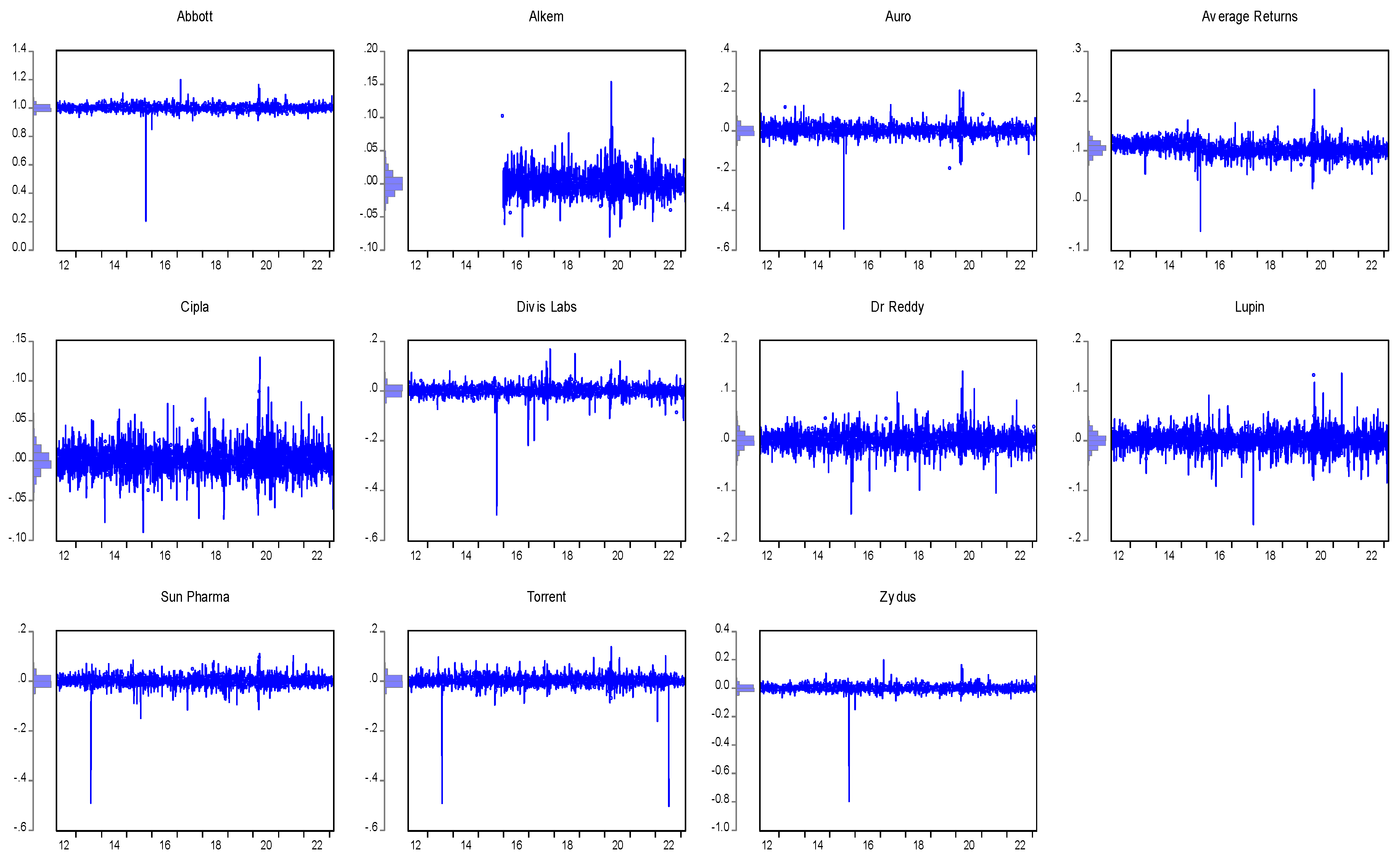
Figure 2 shows the volatility in daily returns of the top pharma markets in India during the specified period. The top 10 companies are considered part of the sample that represents the Indian pharma market.

Figure 2’s representations of return swing volatility plots aid in interpreting GARCH-M estimates. Features of distributions and assumptions of normalcy are assessed using the Histogram of Returns. When the returns are somewhat erratic, the series exhibits even greater volatility; when returns are relatively steady, there is relative quiet. The GARCH-M model effectively captures this regular feature of financial markets. Many shares have seen dramatic declines, possibly related to significant market shocks, news impact, or events influencing particular companies. Among the notable data, anomalies are sudden, and there are sharp declines in stock returns for Alkem, Sun Pharma, and Zydus. Some stocks—like Lupin, Cipla, and Dr. Reddy—seem less volatile in their return movements. Among those with more frequent and significant deviations than others are Torrent, Sun Pharma, and Alkem; others show more volatility.

Table 1. Descriptive statistics of daily returns [(V_.T. − V_T−1)/V_T−1].

	ABBOTT	ALKEM	AURO	CIPLA	DIVIS_LABS	DR_REDDY	LUPIN	SUN_PHARMA	TORRENT	ZYDUS
Mean	1.000	0.001	0.001	0.001	0.001	0.000	0.000	0.000	0.001	0.000
Median	1.000	0.000	0.000	−0.000	0.001	0.000	0.000	0.000	0.000	−0.000
Maximum	1.200	0.154	0.204	0.130	0.167	0.139	0.135	0.110	0.137	0.199
Minimum	0.204	−0.080	−0.492	−0.090	−0.497	−0.146	−0.168	−0.490	−0.503	−0.796
Std.Dev.	0.025	0.016	0.026	0.016	0.022	0.017	0.018	0.021	0.023	0.025
Skewness	−11.545	0.832	−2.122	0.570	−4.830	0.024	0.005	−4.862	−7.672	−11.545
Kurtosis	386.980	9.703	52.821	7.645	113.200	10.692	10.204	116.958	175.810	386.980
Jarque–Bera	1,666,552	3537.646	281,578.8	2576.835	1,378,229	6663.250	5846.336	1,473,261	3,389,870	16,665,527
Probability	0.000	0.000	0.000	0.000	0.000	0.000	0.000	0.000	0.000	0.000
Sum	2703.836	1.074	2.417	1.439	2.021	1.290	0.656	1.168	1.688	0.836
SumSq.Dev.	1.685	0.487	1.904	0.727	1.284	0.764	0.906	1.186	1.391	1.685
Observations	2703	2703	2703	2703	2703	2703	2703	2703	2703	2703

Source: author’s calculation.

contains descriptive statistics on the daily returns of the pharma sector. Based on the mean and median returns, ABBOTT has shown the maximum jump and gave the highest mean return in daily return with a value of 100.03%, while other stocks show almost nil median returns, implying sporadic imbalance. Also, ABBOTT has the maximum return from the entire dataset with a value of 119.94%. However, Zydus can be observed as recording a maximum loss of 79.57%. While Auro (0.0265), Abbott (0.00249), and Zydus (0.0249) are quite variable, Alkem, Cipla and Dr. Reddy are resolved to be more steady in terms returns as indicating least volatility due to lower standard deviation. The extreme values of Zydus (−0.7956) and Torrent (−0.5027) caused notable losses, stressing the likelihood of adverse outcomes. Most equities have negative skewness, which causes consistent and rather large falls. A high kurtosis (e.g., Abbott: 386.97) indicates notable price movements.

Table 2. Correlation matrix.

	Sun Pharma	Divis Labs	Dr Reddy	Cipla	Torrent	Zydus	Abbott	Alkem	Lupin	Auro	Average Returns
Sun Pharma	1
Divis Labs	0.231	1
Dr Reddy	0.343	0.300	1
Cipla	0.365	0.311	0.376	1
Torrent	0.170	0.194	0.196	0.213	1
Zydus	0.241	0.204	0.261	0.253	0.201	1
Abbott	0.241	0.204	0.261	0.253	0.201	0.9	1
Alkem	0.173	0.160	0.177	0.202	0.181	0.244	0.244	1
Lupin	0.381	0.282	0.389	0.438	0.231	0.294	0.294	0.183	1
Auro	0.311	0.274	0.326	0.351	0.194	0.259	0.259	0.199	0.351	1
Average Returns	0.530	0.486	0.538	0.552	0.440	0.651	0.651	0.283	0.588	0.585	1

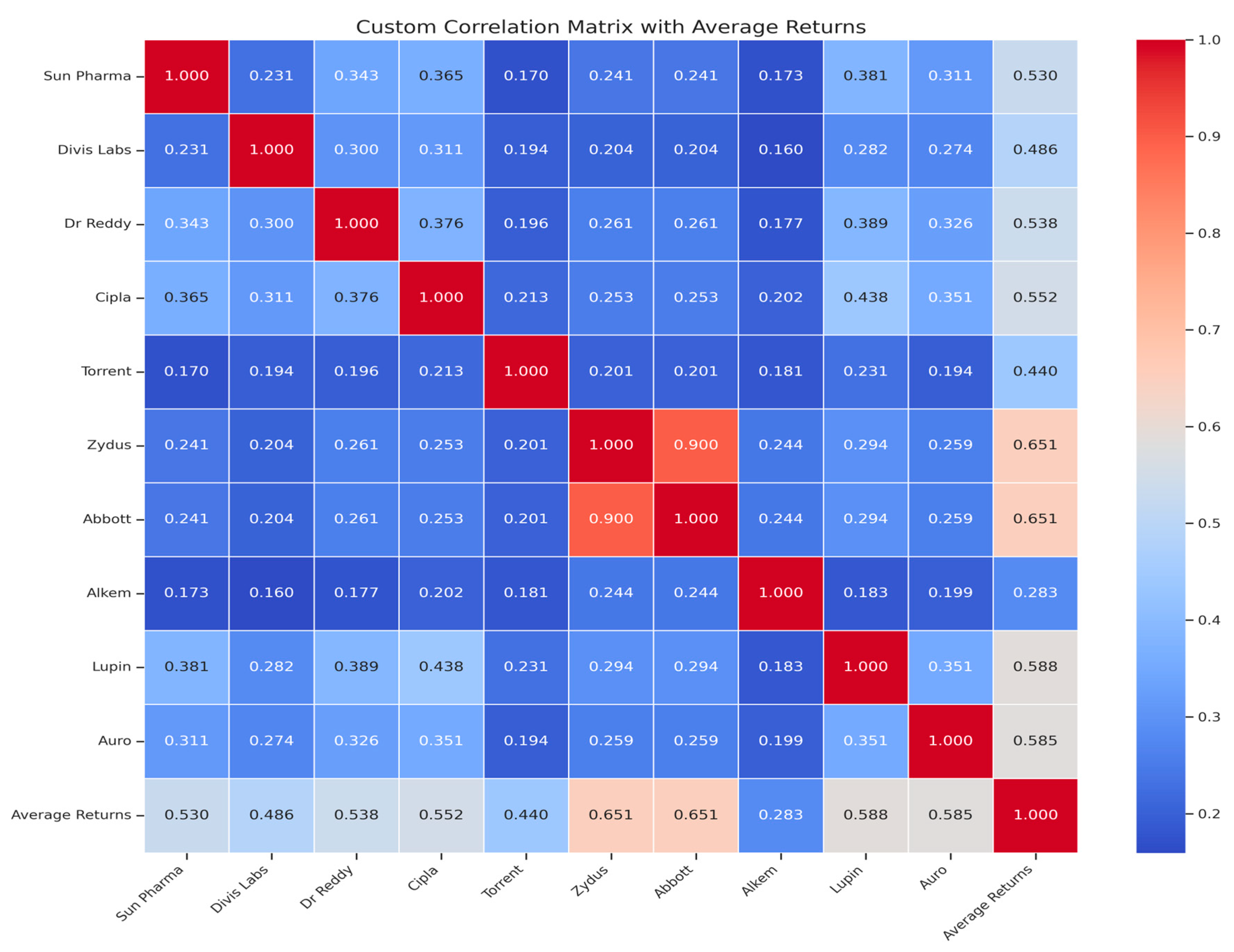
Source: author’s calculation.

and Figure 3 contain a correlation matrix of the daily returns of companies in the pharma sector in India. These projections of correlation with the industry provide useful insight to individual and institutional investors into which firms are growing in sync with other firms and which firms are envisioning a different direction in terms of returns. Moreover, to deepen the analysis, the correlation of the return of the sample with the average returns is also examined. From the correlation analysis, it can be interpreted that, apart from Torrent and Alkem, all other pharma returns are at a reasonable level of positive correlation.

Lupin and Dr. Reddy (0.389), Sun Pharma and Cipla (0.3655), Lupin and Cipla (0.4385), and Dr. Reddy and Cipla (0.3759) show notable co-movement, indicating they all influence the same market. Abbott and Zydus’s stock price movements are related with an astonishingly strong correlation of 0.9. Most of the correlations between pharmaceutical equities show modest links falling between 0.2 and 0.3, thus offers moderate diversification. Alkem and other firms have smaller correlations, which points to a different risk–return profile and such stock pairs tend to move more independently, offering better diversification. A lower stock correlation—say, Torrent at 0.2135—may lower the total risk of a portfolio. Notably, highly connected stocks like Abbott and Zydus provide no variety. Investors seeking high-risk, high-reward ideas could focus on stocks with a strong return correlation, including Lupin, Cipla, and Dr Reddy. Risk-averse investors would look for low-correlation pairs to help to lower volatility.

Table 3. ARMA modeling coefficient analysis.

Variable	Coefficient
	Overall	Pre-COVID-19	During COVID-19
C	0.000	0.000	0.000
AR(1)	0.072 *	0.067 *	0.075 *
MA(1)	−0.986 *	−0.984 *	−1
SIGMASQ	0.0001 *	0.0001 *	0.0001 *

Source: author’s presentation. * indicates statistically significant.

shows the coefficient analysis of the ARMA modeling. The model is based on two parameters: AR (autoregressive) and MA (moving average). Considering AR, it can be interpreted that, in the overall time frame, during and before the COVID-19 pandemic, the lag values significantly impact the given values. Moreover, considering the moving average, because of the COVID-19 lockdown, the impact of lagged error term became insignificant during the COVID-19 pandemic.

Table 4. ARMA modeling: regression statistics.

Variable	Coefficient
	Overall	Pre-COVID-19	During COVID-19
R-squared	0.000	0.000	0.000
Adjusted R-squared	0.456	0.456	0.460
S.E. of regression	0.011	0.011	0.012
Sum-squared resid.	0.349	0.245	0.102
Log-likelihood	8262.808	6068.994	2196.534
F-statistic	755.985	553.0052	208.147
Prob. (F-statistic)	0	0	0
Mean dependent var.	0.000	0.000	0.000
S.D. dependent var.	0.0154	0.015	0.016
Akaike info criterion	−6.113	−6.151	−6.015
Schwarz criterion	−6.104	−6.140	−5.990
Hannan–Quinn criteria	−6.111	−6.147	−6.005
Durbin–Watson stat.	2.003	2.000	2.001

Source: author’s presentation.

contains the regression statistics of the ARMA modeling. The value of the regression coefficients is 0.45, which signifies a low prediction rate of current values from the lag and error values. The values obtained in Table 3 and Table 4 are based on the ARMA Maximum Likelihood (OPG–BHHH) method, which includes a total of 2702 observations, out of which 1972 are from the pre-COVID-19-pandemic era and 729 are from the lockdown period. Considering the overall assessment of volatility in the Indian pharma sector, convergence was achieved after 30 iterations.

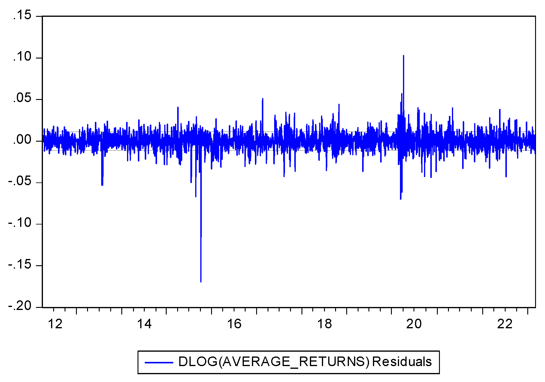
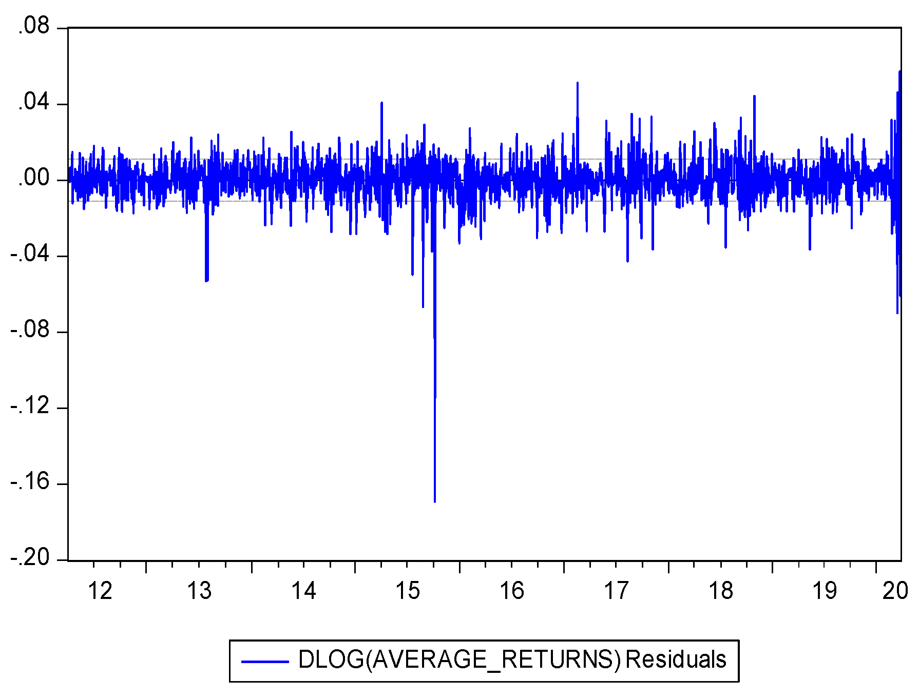
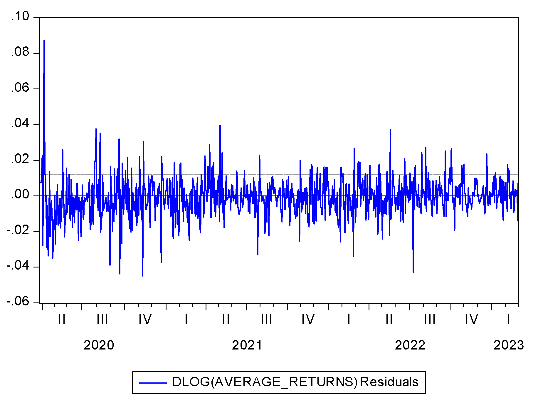
Figure 4, Figure 5 and Figure 6 contain residual graphs of overall returns, pre-COVID-19-pandemic and post-lockdown returns. These graphs provide a visual analysis of volatility clustering. The three residual graphs shown here show pharmaceutical company returns before, during, and after the COVID-19 pandemic. From a time-series model of stock returns, these graphs show the residuals, i.e., the errors. Usually referred to as white noise, the pattern-free, random residuals show that the model fits rather well.

Including pre- and post-COVID-19-pandemic years, the residual graph shows the overall return residuals. Given the near-negligible fluctuations, the model captures the trend in returns. Extreme spikes (outliers) could be indicators of market shocks brought on by broad economic events or pharmaceutical industry developments, including new drug approvals or legislative changes. Heteroskedasticity-changing variance across time may be used to demonstrate varying volatility.

Notwithstanding significant changes, the residual return graph from before the COVID-19 pandemic appears constant. Market outcomes were more predictable since there were less severe outliers before the outbreak. The minimal volatility of the pharmacy market at this time point implied regular market circumstances. Variations could come from mergers, acquisitions, and announcements about research and development.

Especially in the first stage, the residual graph shows higher volatility after the lockout. Some significant residual increases, which point to extreme market uncertainty, could be explained by investor responses to pandemic disruptions, vaccination campaigns, or legislative interventions. The post-COVID-19-pandemic distribution of residuals makes future stock returns less predictable. Significant differences expose slow market stabilization after the stopgap.

Table 5. Heteroskedasticity test: ARCH.

Particulars	Overall	Pre-COVID-19	During COVID-19
F-statistic	5.647	1.187	10.033
Obs*R-squared	11.260	2.375	19.606
Prob. F	0.004	0.305	0.000
Prob. Chi-squared (2)	0.004	0.305	0.000

Source: author’s calculation. * indicates statistically significant.

and

Table 6. Heteroskedasticity test: ARCH coefficient analysis.

Variable	Coefficient
	Overall	Pre-COVID-19	During COVID-19
C	0.000 *	0.000 *	0.000 *
RESID2(-1)	0.058 *	0.030	0.157 *
RESID2(-2)	0.025	0.017	0.029

Source: author’s calculation. * indicates statistically significant.

contain values based on the null hypothesis that no ARCH effect or volatility clustering exists. In Table 5, the F-statistic (5.6471) and prob. F (0.0036) exhibit significant heteroskedasticity; the variance in residuals is not constant for the overall period. Low p-values (<0.05) show that, as stock returns varied, external events or structural breaks influenced the pharmaceutical industry results. The ARCH effect exists, and we reject the null hypothesis.

The high p-values (0.3054, 0.3050) and F-statistic (1.1870) of the pre-COVID-19-pandemic period point to consistent stock returns in Table 5. The more constant residual pattern suggests that pre-pandemic market conditions were normal. Thus, the ARCH effect is not present.

The low p-value (0.0001) and F-statistic (10.0331) of the COVID-19-pandemic period show significant return heteroscedasticity, implying a high ARCH effect present, and it is validated that the volatility is time-dependent and related to a surge in risk and unpredictability. Supply chain disruptions, lockdown policies, vaccination approvals, and pandemic market reactions might cause extreme volatility and irregular shocks in the pharmaceutical industry.

Thus, we reject the null hypothesis for overall and post-COVID-19-pandemic return volatility. This means that, before the lockdown, because of the COVID-19 pandemic, there was no volatility clustering present in India’s pharma market; volatility clustering became so significant that the entire time frame had values exhibiting the ARCH effect.

The heteroskedasticity test is based on the lags of residuals. Present research considers two lags of residual 2, and the impact of the COVID-19 pandemic on heteroskedasticity is shown in Table 6. An insignificant second lag can be interpreted from the table in all three cases. However, considering the first lag, it can be observed that there was an insignificant impact on the residuals of the dataset before the COVID-19 pandemic. Though volatility does not seem to have a major influence on returns over the long term as per the overall period effect, pharma stock returns seem to be gaining speed on a sporadic basis. Despite shocks after the COVID-19 pandemic, pharmaceutical stock prices recovered fast; higher volatility led to lower returns. Market uncertainty during the COVID-19 pandemic upset the usual risk–return ratio, causing frequent price volatility and sudden corrections. Nevertheless, when the COVID-19 pandemic hit the Indian market, the impact on residuals became significant.

Table 7. Regression statistics: heteroskedasticity test, ARCH.

Particulars	Overall	Pre-COVID-19	During COVID-19
R-squared	0.004	0.001	0.027
Adjusted R-squared	0.003	0.000	0.024
S.E. of regression	0.001	0.001	0.000
Sum-squared resid.	0.001	0.001	0.000
Log-likelihood	16,004.410	11,511.930	4727.400
F-statistic	5.647	1.187	10.033
Prob. (F-statistic)	0.004	0.305	0.000
Mean dependent var.	0.000	0.000	0.000
S.D. dependent var.	0.001	0.001	0.000
Akaike info criterion	−11.853	−11.684	−12.997
Schwarz criterion	−11.846	−11.676	−12.978
Hannan–Quinn criter.	−11.850	−11.681	−12.990
Durbin–Watson stat.	2.001	2.002	2.003

Source: author’s calculation.

contains regression statistics from the heteroskedasticity test, calculated by least squares, taking RESID² as the dependent variable. The values of R² and adjusted R² in all three time frames are extremely low, depicting a poor prediction.

Table 8. GARCH-in-Mean: coefficient analysis.

Variable	Coefficient
	Overall	Pre-COVID-19	During COVID-19
GARCH	−0.095	−0.329 *	−0.045
C	0.000	0.000 *	0.000
AR(1)	0.091 *	0.120 *	0.052
MA(1)	−0.988 *	−0.998 *	−1.009 *

Source: author’s calculation. * indicates statistically significant.

demonstrates that there is no significant relationship between variance and returns regarding the overall assessment and post-lockdown period. However, the pre-COVID-19-pandemic era shows a significant link between variance and return and lockdown because the COVID-19 pandemic made it insignificant.

Table 9. GARCH-in-Mean: variable equation.

Variable	Coefficient
	Overall	Pre-COVID-19	During COVID-19
C	0.000 *	0.000 *	0.000 *
RESID(-1)2	0.104 *	0.078 *	0.127 *
GARCH(-1)	0.783 *	0.847 *	0.685 *
T-DIST. DOF	5.066	5.192 *	5.321 *

Source: author’s calculation. * indicates statistically significant.

shows the presence of a small but significant positive return for C (0.0000134) across the whole period, which shows the constant baseline return of pharmaceutical equities. The relatively strong positive coefficient RESID(-1) (0.104001)* indicates that historical return shocks affect current volatility. GARCH(-1) (0.783172) indicates persistent volatility; it maintains high values over extended periods. The pre-COVID-19-pandemic era showed a steady but lower baseline return (C = 0.00000832)* compared to the whole period. Based on RESID(-1)² (0.077904), which was substantial but lower than that during the COVID-19 pandemic, historical return shocks had a negligible effect on volatility. GARCH(-1) (0.847237)* indicates long-term high volatility or high volatility persistence. Compared to the whole period, the T-statistic (5.191616) grew a little and showed reduced fat tails and fewer severe returns. The rising demand for pharmaceutical equities suggests more significant baseline returns; therefore, C (0.0000244) surged during the COVID-19 pandemic. Previous shocks caused the market to respond faster and more intensely, as seen by the greatest RESID(-1)² (0.12749). GARCH(-1) (0.684643) shows reduced persistence and faster settlement than before the COVID-19 pandemic. The T-statistic (5.32183), which indicated less fat-tailed distribution and less severe price volatility, was the highest of all eras. The implication is that, though it decreased more quickly than before, COVID-19 pandemic market shocks brought fast volatility. The rising demand for pharmaceutical equities suggests more significant baseline returns; therefore, C (0.0000244) surged during the COVID-19 pandemic. Reflecting robust and fast market reactions to historical shocks, 0.12749 RESID(-1)² reflects the highest value of all time. Among all the periods, the T-statistic (5.32183) was the greatest, implying less fat-tailed distribution and fewer marked price fluctuations. GARCH (0.684643) shows faster settlement due to lower volatility compared to before the COVID-19 pandemic.

The GARCH-M model, which indicates Pharma stock volatility clustering, demonstrates that prior shocks cause future volatility and significant price movements. Before the COVID-19 pandemic, investors had time to adjust to market conditions since volatility was constant but less sensitive to transient shocks. Market behavior changed during the COVID-19 pandemic, and volatility became less persistent but more impactful and extreme. Though it passed faster than ever, the COVID-19 pandemic produced significant market instability.

5. Discussion and Implications

The inception of the COVID-19 pandemic has impacted every sphere of activity, industry, production, and stock market prices. Through the use of the MGARCH model, the current analysis indicated and concluded that, before the start of the COVID-19 pandemic, there was a substantial association between the risk taken by pharmaceutical businesses in India and the return on investment. However, after the COVID-19 pandemic struck and lockdowns were implemented, the correlation between risk and return was rendered meaningless. A study by Das et al. (2022) has documented that the COVID-19 pandemic has significantly lowered the stock market’s volatility, by analyzing the equity and bond indices with the help of the TGARCH method. It has been inferred by Karmakar (2007) that volatility is predictable, persistent, and clustered based on time. Volatility has not been correlated with risk and is asymmetrical to the previous function. It also shows a slow rate of increase in share prices. At the same time, an economic downturn, identified through an EGARCH analysis, was observed in the Nifty index of S&P for 14 years, ranging from 1990 to 2004. Stock return volatility has further been inferred by Yong et al. (2021) concerning the stock index data of Singapore and Malaysia before and during the COVID-19 pandemic, which showed persistent returns for both indices by employing the EGARCH, MGARCH, and PGARCH models. However, a negative relationship between return and volatility is established due to the incidence of leverage by employing the EGARCH model. According to Xing and Howe (2003), the bivariate GARCHM model is more reliable and provides useful predictions compared to the univariate GRACHM model, after having analyzed a positive relationship identified between U.K. stock market returns and world stock market return variance. Additionally, Hongsakulvasu and Liammukda (2020) recognize the significant positive relationship between return and risk in the foremost oil markets, including the Singapore Exchange, Brent, Dubai, and West Texas, during the COVID-19 pandemic, which also witnessed oil price conflicts (Sharma et al. 2023). The correlation between two less-correlated assets was measured by Yıldırım et al. (2022). The strengthened negative correlation between oil and gold and vice-versa with oil and silver has been demonstrated after the COVID-19 pandemic. The current study used the MGARCH model and inferred that, before the COVID-19 pandemic, there was a significant relationship between risk and return of the pharma sector in India. However, when the COVID-19 pandemic struck and lockdowns were implemented, the relationship between risk and return became insignificant.

Managerial Implications

The GARCH-M model highlights the increased volatility after the COVID-19 pandemic and shows that pharmaceutical stocks have a higher risk–return tradeoff. Investors might use these data to adjust their risk exposure. Optimizing entry and exit strategies and allocating assets dynamically based on market circumstances is possible through market timing and capturing time-varying volatility. Some stocks perform better than others during crises, according to correlation studies. By adding equities with lower volatility to investors’ portfolios and diversifying holdings, reducing exposure to extreme market fluctuations is possible. Briefly, investors could hedge risk by combining high-volatility stocks, like Auro and Zydus, with low-volatility stocks, such as Cipla and Dr Reddy, to balance risk and reward before the COVID-19 pandemic. During the COVID-19 pandemic, quick tactical adjustments were made involving high-frequency trading and adaptive hedging methods. Following the COVID-19 pandemic, risk models were updated to consider macroeconomic factors and policy changes were implemented as events unfolded. Better funding and capital allocation decisions by pharmaceutical companies can be made in uncertain scenarios with the model’s assistance in assessing volatility before and after a pandemic. Companies should build trustworthy alliances because rising volatility could affect decisions on M&A and long-term investment plans. For stabilizing stock prices, companies can win back the trust of their investors by implementing policies that reduce the frequency and severity of stock price fluctuations, such as more accurate profit forecasts and transparent financial reporting. Policymakers must monitor times of higher volatility since large swings are responsible for compromising market steadiness and introducing stabilizing strategies, such as circuit breakers, liquidity protections, and R&D funding in the light of a pandemic’s volatility, hence minimizing speculation during health emergencies and protect investors. Governments may incentivize research and development investments in pharmaceutical stocks that have demonstrated resilience to guarantee continuous healthcare improvements. Investors, pharmaceutical companies, and lawmakers can all benefit from the GARCH-M model’s comprehensive risk analysis, which covers periods before and after the COVID-19 pandemic. Stakeholders must understand volatility patterns to ensure better risk management, stable markets, and sustained sector growth in the post-pandemic era.

6. Conclusions

The BSE healthcare index performing excellently, with a compounded annual growth return of 12% during the last ten years compared to the Nifty pharma index (10.94%) and its other counterparts. Indian pharma companies are performing better than multinational pharma companies operating in India in terms of profitability and turnover due to the presence of an efficient in-house research and development center, which is the backbone of any pharma company (Nagarkar and Rao 2017). The growth factors contributing to the success of the Indian pharma sector are cost-effective manufacturing, a skilled workforce at low cost, large-scale production, and digital technology. Besides this, Indian pharma companies devote 2% to 10% of their income to research and development. However, significant obstacles along the way are insufficient pharma infrastructure, such as labs, machines, and clinics, and a high rate of inflation, resulting in increased production costs. Increased digitalization in the pharma industry also had to overcome resistance to change from employees and organizations used to practicing decade-old ways of conducting business; cooperation, integrity, and more transparency are needed for its greater acceptability.

It is apparent from this study that the pharma sector has huge growth potential and good investment opportunities, so the results drawn in the current article could be useful for estimating return volatility and investment decisions in the selected top ten pharma companies of India. However, this study has some limitations due to the inclusion of only the top ten Indian pharma companies instead of all Indian pharma companies.

Table 2 exhibits a correlation matrix where Sun Pharma and Cipla (0.3655), Lupin and Cipla (0.4385), and Dr. Reddy and Cipla (0.3759) show notable co-movement, indicating they all influence the same market. Abbott and Zydus’s stock price movements are related with an astonishingly strong correlation of 0.9. A lower stock correlation—say, Torrent and Cipla at 0.2135—may lower the total risk of a portfolio. Investors seeking high-risk, high-reward ideas could focus on stocks with a strong return correlation, including Lupin, Cipla, and Dr Reddy. Risk-averse investors would look for low-correlation pairs to help to lower volatility.

In Table 5, the F-statistic (5.6471) and prob. F (0.0036) exhibit significant heteroskedasticity; the variance in residuals is not constant for the overall period. The low p-values (<0.05) show that, as stock returns varied, outside events or structural breaks influenced the pharmaceutical industry results. Thus, a moderate ARCH effect exists, and we reject the null hypothesis; it indicates that volatility depends on past residuals.

Table 6 depicts that the COVID-19 pandemic brought about a spike in volatility; earlier shocks significantly influenced later price changes. Risk-adjusted models (like GARCH) are thus necessary for accurate forecasting in an environment of high market uncertainty. Mixed volatility patterns show that the market was stable before the COVID-19 pandemic. Hence, prior performance had little effect on the current one. The notable volatility clustering of pharmaceutical stock returns during the COVID-19 pandemic showed that exogenous shocks (such as the virus) continuously unsettled the market, which was susceptible to historical volatility. Conversely, moderate ARCH long-term impacts show volatility effects, which certainly exist as the COVID-19 pandemic phase drives them.

The findings suggest that the volatility rose after the COVID-19 pandemic, but this was more because of changes in government policies and vaccines than because of regular market forces. Pricing patterns can be dominated by stock interventions, liquidity constraints, and sentiments during a crisis period when volatility becomes irrelevant. However, the findings suggest that, especially before the COVID-19 pandemic, the high GARCH(-1) coefficients support Merton’s ICAPM, which maintains that past volatility shapes future returns. This sort of activity is compatible with the way financial markets usually operate. Though it lowered more rapidly, early market volatility during the COVID-19 pandemic was more pronounced. The idea that crisis-driven uncertainty generates short-lived but significant risk effects is supported by the higher impact of shocks (increasing RESID(-1)², lower GARCH(-1)). With a notable negative GARCH coefficient, the higher risk–return tradeoff points to volatility already being considered in returns before the COVID-19 pandemic. This matches asset pricing theories. Market inefficiencies caused this cooperation to stop during the COVID-19 pandemic, which is visible though the performance of many companies, like Sun Pharma, Alkem, and Zydus, which show apparent volatility increases over the course of the pandemic, implying a change in uncertainty and market shocks. Large harmful spikes suggest that, despite the increasing risk, the risk–return link would have momentarily collapsed since acute uncertainty and panic-driven selling created volatility without the corresponding rewards.

From the GARCH term in Table 8, it can be observed and interpreted that, before the COVID-19 pandemic, there was a significant relationship between risk and return of the pharma sector in India. However, when the COVID-19 pandemic struck and lockdowns were implemented, the relationship between risk and return became insignificant, implying volatility did not significantly impact returns.

The Indian pharma industry’s quick expansion demands continued investigation to stay ahead of the exceptionally high levels of innovation. However, the current findings and other investigators have allowed certain inferences to be made. Since this is the case, investment in the pharma industry may also be significantly impacted by policymakers’ reactions or supportive actions. The current study concentrates on using GARCH-M to analyze returns in India’s pharma sector, indicating that the data are stationary and have a specific distribution of error components through volatility analysis. However, non-linear volatility trends generated by machine learning-based methods or stochastic volatility models such as BEKK, spillover, E-GARCH, and BECH can be incorporated to explore other features. A more comprehensive perspective that might represent market-wide ramifications could be obtained by comparing the transmission of volatility to different industries and considering macroeconomic variables like inflation, interest rates, and currency exchange rates. By examining these interconnected external dynamics influencing volatility and risk within the pharma sector, we can better predict potential shocks and mitigate risks arising from systematic economic changes. Notwithstanding its limits, this evaluation may aid individual and corporate investors and inform future volatility irrelevance approaches for crisis situations.

7. Future Directions

Future study directions should focus on expanding the scope and methodology of pharmaceutical sector volatility analysis during crisis periods. Volatility effects resulting from crises can also be studied using GARCH-MIDAS models, and the implementation of behavioral finance theory can also be explored. Investigators could conduct cross-sectoral comparative analyses to determine if the observed risk–return patterns are unique to pharmaceuticals or reflect broader market trends. Longitudinal studies examining post-COVID-19-pandemic recovery periods would provide valuable insights into market normalization patterns. The integration of advanced modeling approaches, such as combining machine learning algorithms with traditional GARCH models and exploring quantum computing applications, could enhance prediction accuracy. Expanding the analysis to international markets would help identify regional variations in risk–return relationships and cross-border effects. Future studies should also examine the impact of healthcare policies, regulatory changes, and government interventions on market stability. The incorporation of market microstructure analysis, ESG factors, and alternative data sources like social media sentiment could provide deeper insights into volatility drivers. Additionally, developing specialized risk assessment tools and early warning systems for extreme market movements would benefit investors and policymakers. Research into behavioral finance aspects, including investor sentiment and herding behavior during health crises, would enhance our understanding of market dynamics. Studies on supply chain disruptions and their relationship with stock volatility, along with analysis of how R&D announcements and innovation impact stock performance during crises, would contribute valuable insights to the field. These expanded research directions would significantly advance our understanding of pharmaceutical sector market behavior during global health crises and improve risk management strategies for future events.