Abstract
In this article, we extend the application of cooperative game theory to the so-called low-risk puzzle. Specifically, we apply concepts that consider hierarchies on the assets in the allocation of portfolio risk. These hierarchies have not previously been considered in portfolio risk allocation using cooperative game theory. We demonstrate our idea through a simulation study. Our results show that considering hierarchies can contribute to solving the low-risk puzzle. Our findings may advance further developments in portfolio theory.
Keywords:
low-risk puzzle; portfolio risk; cooperative game theory; hierarchy; permission values; wH values JEL Classification:
C71; G10; G11
1. Introduction
This article builds on previous studies of the so-called low-risk puzzle (also called the low-risk anomaly) by incorporating concepts from cooperative game theory. These studies have used concepts such as the Shapley value to allocate portfolio risk to individual assets. The Shapley value is probably the best-known value-like solution concept in cooperative game theory (Roth 1988). An advantage is that it takes into account all contributions that an asset makes to the risks of all other asset groups. When applying the Shapley value, no other structures in the set of assets are taken into account. In reality, however, there are many structures or relationships between assets. One such structure is represented by hierarchies between assets. An example of a hierarchical structure between assets is the relationship between a firm’s equity and its debt capital (Modigliani and Miller 1958). Another example is the interdependence between different asset classes such as stocks, bonds and commodities over time (Bekaert and Harvey 1995). These interdependencies could be structured hierarchically. In this case, the portfolio optimization problem consists of finding the optimal diversification across a set of potentially interdependent assets in order to maximize return and minimize the risk (Muzy et al. 2010). In addition, the hierarchical risk parity is an advanced investment portfolio optimization framework developed by Lopez de Prado (2016). In this approach, assets are grouped into clusters based on their correlations, forming a hierarchical tree structure. Our paper applies the values of cooperative game theories that take into account these hierarchies among assets when allocating portfolio risk across assets.
In addition to the conventional approach of assessing an asset’s risk on an isolated basis—as evidenced by metrics such as asset variance—capital market theory offers several techniques for the distribution of portfolio risk across distinct assets. These include the activity-based method (Hamlen et al. 1977), the Beta method (Homburg and Scherpereel 2008), the machine learning-based dynamic capital asset pricing model (Wang and Chen 2023) and the incremental approach (Jorion 1985). Furthermore, a large body of scientific literature has emerged that applies the methods of cooperative game theory, particularly the Shapley value (Shapley 1953), the nucleolus (Schmeidler 1969) and the value—also known as the cost gap method (Tijs and Driessen 1986)—to this problem (Auer and Hiller 2019, 2021; Balog et al. 2017; Colini-Baldeschi et al. 2018; Mussard and Terraza 2008; Ortmann 2016, 2018; Shalit 2020, 2023; Simonian 2019; Terraza and Mussard 2007).
Nevertheless, even in the absence of a cooperative game-theoretic approach, empirical evidence from capital market theory indicates that the measurement of risk for an asset has remained a significant challenge. Contemporary theory suggests that assets with higher returns inevitably carry a corresponding level of risk (Lintner 1965; Markowitz 1952; Mossin 1966; Rubinstein 2002; Sharpe 1964). Empirically, an opposing phenomenon has been observed, which is referred to as the ‘low-risk puzzle’. Moreover, the existence of this phenomenon remains consistent across different classical risk measures (Auer and Schuhmacher 2021; Baker et al. 2011; Blitz et al. 2014; Dutt and Humphery-Jenner 2013; Frazzini and Pedersen 2014). The empirical evidence indicates that assets with low risk (volatility) consistently generate higher returns, a phenomenon that remains consistent across global large-cap assets, as well as the U.S., European and Japanese markets. Moreover, the low-risk puzzle cannot be attributed to other factors, such as the book-to-market ratio or free float market value. This puzzle demonstrates resilience when evaluated across different periods of volatility measurement (Blitz and van Vliet 2007). The analysis by Schneider et al. (2020) indicates that the low-risk puzzle in the capital asset pricing model and in traditional factor models exist when investors require compensation for coskewness risk. A recent literature review is provided by Traut (2023). One potential explanation for this empirical phenomenon is the inherent challenge of allocating portfolio risk to individual assets (Baker et al. 2011). Auer and Hiller (2019; 2021) show, in simulation studies, that using the Shapley value instead of classical risk measures has the potential to solve the low-risk puzzle.
In addition to considering all marginal contributions, cooperative game theory provides a framework for the incorporation of a hierarchy between assets. In Gilles et al. (1992), van den Brink and Gilles (1996) and van den Brink (1997), values for games with a hierarchical structure (H values) were introduced. In H values, single-dominance relationships, i.e., the influence of a predecessor on direct successors, are equally strong. These values assume that a player has to obtain permission from all their superiors to generate a certain amount of worth. Without all superior players, a player could not be productive. In other words, the superiors of a player have veto power against the player. However, it is a plausible assumption that the relationships between players may have different strengths. Using this idea to improve the modeling of hierarchies, Casajus et al. (2009) introduced a weighted hierarchy value based on the Shapley value—the value. This approach uses a weighted directed graph to model hierarchies. Two elements form the basis of the value. First, all players cooperate symmetrically to produce the output. In this step, the output is distributed to the players according to the Shapley value (Shapley 1953). In a second step, the weighted hierarchy redistributes a certain fraction of these payoffs. The weighted hierarchy has only allocational effects.1 In Hiller (2014), the value has been generalized to games with a graph/network. One value for these games is the Myerson value, My (Myerson 1977). Hence, the value is one generalized wH value. In addition to games with hierarchical structures with directed graphs, there are analogous structures in cooperative game theory. These include undirected graphs/networks (Borm et al. 1992; Gómez et al. 2003; Herings et al. 2008; Myerson 1977; Navarro 2020), which were analyzed in Hiller (2023) and Hiller (2025) with regard to their contribution to solving the low-risk puzzle. In these games, the players are connected by a graph, but there is no superior–subordinate relationship between them. The undirected networks could be interpreted as communication channels. In addition, undirected graphs could model similarities between assets, e.g., branches, company size or the regional origin of an asset. Suppose that there are three assets: an American car manufacturer, an American technology company and a European technology company. The first and last assets have nothing in common, while the second asset is somewhere in between the other two and can ‘dock’ with both (Alvarez-Mozos et al. 2013). In van den Brink (2012), the distinction between hierarchies and undirected graphs/networks is explained in more detail and, in addition, with respect to economic applications. van den Brink et al. (2017) establish the formal connection between undirected graphs/networks and hierarchies. In games with level structures (Kalai and Samet 1987), players are divided into different levels, but there is no concrete assignment of a player from a lower level to a player in a higher level. The German stock market, for example, offers the DAX, MDAX and SDAX, which are different levels in terms of the market capitalization of companies.
As mentioned, games with a hierarchical structure are the starting point for our article. By simulation, we seek to analyze whether the technical inclusion of hierarchies on the set of assets can increase the number of corrections of the rankings between the assets—hence solving the low-risk puzzle. Concretely, we apply the H value, the value and the value. For our analysis, we conduct a simulation study based on the ideas of Auer and Hiller (2019, 2021). We consider an investor who is interested in combining individual assets into a portfolio and assess the riskiness of each asset based on payoffs according to the weights of assets. Our setup is designed such that the low-risk puzzle lies in the variances of the individual assets. We then generate the covariance matrix of the assets repeatedly at random. We consider three schemes for the asset shares in a portfolio. Based on these data, we calculate the asset risks and the percentage of cases in which they lead to asset rankings that differ from the individual asset variances. We also calculate Shapley risk distributions as a benchmark and determine whether there are more corrections when hierarchical relationships between assets are taken into account.
2. Cooperative Game Theory
2.1. Games
A transferable utility (TU) game in cooperative game theory is denoted by , where is the non-empty and finite set of players. The number of players in N is n or The coalitional function v assigns every subset a certain worth -the risk of a portfolio of K-i.e., where denotes the power set of N.
A value is an operator that assigns (unique) payoff vectors to all games , i.e., uniquely determines a payoff for every player in every TU game. One value is the Shapley value. In order to calculate the players’ payoffs, rank orders on N are used. They are written as , where is the first player in the order, the second player, etc. The set of these orders is ; rank orders exist. The set of players before i in rank order and player i is For we have (Shapley 1953)
2.2. Games
As in Gilles et al. (1992), van den Brink and Gilles (1996), van den Brink (1997), Casajus et al. (2009) and van den Brink and Dietz (2014), for example, a permission structure is a mapping To each player, we assign the players who are direct successors of S can be interpreted as a directed graph (Bollobás 2002). denotes the direct successors of with The players in are the direct predecessors of i;
For the hierarchy between assets, we assume a tree structure. Within this structure, a path T in N from i to j is a sequence with , and ∀. A path can be interpreted as a chain of commands or chain of reporting between i and j, whereby i is a predecessor of j. The set of successors of i is . Analogously, we denote the set of i’s predecessors by . A tree structure formally satisfies two conditions:
- there is one player , such that and , and
- for every player , we have .
A hierarchical game is a tuple For these games, a value is an operator Gilles et al. (1992), van den Brink and Gilles (1996) and van den Brink (1996) introduced two values —the conjunctive approach value and the disjunctive approach value. Both values coincide if the hierarchy has a tree structure. To calculate a player’s payoff, for each coalition , the feasible set has to be determined: The restricted coalitional function is given by
Based on this function, the conjunctive approach value and the disjunctive approach value calculate player’s i payoff by
2.3. Games
One disadvantage of the concepts for games is that the hierarchical relationship is fixed. Besides the hierarchy S, weighted relationships between the players can be considered. The vector assigns every player i a weight with If a vector maps all players with the same weight , except i.e., for all we denote the vector by . A weighted hierarchical game is a tuple A value for these games is an operator The value is one value for . All players with respectively, and all players in the path , receive a fraction of g’s Shapley payoff. For , the fraction of s payoff is (Casajus et al. 2009)
From this, we have, for the payoff of player ,
To honor players who coordinate other players, the wH value based on the Myerson value (Myerson 1977) has been axiomatized (Hiller 2014). Some further preliminaries are necessary to introduce this value. First, a graph L on the set of players is considered. The set of possible pairwise links between players is whereat and respectively (or and ), is the direct link between players i and j. A cooperation structure CO on N is a graph with A CO game is characterized by . From hierarchy we construct : ∀; thus, the CO game results. The graph partitions N into components This partition is called Each player is in one component; denotes the component of i. Two players i and j with are connected. The restricted coalitional function is given by
The worth of a coalition K is the sum of the worth of its components. In the case , we have A CO value is an operator that assigns (unique) payoff vectors to all CO games. One CO value is the Myerson value (Myerson 1977). According to this value, player s payoff is2
With these preliminaries, is (Hiller 2014, 2021)
For a literature review regarding values in games with hierarchies, see van den Brink (2017).
3. Simulation
3.1. General Setting
In our application, we determine the coalition function v by
whereby are asset weights; are correlations between two assets i and j; and are standard deviations.
Since our study is similar to those by Auer and Hiller (2019, 2021), we adopt some of their simulation settings. We analyze a three-asset scenario, We assume mean returns and variances Therefore, the low-risk puzzle emerges, given that the asset with the lowest risk/variance (asset 1) achieves the highest return. Further, we have a covariance matrix of asset returns. For asset shares , we have In this study, we analyze three asset allocation schemes within a portfolio. In the first weighting scheme, the investor is assumed to be a minimum-variance investor with respect to . Thus, the asset weights are determined in such a way that is minimized. The second weighting scheme has random shares assuming a uniform distribution of asset shares between 0 and The third scheme is a naive one with
Furthermore, we implement an additional technical configuration of the simulation proposed by Auer and Hiller (2019). The covariance matrix and the asset shares in the second weight scheme are simulated 100,000 times; the standard deviations of assets range from 0 to 10 and asset correlations range from to 3
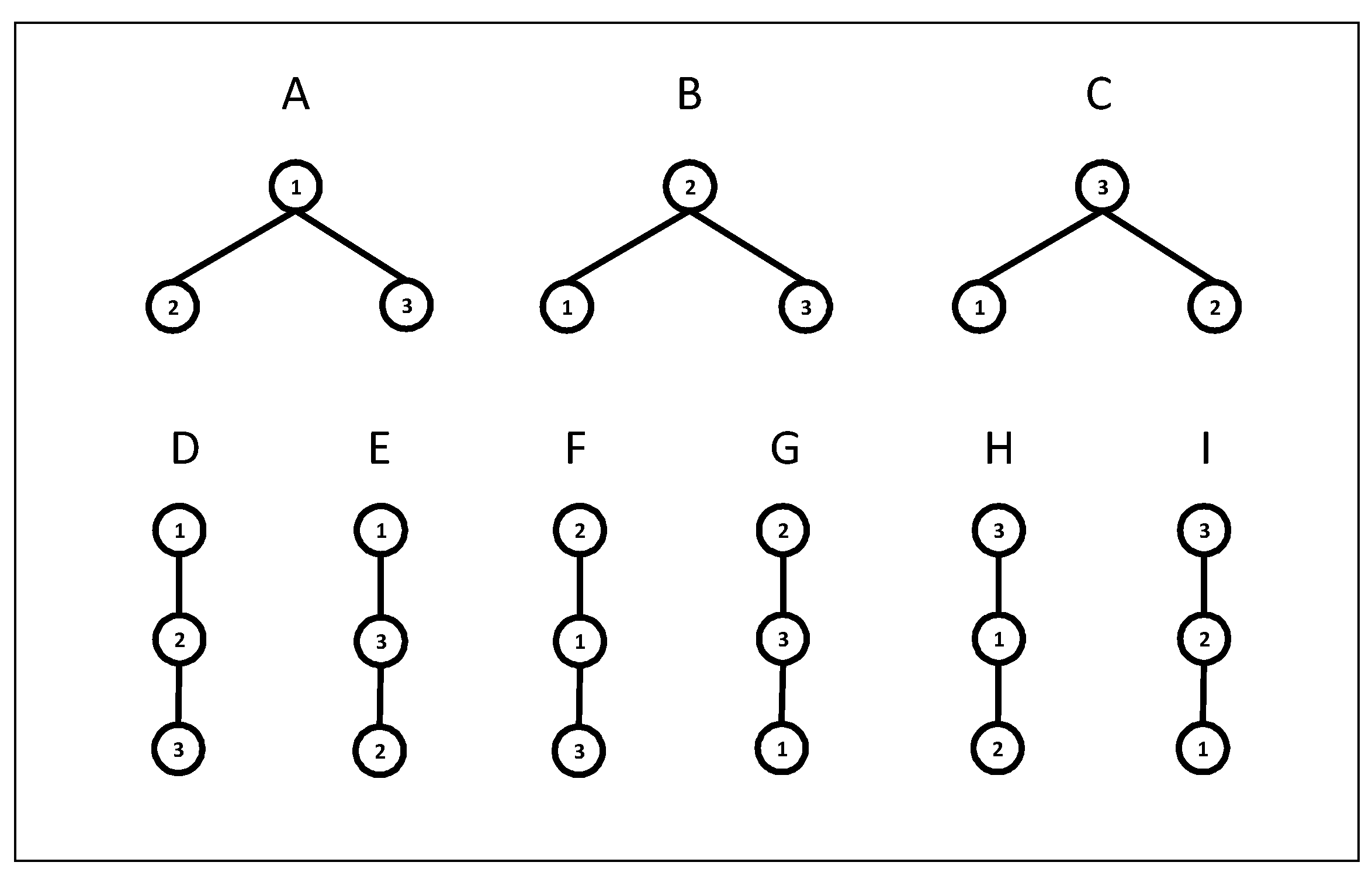
We consider the hierarchies shown in Figure 1. In each of the hierarchies A to C, one asset is at the top of the hierarchy and the other two assets are direct successors of this asset. In hierarchies D to I, the asset at the top of the hierarchy is directly followed by only one asset. The third asset is the direct successor to this asset. In addition, we assume four weight vectors with respect to the value and the value- -and random weights assuming a uniform distribution of between 0 and This broad approach, with all possible hierarchical structures on the set of three assets and a variety of weight vectors, allows for a detailed analysis of how hierarchies affect the correction of the low-risk puzzle.
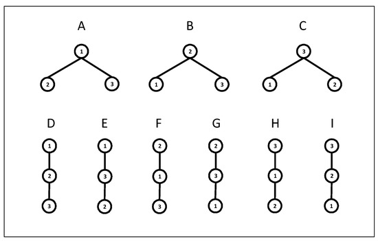
Figure 1.
Hierarchies.
3.2. Analytical Framework
Our results reflect the proportions of cases in which
- a rank correction between assets 1 and 2;
- any partial correction (two assets change ranks); or
- full correction
occurs. In addition, we compute the so-called risk–return relationship. We apply the least-squares method to a linear equation linking the mean return vector (with arbitrary values of [3 2 1] for the assets) to the risk allocation vector (computed by the weighted values). Very similarly, Auer and Hiller (2021) use this method to analyze the best remedy for the low-risk anomaly on the basis of cooperative game theory values. If the slope of the regression line is positive, the low-risk puzzle is solved for the average. In our analysis, the results of the Shapley value are used as benchmarks (Table 1). We analyze in detail our results for asset weights that minimize

Table 1.
Results for the Shapley value.
3.3. Results for the H Value
The first results analyzed are those for the H value (Table 2). With *, we mark results that are above the results of the Shapley value. Hierarchies C, D, E and I correct better between assets 1 and 2 with respect to Shapley. In hierarchies D and E, asset 1 is on top in the hierarchy and asset 2 is on a lower level. In hierarchies C and both assets are not at the top position, and, for both assets, the chances of making marginal contributions are greatly reduced. If any directional correction is considered, all hierarchies except H perform better compared to Shapley. With respect to full corrections, only hierarchies D and E outperform Shapley. Regarding the proportion of positive risk–return relations, B, E and G provide better results than Shapley. Considering all four dimensions, hierarchies A, D and E improve the results in terms of solving the low-risk puzzle in all dimensions compared to Shapley.
Table 2.
Results for the H value, minimum-variance asset share.
3.4. Results for the Value
The next step is to look at the results for the value (Table 3). In terms of corrections between asset 1 and asset 2, hierarchies and I outperform the Shapley value with all weight schemes. For hierarchies H and I and all weights , more directional corrections occur with respect to Shapley. Considering full corrections, hierarchies E and I outperform Shapley. In the case of positive risk–return relationships, E and F yield higher proportions for all weight schemes. When all four dimensions are considered, hierarchies A and E perform better then Shapley. With respect to the weights for hierarchies D and E, a positive influence can be seen across all four dimensions. For the other hierarchies, a clear statement cannot be made. In no hierarchy do the weights have an exclusively negative influence. Table 4 compiles our results with respect to weights
Table 3.
Results for the wH Shapley value, minimum-variance asset share.
Table 4.
Influence of , wH Shapley value, minimum-variance asset share.
3.5. Results for the Value
Finally, we analyze our results for the value (Table 5). Again, we start with corrections between asset 1 and asset 2. For hierarchies D, E and I and all weights , more corrections occur compared to Shapley. Considering any directional correction, C, D, E, G and I and all weight schemes outperform the results for Shapley. If we consider full corrections, the hierarchies E and G obtain a higher number of corrections with respect to Shapley. Regarding all four dimensions, only hierarchy E performs better than Shapley. With respect to in hierarchies A, H and I, there is no negative influence for all four dimensions. For hierarchy C, we obtain no positive influence. In Table 6, the results with respect to weights are presented.
Table 5.
Results for the wH Myerson value, minimum-variance asset share.
Table 6.
Influence of , wH Myerson value, minimum-variance asset share.
3.6. Comparison of the Results
When comparing the values, we start by comparing and . Overall, the value leads to fewer improvements when directional corrections, full corrections and the proportion of positive risk–return relationships are considered. Only in a few cases, such as hierarchy G and when full corrections and the proportion of positive risk–return relationships are taken into account, does the value produce better results than the wH value.
If we compare the H value with the two wH values, it is noticeable that the H concept leads to more extreme results/proportions of corrections. Overall, the H value can lead to improvements in all four dimensions with three hierarchies. This is a result that does not exist at such a high level for the wH concepts. Thus, if the real-world hierarchical relationship between assets is very clear, the H concept can solve the entire low-risk puzzle. However, because of their weighting, the two wH concepts offer the possibility of mapping the dominance relationships between the assets in a more granular way, which may also better reflect the realities of the asset market. In Table 7, Table 8 and Table 9, we show the number of corrections/number of proportions with positive risk–return relationships above the results of the Shapley value for three hierarchy categories. The first category consists of hierarchies E and In these hierarchies, asset 1 is a direct/indirect predecessor of asset 2. The second category contains hierarchy In this hierarchy, neither asset 1 is a predecessor of asset 2 nor vice versa. Finally, the last category consists of hierarchies where asset 2 is a direct/indirect predecessor of asset 1.
Table 7.
Number of results above the results of the Shapley value for three hierarchy categories, H value, minimum-variance asset share.
Table 8.
Number of results above the results of the Shapley value for three hierarchy categories, wH Shapley value, minimum-variance asset share.
Table 9.
Number of results above the results of the Shapley value for three hierarchy categories, wH Myerson value, minimum-variance asset share.
Our results for the random asset shares and the naive weight scheme can be found in Appendix A. They do not differ from the results for asset weights that minimize .
4. Research Outlook
In our paper, the application of cooperative game theory to the problem of allocating portfolio risk to assets in portfolios has been extended. The results obtained show that the consideration of hierarchies may contribute to solving the low-risk puzzle.
We leave open the question of which hierarchical structure and which value for hierarchical games best solves the low-risk puzzle. The low-risk puzzle is an empirical problem. Therefore, empirical studies are the only means by which it is possible to determine the extent to which the presented approach could solve the low-risk puzzle. In addition to empirical analyses of which hierarchical values and which hierarchical structures make the greatest contribution to solving the low-risk puzzle, empirical studies could, for example, determine the optimal calibration/translation of the hierarchical strength of the relationship between assets in the approach and the approach. The ability to consider hierarchies between assets is just one building block that can help in solving the low-risk puzzle through cooperative game theory. In cooperative game theory alone, there are many other ways to model structures on the set of assets, such as coalition structures (Aumann and Dreze 1974; Casajus 2009; Owen 1977), asset weights (Béal et al. 2018; Haeringer 2006; Kalai and Samet 1987) and weighted level structures (Besner 2019, 2022). At best, some implications for the theoretical development of capital market models can be drawn from studies applying cooperative game theory, especially hierarchical games (Simonian 2019).
With respect to the methods of cooperative game theory, there are many approaches to modeling hierarchical structures. With regard to hierarchies, it is possible to dispense with the assumption of a tree structure. In this case, the conjunctive approach value and the disjunctive approach value generate different payoffs. Furthermore, as mentioned in the Introduction, undirected graphs/networks and level structures are similar approaches. van den Brink (2010) provides an approach where the Banzhaf concept (Banzhaf 1965) is the basis for the H value. The generalization of permission values using antimatroids is described by Algaba et al. (2003). Other concepts for the determination of player payoffs in hierarchical games have been introduced by del Pozo et al. (2011), Khmelnitskaya et al. (2016), Alvarez-Mozos et al. (2017), Algaba et al. (2018) and Algaba and van den Brink (2019). In addition, games with trees (Bilbao et al. 2006; Béal et al. 2010, 2022; Hamiache 1999, 2004; Herings et al. 2008; Kang et al. 2022; Navarro 2020) and digraphs (Borm and van Den Brink 2002) are structures that are similar to hierarchies.
Funding
Supported by the Open Access Publishing Fund of Leipzig University.
Data Availability Statement
The datasets generated and analyzed during the current study are available from the corresponding author upon request.
Conflicts of Interest
The author declares no conflicts of interest.
Appendix A
In addition to the results in our main text, we present results for two other weight schemes for the allocation of assets within a portfolio. The first scheme is a naive one, in which all assets are allocated an equal share; The second weighting scheme has random shares assuming a uniform distribution of asset shares between 0 and We have the following:
- Benchmark results for the Shapley value (Table A1);
- Results for H and equal asset shares (Table A2);
- Results for H and random asset shares (Table A3);
- Results for and equal asset shares (Table A4);
- Results for and random asset shares (Table A5);
- Results for and equal asset shares (Table A6);
- Results for and random asset shares (Table A7).
Table A1.
Shapley value for different weight schemes.
Table A1.
Shapley value for different weight schemes.
| Asset Share | Correction | Directional | Full | Proportion Pos. |
|---|---|---|---|---|
| 1 and 2 | Correction | Correction | Risk–Return Rel. | |
| equal | 0.1260 | 0.1789 | 0.0024 | 0.0109 |
| random | 0.1652 | 0.2303 | 0.0018 | 0.0099 |
| risk min. | 0.0961 | 0.1414 | 0.0024 | 0.0134 |
Table A2.
Results for the H value, equal asset share.
Table A2.
Results for the H value, equal asset share.
| Hierarchy | Correction | Directional | Full | Proportion Pos. |
|---|---|---|---|---|
| 1 and 2 | Correction | Correction | Risk–Return Rel. | |
| A | 1.0000 * | 1.0000 * | 0.1776 * | 1.0000 * |
| B | 0 | 1.0000 * | 0 | 0.1782 * |
| C | 0.3888 * | 0.3888 * | 0 | 0 |
| D | 1.0000 * | 1.0000 * | 0.6069 * | 1.0000 * |
| E | 1.0000 * | 1.0000 * | 0.1923 * | 1.0000 * |
| F | 0 | 1.0000 * | 0 | 0 |
| G | 0 | 1.0000 * | 0 | 0.5922 * |
| H | 0 | 0 | 0 | 0 |
| I | 1.0000 * | 1.0000 * | 0 | 0 |
* Results above the results of the Shapley value.
Table A3.
Results for the H value, random asset share.
Table A3.
Results for the H value, random asset share.
| Hierarchy | Correction | Directional | Full | Proportion Pos. |
|---|---|---|---|---|
| 1 and 2 | Correction | Correction | Risk–Return Rel. | |
| A | 1.0000 * | 1.0000 * | 0.2520 * | 1.0000 * |
| B | 0 | 1.0000 * | 0 | 0.1740 * |
| C | 0.3588 * | 0.3588 * | 0 | 0 |
| D | 1.0000 * | 1.0000 * | 0.6149 * | 1.0000 * |
| E | 1.0000 * | 1.0000 * | 0.2183 * | 1.0000 * |
| F | 0 | 1.0000 * | 0 | 0 |
| G | 0 | 1.0000 * | 0 | 0.5588 * |
| H | 0 | 0 | 0 | 0 |
| I | 1.0000 * | 1.0000 * | 0 | 0 |
* Results above the results of the Shapley value.
Table A4.
Results for the wH Shapley value, equal asset share.
Table A4.
Results for the wH Shapley value, equal asset share.
| Hierarchy | Weight | Correction | Directional | Full | Proportion Pos. |
|---|---|---|---|---|---|
| Vector | 1 and 2 | Correction | Correction | Risk–Return Rel. | |
| A | 0.25 | 0.2351 * | 0.2855 * | 0.0050 * | 0.0230 * |
| 0.50 | 0.4697 * | 0.5100 * | 0.0151 * | 0.0745 * | |
| 0.75 | 0.8738 * | 0.8855 * | 0.0437 * | 0.4364 * | |
| rand. | 0.5312 * | 0.5638 * | 0.0227 * | 0.2576 * | |
| B | 0.25 | 0.0601 | 0.1933 * | 0.0024 | 0.0109 |
| 0.50 | 0.0195 | 0.3280 * | 0.0006 | 0.0109 | |
| 0.75 | 0.0143 | 0.6474 * | 0.0001 | 0.0109 | |
| rand. | 0.0412 | 0.4405 * | 0.0012 | 0.0109 | |
| C | 0.25 | 0.1260 | 0.1499 | 0.0010 | 0.0051 |
| 0.50 | 0.1260 | 0.1371 | 0.0005 | 0.0025 | |
| 0.75 | 0.1260 | 0.1372 | 0.0006 | 0.0046 | |
| rand. | 0.1260 | 0.1464 | 0.0010 | 0.0064 | |
| D | 0.25 | 0.0385 | 0.1528 | 0.0053 * | 0.0180 * |
| 0.50 | 0.0531 | 0.2536 * | 0.0175 * | 0.0441 * | |
| 0.75 | 0.2169 * | 0.4575 * | 0.1129 * | 0.2224 * | |
| rand. | 0.2167 * | 0.3572 * | 0.1010 * | 0.1955 * | |
| E | 0.25 | 0.2796 * | 0.3065 * | 0.0029 * | 0.0179 * |
| 0.50 | 0.4807 * | 0.4928 * | 0.0040 * | 0.0531 * | |
| 0.75 | 0.8410 * | 0.8440 * | 0.0057 * | 0.3689 * | |
| rand. | 0.5371 * | 0.5538 * | 0.0041 * | 0.2495 * | |
| F | 0.25 | 0.3898 * | 0.4618 * | 0.0025 * | 0.0139 * |
| 0.50 | 0.4729 * | 0.6314 * | 0.0020 | 0.0192 * | |
| 0.75 | 0.3601 * | 0.7947 * | 0.0002 | 0.0295 * | |
| rand. | 0.3333 * | 0.6246 * | 0.0016 | 0.0228 * | |
| G | 0.25 | 0.0444 | 0.3027 * | 0.0015 | 0.0087 |
| 0.50 | 0.0150 | 0.5414 * | 0.0007 | 0.0066 | |
| 0.75 | 0.0073 | 0.8687 * | 0.0002 | 0.0052 | |
| rand | 0.0321 | 0.5752 * | 0.0007 | 0.0070 | |
| H | 0.25 | 0.0759 | 0.1206 | 0.0016 | 0.0077 |
| 0.50 | 0.0575 | 0.0831 | 0.0010 | 0.0048 | |
| 0.75 | 0.0517 | 0.0674 | 0.0005 | 0.0052 | |
| rand. | 0.0668 | 0.0978 | 0.0011 | 0.0079 | |
| I | 0.25 | 0.2056 * | 0.2185 * | 0.0015 | 0.0066 |
| 0.50 | 0.2896 * | 0.2938 * | 0.0007 | 0.0030 | |
| 0.75 | 0.3783 * | 0.3806 * | 0.0011 | 0.0029 | |
| rand. | 0.2927 * | 0.3034 * | 0.0021 | 0.0061 |
* Results above the results of the Shapley value.
Table A5.
Results for the wH Shapley value, random asset share.
Table A5.
Results for the wH Shapley value, random asset share.
| Hierarchy | Weight | Correction | Directional | Full | Proportion Pos. |
|---|---|---|---|---|---|
| Vector | 1 and 2 | Correction | Correction | Risk–Return Rel. | |
| A | 0.25 | 0.2803 * | 0.3421 * | 0.0051 * | 0.0269 * |
| 0.50 | 0.5139 * | 0.5608 * | 0.0200 * | 0.1257 * | |
| 0.75 | 0.8307 * | 0.8451 * | 0.0525 * | 0.5355 * | |
| rand. | 0.5514 * | 0.5906 * | 0.0277 * | 0.2944 * | |
| B | 0.25 | 0.0983 | 0.2517 * | 0.0022 * | 0.0099 |
| 0.50 | 0.0447 | 0.4048 * | 0.0011 | 0.0099 | |
| 0.75 | 0.0164 | 0.7263 * | 0.0004 | 0.0099 | |
| rand. | 0.0604 | 0.4960 * | 0.0010 | 0.0099 | |
| C | 0.25 | 0.1652 | 0.1876 | 0.0006 | 0.0043 |
| 0.50 | 0.1652 | 0.1712 | 0.0003 | 0.0018 | |
| 0.75 | 0.1652 | 0.1698 | 0.0003 | 0.0017 | |
| rand. | 0.1652 | 0.1816 | 0.0006 | 0.0040 | |
| D | 0.25 | 0.0712 | 0.1958 | 0.0054 * | 0.0192 * |
| 0.50 | 0.0892 | 0.2975 * | 0.0266 * | 0.0656 * | |
| 0.75 | 0.3810 * | 0.5891 * | 0.1781 * | 0.3472 * | |
| rand. | 0.2718 * | 0.4174 * | 0.1207 * | 0.2277 * | |
| E | 0.25 | 0.2999 * | 0.3278 * | 0.0023 * | 0.0197 * |
| 0.50 | 0.5092 * | 0.5171 * | 0.0034 * | 0.0892 * | |
| 0.75 | 0.8066 * | 0.8082 * | 0.0031 * | 0.5189 * | |
| rand. | 0.5507 * | 0.5674 * | 0.0025 * | 0.2833 * | |
| F | 0.25 | 0.3523 * | 0.4446 * | 0.0028 * | 0.0139 * |
| 0.50 | 0.4130 * | 0.6081 * | 0.0019 * | 0.0213 * | |
| 0.75 | 0.2787 * | 0.7895 * | 0.0007 | 0.0378 * | |
| rand. | 0.2914 * | 0.6176 * | 0.0017 | 0.0287 * | |
| G | 0.25 | 0.0849 | 0.3595 * | 0.0010 | 0.0074 |
| 0.50 | 0.0347 | 0.6212 * | 0.0006 | 0.0051 | |
| 0.75 | 0.0108 | 0.8911 * | 0.0001 | 0.0035 | |
| rand | 0.0523 | 0.6213 * | 0.0006 | 0.0055 | |
| H | 0.25 | 0.1388 | 0.1909 | 0.0011 | 0.0058 |
| 0.50 | 0.1173 | 0.1431 | 0.0006 | 0.0025 | |
| 0.75 | 0.1006 | 0.1109 | 0.0002 | 0.0020 | |
| rand. | 0.1199 | 0.1510 | 0.0007 | 0.0047 | |
| I | 0.25 | 0.2054 * | 0.2143 | 0.0012 | 0.0059 |
| 0.50 | 0.2578 * | 0.2596 * | 0.0007 | 0.0027 | |
| 0.75 | 0.3258 * | 0.3265 * | 0.0006 | 0.0016 | |
| rand. | 0.2684 * | 0.2775 * | 0.0012 | 0.0044 |
* Results above the results of the Shapley value.
Table A6.
Results for the wH Myerson value, equal asset share.
Table A6.
Results for the wH Myerson value, equal asset share.
| Hierarchy | Weight | Correction | Directional | Full | Proportion Pos. |
|---|---|---|---|---|---|
| Vector | 1 and 2 | Correction | Correction | Risk-Return Rel. | |
| A | 0.25 | 0 | 0.0553 | 0 | 0 |
| 0.50 | 0.0035 | 0.0588 | 0.0001 | 0.0008 | |
| 0.75 | 0.2777 * | 0.3184 * | 0.0147 * | 0.0954 * | |
| rand. | 0.0618 * | 0.1138 | 0.0033 * | 0.0194 * | |
| B | 0.25 | 0.7745 * | 0.7745 * | 0 | 0.0109 |
| 0.50 | 0.6158 * | 0.6283 * | 0.0002 | 0.0109 | |
| 0.75 | 0.2808 * | 0.5821 * | 0.0008 | 0.0109 | |
| rand. | 0.4404 * | 0.5624 * | 0.0011 | 0.0109 | |
| C | 0.25 | 0.1260 | 0.4697 * | 0.0306 * | 0.1327 * |
| 0.50 | 0.1260 | 0.3378 * | 0.0194 * | 0.0860 * | |
| 0.75 | 0.1260 | 0.2069 * | 0.0070 * | 0.0424 * | |
| rand. | 0.1260 | 0.2509 * | 0.0111 * | 0.0581 * | |
| D | 0.25 | 0.6266 * | 0.6266 * | 0 | 0.0128 * |
| 0.50 | 0.2771 * | 0.2771 * | 0 | 0.0284 * | |
| 0.75 | 0.4033 * | 0.4042 * | 0.0014 | 0.1646 * | |
| rand. | 0.2791 * | 0.2791 * | 0 | 0.0701 * | |
| E | 0.25 | 0.2540 * | 0.6093 * | 0.0426 * | 0.1475 * |
| 0.50 | 0.4283 * | 0.7044 * | 0.0680 * | 0.1766 * | |
| 0.75 | 0.7826 * | 0.9140 * | 0.1352 * | 0.5150 * | |
| rand. | 0.6016 * | 0.8001 * | 0.1022 * | 0.2709 * | |
| F | 0.25 | 0 | 0.0443 | 0 | 0 |
| 0.50 | 0.0974 | 0.1857 * | 0 | 0 | |
| 0.75 | 0.1514 * | 0.4847 * | 0 | 0 | |
| rand. | 0.1587 * | 0.3479 * | 0 | 0 | |
| G | 0.25 | 0.0586 | 0.5680 * | 0.0300 * | 0.1691 * |
| 0.50 | 0.0298 | 0.6890 * | 0.0207 * | 0.1731 * | |
| 0.75 | 0.0158 | 0.9130 * | 0.0106 * | 0.1802 * | |
| rand | 0.0186 | 0.8056 * | 0.0143 * | 0.1774 * | |
| H | 0.25 | 0 | 0.0908 | 0 | 0 |
| 0.50 | 0 | 0.0848 | 0 | 0 | |
| 0.75 | 0 | 0.0523 | 0 | 0.0001 | |
| rand. | 0 | 0.0654 | 0 | 0 | |
| I | 0.25 | 0.8714 * | 0.8714 * | 0 | 0.0109 |
| 0.50 | 0.9005 * | 0.9005 * | 0 | 0.0087 | |
| 0.75 | 0.9285 * | 0.9285 * | 0.0001 | 0.0080 | |
| rand. | 0.9174 * | 0.9174 * | 0 | 0.0075 |
* Results above the results of the Shapley value.
Table A7.
Results for the wH Myerson value, random asset share.
Table A7.
Results for the wH Myerson value, random asset share.
| Hierarchy | Weight | Correction | Directional | Full | Proportion Pos. |
|---|---|---|---|---|---|
| Vector | 1 and 2 | Correction | Correction | Risk–Return Rel. | |
| A | 0.25 | 0.0068 | 0.0737 | 0 | 0 |
| 0.50 | 0.0716 | 0.1380 | 0.0006 | 0.0037 | |
| 0.75 | 0.4233 * | 0.4651 * | 0.0252 * | 0.2354 * | |
| rand. | 0.0008 | 0.0677 | 0 | 0 | |
| B | 0.25 | 0.6727 * | 0.6765 * | 0 | 0.0099 |
| 0.50 | 0.4763 * | 0.5409 * | 0.0004 | 0.0099 | |
| 0.75 | 0.2194 * | 0.6422 * | 0.0007 | 0.0099 | |
| rand. | 0.7473 * | 0.7475 * | 0 | 0.0099 | |
| C | 0.25 | 0.1652 | 0.4742 * | 0.0243 * | 0.1021 * |
| 0.50 | 0.1652 | 0.3467 * | 0.0128 * | 0.0542 * | |
| 0.75 | 0.1652 | 0.2257 | 0.0043 * | 0.0221 * | |
| rand. | 0.1652 | 0.5235 * | 0.0284 * | 0.1279 * | |
| D | 0.25 | 0.5414 * | 0.5419 * | 0 | 0.0136 * |
| 0.50 | 0.3127 * | 0.3156 * | 0.0013 | 0.0466 * | |
| 0.75 | 0.5351 * | 0.5353 * | 0.0199 * | 0.2962 * | |
| rand. | 0.6937 * | 0.6938 * | 0 | 0.0104 * | |
| E | 0.25 | 0.2773 * | 0.6012 * | 0.0426 * | 0.1343 * |
| 0.50 | 0.4669 * | 0.6985 * | 0.0740 * | 0.2096 * | |
| 0.75 | 0.7666 * | 0.8690 * | 0.1251 * | 0.6042 * | |
| rand. | 0.2022 * | 0.5640 * | 0.0335 * | 0.1345 * | |
| F | 0.25 | 0.0232 | 0.0855 | 0 | 0 |
| 0.50 | 0.0978 | 0.2255 | 0 | 0 | |
| 0.75 | 0.1275 | 0.5504 * | 0 | 0 | |
| rand. | 0.0040 | 0.0627 | 0 | 0 | |
| G | 0.25 | 0.0951 | 0.6043 * | 0.0217 * | 0.1397 * |
| 0.50 | 0.0446 | 0.7359 * | 0.0123 * | 0.1381 * | |
| 0.75 | 0.0160 | 0.9177 * | 0.0055 * | 0.1394 * | |
| rand | 0.1354 | 0.5631 * | 0.0272 * | 0.1410 * | |
| H | 0.25 | 0 | 0.0909 | 0 | 0 |
| 0.50 | 0 | 0.0756 | 0 | 0 | |
| 0.75 | 0 | 0.0363 | 0 | 0 | |
| rand. | 0 | 0.0796 | 0 | 0 | |
| I | 0.25 | 0.8153 * | 0.8153 * | 0 | 0.0087 |
| 0.50 | 0.8490 * | 0.8490 * | 0 | 0.0059 | |
| 0.75 | 0.8835 * | 0.8835 * | 0 | 0.0039 | |
| rand. | 0.7958 * | 0.7958 * | 0 | 0.0097 |
* Results above the results of the Shapley value.
Notes
| 1 | With the same approach, Hougaard et al. (2017) distributed revenues in hierarchical structures. |
| 2 | For a literature survey on CO games, see Slikker and van den Nouweland (2001) and Gilles (2010). The connection between CO games and hierarchical games is explained in more detail in van den Brink (2012). |
| 3 | In contrast to Auer and Hiller (2019, 2021), we do not assume the invertibility of , because we do not consider minimum-variance weights. Therefore, our results may differ from those of Auer and Hiller (2019, 2021) with respect to the Shapley concept. |
References
- Algaba, Encarnación, and René van den Brink. 2019. Handbook of the Shapley Value. Boca Raton: CRC Press, chap. 4. [Google Scholar]
- Algaba, Encarnación, Jesús Mario Bilbao, René van den Brink, and Andres Jiménez-Losada. 2003. Axiomatizations of the Shapley value for cooperative games on antimatroids. Mathematical Methods of Operations Research 57: 49–65. [Google Scholar] [CrossRef]
- Algaba, Encarnación, René van den Brink, and Chris Dietz. 2018. Network Structures with Hierarchy and Communication. Journal of Optimization Theory and Applications 179: 265–82. [Google Scholar] [CrossRef]
- Alvarez-Mozos, Mikel, René van den Brink, Gerard van der Laan, and Oriol Tejada. 2017. From hierarchies to levels: New solutions for games with hierarchical structure. International Journal of Game Theory 46: 1089–113. [Google Scholar] [CrossRef]
- Alvarez-Mozos, Mikel, Ziv Hellman, and Eyal Winter. 2013. Spectrum value for coalitional games. Games and Economic Behavior 82: 132–42. [Google Scholar] [CrossRef]
- Auer, Benjamin R., and Frank Schuhmacher. 2021. Are there multiple independent risk anomalies in the cross section of stock returns? Journal of Risk 24: 43–87. [Google Scholar] [CrossRef]
- Auer, Benjamin R., and Tobias Hiller. 2019. Can cooperative game theory solve the low risk puzzle? International Journal of Finance and Economics 24: 884–89. [Google Scholar] [CrossRef]
- Auer, Benjamin R., and Tobias Hiller. 2021. Cost gap, Shapley or nucleolus allocation: Which is the best game-theoretic remedy for the low-risk anomaly? Managerial and Decision Economics 42: 876–84. [Google Scholar] [CrossRef]
- Aumann, Robert John, and Jacques H. Drèze. 1974. Cooperative Games with Coalition Structures. International Journal of Game Theory 3: 217–37. [Google Scholar] [CrossRef]
- Baker, Malcolm, Brendan Bradley, and Jeffrey Wurgler. 2011. Benchmarks as limits to arbitrage: Understanding the low-volatility anomaly. Financial Analysts Journal 67: 40–54. [Google Scholar] [CrossRef]
- Balog, Dóra, Tamás László Bátyi, Péter Csóka, and Miklós Pintér. 2017. Properties and comparison of risk capital allocation methods. European Journal of Operational Research 259: 614–25. [Google Scholar] [CrossRef]
- Banzhaf, John F. 1965. Weighted Voting Doesn’t Work: A Mathematical Analysis. Rutgers Law Review 19: 317–43. [Google Scholar]
- Bekaert, Geert, and Campbell Raymond Harvey. 1995. Time-Varying World Market Integration. Journal of Finance 50: 403–44. [Google Scholar]
- Besner, Manfred. 2019. Weighted Shapley hierarchy levels values. Operations Research Letters 47: 122–26. [Google Scholar] [CrossRef]
- Besner, Manfred. 2022. Harsanyi support levels solutions. Theory and Decision 93: 105–30. [Google Scholar] [CrossRef]
- Bilbao, Jesús Mario, Nieves Jiménez, and Jorge J. López. 2006. A note on a value with incomplete communication. Games and Economic Behavior 54: 419–29. [Google Scholar] [CrossRef]
- Blitz, David C., and Pim van Vliet. 2007. The Volatility Effect. Journal of Portfolio Management 34: 102–13. [Google Scholar] [CrossRef]
- Blitz, David C., Eric Falkenstein, and Pim van Vliet. 2014. Explanations for the volatility effect: An overview based on the CAPM assumptions. Journal of Portfolio Management 40: 61–76. [Google Scholar] [CrossRef]
- Bollobás, Béla. 2002. Modern Graph Theory, 3rd ed. New York and Heidelberg: Springer. [Google Scholar]
- Borm, Peter, and René van Den Brink. 2002. Digraph competitions and cooperative games. Theory and Decision 53: 327–42. [Google Scholar]
- Borm, Peter, Guillerom Owen, and Stif Tijs. 1992. On the Position Value for Communication Situations. SIAM Journal on Discrete Mathematics 5: 305–20. [Google Scholar] [CrossRef]
- Béal, Sylvain, Eric Rémila, and Philippe Solal. 2010. Rooted-tree solutions for tree games. European Journal of Operational Research 203: 404–8. [Google Scholar] [CrossRef]
- Béal, Sylvain, Eric Rémila, and Philippe Solal. 2022. Allocation rules for cooperative games with restricted communication and a priori unions based on the Myerson value and the average tree solution. Journal of Combinatorial Optimization 43: 818–49. [Google Scholar] [CrossRef]
- Béal, Sylvain, Sylvain Ferrières, Eric Rémila, and Philippe Solal. 2018. The proportional Shapley value and applications. Games and Economic Behavior 108: 93–112. [Google Scholar] [CrossRef]
- Casajus, André. 2009. Outside Options, Component Efficiency, and Stability. Games and Economic Behavior 65: 49–61. [Google Scholar] [CrossRef]
- Casajus, André, Tobias Hiller, and Harald Wiese. 2009. Hierarchie und Entlohnung. Zeitschrift für Betriebswirtschaft 79: 929–54. [Google Scholar] [CrossRef]
- Colini-Baldeschi, Riccardo, Marco Scarsini, and Stefano Vaccari. 2018. Variance allocation and Shapley value. Methodology and Computing in Applied Probability 20: 919–33. [Google Scholar] [CrossRef]
- del Pozo, Mónica, Conrado Manuel, Enrique González-Arangüena, and Guillermo Owen. 2011. Centrality in directed social networks. A game theoretic approach. Social Networks 33: 191–200. [Google Scholar] [CrossRef]
- Dutt, Tanuj, and Mark Humphery-Jenner. 2013. Stock return volatility, operating performance and stock returns: International evidence on drivers of the ’low volatility’ anomaly. Journal of Banking and Finance 37: 999–1017. [Google Scholar] [CrossRef]
- Frazzini, Andrea, and Lasse Pedersen. 2014. Betting against beta. Journal of Financial Economics 111: 1–25. [Google Scholar] [CrossRef]
- Gilles, Robert P. 2010. The Cooperative Game Theory of Networks and Hierarchies. Berlin: Springer. [Google Scholar]
- Gilles, Robert P., Guillermo Owen, and René van den Brink. 1992. Games with Permission Structures: The Conjunctive Approach. International Journal of Game Theory 20: 277–93. [Google Scholar] [CrossRef]
- Gómez, Daniel, Enrique González-Arangüena, Conrado Manuel, Guillermo Owen, Mónica del Pozo, and Juan Tejada. 2003. Centrality and power in social networks: A game theoretic approach. Mathematical Social Sciences 46: 27–54. [Google Scholar] [CrossRef]
- Haeringer, Guillaume. 2006. A New Weight Scheme for the Shapley Value. Mathematical Social Sciences 52: 88–98. [Google Scholar] [CrossRef]
- Hamiache, Gérard. 1999. A Value with Incomplete Communication. Games and Economic Behavior 26: 59–78. [Google Scholar] [CrossRef]
- Hamiache, Gérard. 2004. A mean value for games with communication structures. International Journal of Game Theory 32: 533–44. [Google Scholar] [CrossRef]
- Hamlen, Susan S., William A. Hamlen, and John T. Tschirhart. 1977. The use of core theory in evaluating joint cost allocation schemes. Accounting Review 52: 616–27. [Google Scholar]
- Herings, P. Jean Jacques, Gerard Van Der Laan, and Dolf Talman. 2008. The average tree solution for cycle-free graph games. Games and Economic Behavior 62: 77–92. [Google Scholar] [CrossRef]
- Hiller, Tobias. 2014. The generalized wH value. Theoretical Economics Letters 4: 247–53. [Google Scholar] [CrossRef]
- Hiller, Tobias. 2021. Hierarchy and the size of a firm. International Review of Economics 68: 389–404. [Google Scholar] [CrossRef]
- Hiller, Tobias. 2023. Portfolio structures: Can they contribute to solving the low-risk puzzle? Managerial and Decision Economics 44: 4193–200. [Google Scholar] [CrossRef]
- Hiller, Tobias. 2025. Allocation of portfolio risk considering structures on assets: Which is the best cooperation structure value to solve the low-risk anomaly? Applied Economics Letters. [Google Scholar] [CrossRef]
- Homburg, Carsten, and Peter Scherpereel. 2008. How should the cost of joint risk capital be allocated for performance measurement? European Journal of Operational Research 187: 208–27. [Google Scholar] [CrossRef]
- Hougaard, Jens Leth, Juan D. Moreno-Ternero, Mich Tvede, and Lars Peter Østerdal. 2017. Sharing the proceeds from a hierarchical venture. Games and Economic Behavior 102: 98–110. [Google Scholar] [CrossRef]
- Jorion, Philippe. 1985. International portfolio diversification with estimation risk. Journal of Business 58: 259–78. [Google Scholar] [CrossRef]
- Kalai, Ehud, and Dov Samet. 1987. On Weighted Shapley Values. International Journal of Game Theory 16: 205–22. [Google Scholar] [CrossRef]
- Kang, Liying, Anna Khmelnitskaya, Erfang Shan, Dolf Talman, and Guang Zhang. 2022. The two-step average tree value for graph and hypergraph games. Annals of Operations Research 323: 109–29. [Google Scholar] [CrossRef]
- Lintner, John. 1965. Security prices, risk, and maximal gains from diversification. The Journal of Finance 20: 587–615. [Google Scholar]
- Lopez de Prado, Marcos. 2016. Building diversified portfolios that outperform out of sample. Journal of Portfolio Management 42: 59–69. [Google Scholar] [CrossRef]
- Markowitz, Harry. 1952. Portfolio Selection. The Journal of Finance 7: 77–91. [Google Scholar]
- Modigliani, Franco, and Merton H. Miller. 1958. The cost of capital, corporation finance and the theory of investment. The American Economic Review 48: 261–97. [Google Scholar]
- Mossin, Jan. 1966. Equilibrium in a Capital Asset Market. Econometrica 34: 768–83. [Google Scholar] [CrossRef]
- Mussard, Stephane, and Virginie Terraza. 2008. The Shapley decomposition for portfolio risk. Applied Economics Letters 15: 713–15. [Google Scholar] [CrossRef]
- Muzy, Jean-François, Didier Sornette, J. Delour, and A. Arneodo. 2010. Multifractal returns and hierarchical portfolio theory. Quantitative Finance 1: 131–48. [Google Scholar] [CrossRef]
- Myerson, Roger B. 1977. Graphs and Cooperation in Games. Mathematics of Operations Research 2: 225–29. [Google Scholar] [CrossRef]
- Navarro, Florian. 2020. The center value: A sharing rule for cooperative games on acyclic graphs. Mathematical Social Sciences 105: 1–13. [Google Scholar] [CrossRef]
- Ortmann, Karl Michael. 2016. The link between the Shapley value and the beta factor. Decisions in Economics and Finance 39: 311–25. [Google Scholar] [CrossRef]
- Ortmann, Karl Michael. 2018. Preservation of risk in capital markets. Operations Research Letters 46: 329–34. [Google Scholar] [CrossRef]
- Owen, Guilliermo. 1977. Values of Games with a Priori Unions. In Essays in Mathematical Economics & Game Theory. Edited by Rudolf Henn and Otto Moeschlin. Berlin: Springer, pp. 76–88. [Google Scholar]
- Roth, Alvin E., ed. 1988. Introduction to the Shapley Value. In The Shapley Value: Essays in Honor of Lloyd S. Shapley. Cambridge: Cambridge University Press, pp. 1–27. [Google Scholar]
- Rubinstein, Mark. 2002. Markowitz’s “Portfolio Selection”: A Fifty-Year Retrospective. The Journal of Finance 57: 1041–45. [Google Scholar] [CrossRef]
- Schmeidler, David. 1969. The nucleolus of a Characteristic Function Game. SIAM Journal on Applied Mathematics 17: 1163–70. [Google Scholar] [CrossRef]
- Schneider, Paul, Christian Wagner, and Josef Zechner. 2020. Low-Risk Anomalies? The Journal of Finance 5: 2673–718. [Google Scholar] [CrossRef]
- Shalit, Haim. 2020. The Shapley value of regression portfolios. Journal of Asset Management 21: 506–12. [Google Scholar] [CrossRef]
- Shalit, Haim. 2023. Weighted Shapley values of efficient portfolios. Risk and Decision Analysis 9: 31–38. [Google Scholar] [CrossRef]
- Shapley, Lloyd S. 1953. A Value for N-Person Games. In Contributions to the Theory of Games. Edited by Harold W. Kuhn and Albert W. Tucker. Princeton: Princeton University Press, vol. 2, pp. 307–17. [Google Scholar]
- Sharpe, William F. 1964. Capital asset prices: A Theory of Market Equilibrium under Conditions of Risk. The Journal of Finance 19: 425–42. [Google Scholar]
- Simonian, Joseph. 2019. Portfolio Selection: A Game-Theoretic Approach. The Journal of Portfolio Management 45: 108–16. [Google Scholar] [CrossRef]
- Slikker, Marco, and Anne van den Nouweland. 2001. Social and Economic Networks in Cooperative Game Theory. Boston: Kluwer Academic Publishers. [Google Scholar]
- Khmelnitskaya, Anna, Selçuk Özer, and Dolf Talman. 2016. The Shapley value for directed graph games. Operations Research Letters 44: 143–47. [Google Scholar] [CrossRef]
- Terraza, Virginie, and Stéphane Mussard. 2007. New trading risk indexes: Application of the Shapley value in finance. Economics Bulletin 3: 1–7. [Google Scholar]
- Tijs, Stef H., and Theo S. H. Driessen. 1986. Game Theory and Cost Allocation Problems. Management Science 32: 1015–28. [Google Scholar] [CrossRef]
- Traut, Joshua. 2023. What we know about the low-risk anomaly: A literature review. Financial Markets and Portfolio Management 37: 297–324. [Google Scholar] [CrossRef]
- van den Brink, René. 1997. An Axiomatization of the Disjunctive Permission Value for Games with a Permission Structure. International Journal of Game Theory 26: 27–43. [Google Scholar] [CrossRef]
- van den Brink, René. 2010. Axiomatizations of Banzhaf permission values for games with a permission structure. International Journal of Game Theory 39: 445–66. [Google Scholar] [CrossRef]
- van den Brink, René. 2012. On hierarchies and communication. Social Choice and Welfare 39: 721–35. [Google Scholar] [CrossRef]
- van den Brink, René. 2017. Games with a permission structure—A survey on generalizations and applications. Top 25: 1–33. [Google Scholar] [CrossRef]
- van den Brink, René, and Chris Dietz. 2014. Games with a local permission structure: Separation of authority and value generation. Theory and Decision 76: 343–61. [Google Scholar] [CrossRef]
- van den Brink, René, and Robert P. Gilles. 1996. Axiomatizations of the Conjunctive Permission Value for Games with Permission Structure. Games and Economic Behavior 12: 113–26. [Google Scholar] [CrossRef]
- van den Brink, René, Chris Dietz, Gerard van der Laan, and Genjiu Xu. 2017. Comparable characterizations of four solutions for permission tree games. Economic Theory 63: 903–23. [Google Scholar] [CrossRef]
- Wang, Jiawei, and Zhen Chen. 2023. Exploring Low-Risk Anomalies: A Dynamic CAPM Utilizing a Machine Learning Approach. Mathematics 11: 3220. [Google Scholar] [CrossRef]
Disclaimer/Publisher’s Note: The statements, opinions and data contained in all publications are solely those of the individual author(s) and contributor(s) and not of MDPI and/or the editor(s). MDPI and/or the editor(s) disclaim responsibility for any injury to people or property resulting from any ideas, methods, instructions or products referred to in the content. |
© 2025 by the author. Licensee MDPI, Basel, Switzerland. This article is an open access article distributed under the terms and conditions of the Creative Commons Attribution (CC BY) license (https://creativecommons.org/licenses/by/4.0/).