Article

A Multistate Analysis of Policyholder Behaviour in Life Insurance—Lasso-Based Modelling Approaches

1
Institute for Finance and Actuarial Sciences (ifa), 89081 Ulm, Germany
2
Institute of Insurance Science, Ulm University, 89081 Ulm, Germany
*
Author to whom correspondence should be addressed.
Risks 2025, 13(4), 73; https://doi.org/10.3390/risks13040073
Submission received: 6 December 2024 / Revised: 31 March 2025 / Accepted: 3 April 2025 / Published: 9 April 2025
(This article belongs to the Special Issue Statistical Models for Insurance)

Abstract

:
Holders of life insurance policies can exercise various options that lead to contract modifications, e.g., full surrender, partial surrender, and paid-up and dynamic premium increase options. Transitions between these contract states materially affect (current and future) cash flows and thus represent a serious source of uncertainty for an insurance company. It is common practice to determine best-estimate assumptions for these transitions independently, i.e., without considering joint determinants of the different aspects of policyholder behaviour. The recent literature also incorporates multistate classical statistical models. Our paper shows how consistent best-estimate transition rates for multiple status transitions can be derived using data science methods. More specifically, we extend existing multivariate approaches based on established statistical models (generalised linear models) with the Lasso method, such that the key drivers for each transition can be identified automatically. We discuss the performance, the complexity and the practical applicability of the different modelling approaches based on data from a European insurer.

1. Introduction

1.1. Motivation and Practical Relevance

A crucial part of the risk management of a life insurance company is the proper modelling of future policyholder behaviour. Contract modifications for existing policies are an important part of this customer behaviour, and there are several different legal and contractual options for the policyholder, e.g., full surrender, partial surrender, and paid-up and dynamic premium increase options. The resulting various contract states and, in particular, the transition between states have a material impact on the cash flow profile of the insurance company. This poses a serious risk, as the cash flows have a direct impact on asset liability management. Consequently, under the European regulatory framework Solvency II, all contractual options and the factors affecting the exercise of these options need to be taken into account in the best estimate valuation, and the risk related to all legal and contractual policyholder rights has to be assessed in a separate risk sub-module denoted as ‘lapse risk’ (see articles 32 and 142 in EU 2015). In practice, independent models for each policyholder option are built with the Whittaker–Henderson approach (a univariate smoothing algorithm; see, for example, SAV (2018)) or generalised linear models (GLMs; see, for example, Haberman and Renshaw (1996)). However, modelling these risks separately can lead to false interpretations and bad management decisions. We, therefore, advocate for a holistic modelling of policyholder options that allows for a consistent prediction of future cash flows. Furthermore, the choice of the ‘correct’ variables for the Whittaker–Henderson approach and the GLM is both manual (and, therefore, subjective) and time-consuming since a potential new covariate (or interaction) requires a full readjustment of the previously considered covariates.
In this paper, we show how holistic policyholder behaviour models can be set up efficiently. The models can be used to derive best-estimate transition rates for multiple contract states (e.g., active, paid-up, lapse, etc.). We show how the transition rates can be estimated for each customer in each contractual year, given their respective policy information (e.g., age, sum insured, etc.) and transition history (e.g., already transitioned to the paid-up state). Of course, there are different multivariate modelling approaches with different levels of manual interventions. In particular, data analytics techniques such as the Lasso can be used to replace the manual process of variable selection with a data-driven approach. This also enables us to compare the different multivariate modelling approaches objectively and fairly. The joint modelling approach also addresses modelling issues due to low data volume for policyholder options that are less frequently exercised. The major advantage of the Lasso is its interpretability: unlike other machine learning approaches like gradient-boosting machines (GBMs) or neural networks, the Lasso remains fully interpretable and individual model parameters can be explained. Depending on the use case, the interpretability of the model is essential.
Building a multi-state model for policyholder behaviour has two core dimensions of complexity. First, the overall model choice: several approaches in the field of survival analysis, (generalised) linear models and other machine learning areas are available. We choose to focus on GLM-based models using extended Lasso penalties. With that, we can model complex policyholder behaviour while retaining parsimony and interpretability. But even within the Lasso-based models, there are numerous ways of allowing for multiple states. Second, the inclusion of the transition history in the model: there are different ways of including information about previous states of a life insurance contract that may impact the probability of future transitions.
The practical implications of this analysis are mainly relevant to the actuarial and risk management department. We present innovative tools to derive best-estimate transition rates for multiple policyholder options, which is a mandatory task under Solvency II. This means that a previously very time-consuming step can be significantly improved (with respect to performance and workload). Other departments (e.g., the marketing department) might also benefit from the results of such a model, e.g., by establishing a lapse prevention strategy or by designing new products.

1.2. Literature Review and Contribution

In the actuarial literature, binary-lapse behaviour for insurance companies has been analysed thoroughly. Most research focuses on macroeconomic variables (e.g., interest rates or unemployment rates). They analyse hypotheses like the interest rate hypotheses or the emerging fund hypothesis. See, for example, Kiesenbauer (2012) for the German market or Poufinas and Michaelide (2018) for the Greek market. Due to the confidentiality of policyholder data, there is limited research on the effect of policy-specific variables (e.g., contract duration or sum insured) on lapse behaviour. Refer to Eling and Kochanski (2013) for an overview of both macroeconomic and policy-specific research on lapses in life insurance.
The main tools used to analyse lapse behaviour on a policyholder level are survival analysis, see Milhaud and Dutang (2018), and generalised linear models (GLMs); see Barucci et al. (2020) and Eling and Kiesenbauer (2014). There are also machine learning approaches to analyse lapse behaviour. Refer to Reck et al. (2023), Azzone et al. (2022), and Xong and Kang (2019) for an extended Lasso approach, a random forest or a neural network and a support vector machine, respectively.
In these papers, lapse is the only state (in addition to the active state), meaning that the response is treated as a binary variable. Now, we allow for more states and address multi-state policyholder behaviour (with lapse being one possible state). Modelling several states and transitions between these states is not an entirely new topic in actuarial science and was already discussed by Gatenby and Ward (1994). In fact, this type of analysis is common in certain areas, especially in health insurance; e.g., with possible states active, disabled, and dead. Of course, the specific states and possible transitions depend on the insurance product; see Christiansen (2012).
There are also some multi-state applications in life insurance: L. Zhang (2016) uses a Markov process to model different fitness states (and transitions between them) and their effect on mortality. Kwon and Jones (2008) analyse mortality rates for potentially changing states of socio-economic factors (e.g., income or smoking). Milhaud and Dutang (2018) analyse lapse behaviour with multiple possible states using a competing risk approach (survival analysis). Finally, Dong et al. (2022) analyse customer churn using multinomial logistic regression (MLR) and a second-order Markov assumption. They also compare the MLR with a binary one-versus-all model, as well as a gradient boosting machine and a support vector machine.
In this paper, we contribute to the actuarial literature via the implementation of different modelling approaches based on extended versions of the Lasso. These incorporate various penalty types which can be used to automatically generate a parsimonious and competitive model. The benefits of the Lasso are transferred to various policyholder options, e.g., lapse or paid up. This includes a discussion of the architecture of the different approaches, the corresponding aggregation schemes applied to get the final predictions for the transition rates, and different orders of the Markov assumption. We compare the different modelling approaches and Markov assumptions quantitatively and qualitatively.

1.3. Structure of the Paper

The remainder of this paper is organised as follows: In Section 2, we introduce different modelling approaches for the underlying multi-state problem and discuss the qualitative features of each approach. We also present different ways of including the transition history in each modelling approach. Section 3 introduces the data set and other details of the implementation. It supplements the previous section by adding quantitative aspects of the different modelling approaches. In Section 4, we show the numerical results and compare the different modelling approaches and ways of including the transition history. Finally, Section 5 concludes the work.

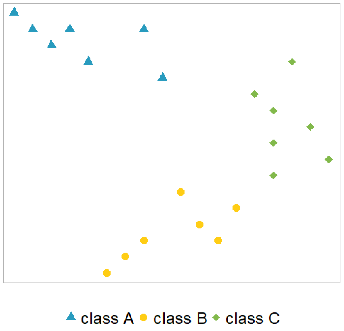
2. Modelling Multiple Status Transitions

In this section, we present different approaches to modelling multiple status transitions and focus on qualitative aspects of the model selection: we differentiate with respect to the structure, uniqueness, complexity of the model and the possibility to generalise to an arbitrary number of transitions. We also analyse and compare approaches to considering the history of an insurance contract in a model. This section focuses on the architecture of the different modelling approaches, while the specific implementation and application for our data set are described in Section 3 and compared in Section 4.
In our analysis of a typical insurance portfolio, only annual status transitions are tracked. Therefore, the initial status at the beginning of a year and the status at the end of the year are recorded, and exactly one potential transition during the year can be further analysed and considered in a multi-class problem. In the literature, there are several model structures for multi-class response variables where an estimated probability for each potential class is derived, and there are basically two ways of modelling such a multi-class problem: Firstly, decomposition strategies transform the original multi-class problem into several binary problems and subsequently combine them to obtain a multi-class model. Those approaches are particularly interesting for machine learning models like support vector machines, which were originally designed for binary problems. In the GLM framework, the binary model corresponds to logistic regression. An overview of decomposition strategies is given in Lorena et al. (2008). The decomposition strategies used for this analysis are described and discussed in Section 2.1, Section 2.2 and Section 2.3. Secondly, models with a holistic strategy can handle multiple classes directly with no need for decomposition. In the GLM framework, this corresponds to an MLR, as described in Frees (2004). This approach is described in Section 2.4.
In the analysis of policyholder behaviour, the transition history may impact future transition probabilities, e.g., the lapse probability may be increased for a contract that was paid up recently compared to a contract that has been paid up for a longer time. Therefore, different approaches of including the history in the model are discussed in Section 2.5. These approaches can be applied to both the decomposition approaches and the holistic approach.
For recurring terms, we use the following notation:
  • K is the set of possible classes for the response variable Y with m = | K | potential classes.
  • Based on Allwein et al. (2000), M corresponds to a coding matrix with possible entries, m i , j { 1 , 0 , 1 } . Each column, j, corresponds to a binary base model, indicating whether the class (in row i) has a positive label ( m i , j = 1 ), has a negative label ( m i , j = 1 ) or is not included ( m i , j = 0 ). The latter means that data from class i are not reflected in the calibration of model j.
  • p I : = P ( Y I | x ) describes the (predicted) probability that an observation, x, is in the subset of classes I.
  • x J denotes the subset of the observations, where y J .
  • p I J : = P ( Y I | x J ) .
  • In general, p describes a (predicted) probability from a binary model, i.e., before aggregation, and q describes a (predicted) probability for a multi-class model, i.e., after aggregation.
Hypothetical example:We illustrate each model with a hypothetical data set with three classes ( K = { A , B , C } and m = 3 ) for the response variable Y K and two not-further-specified covariates, X 1 and X 2 (adopted from Z. Zhang et al. 2016); see Figure 1. Each observation, ( x i , y i ) , in this example is depicted in the two-dimensional plane (covariates), where each class (response) is visualised using a different colour and symbol.

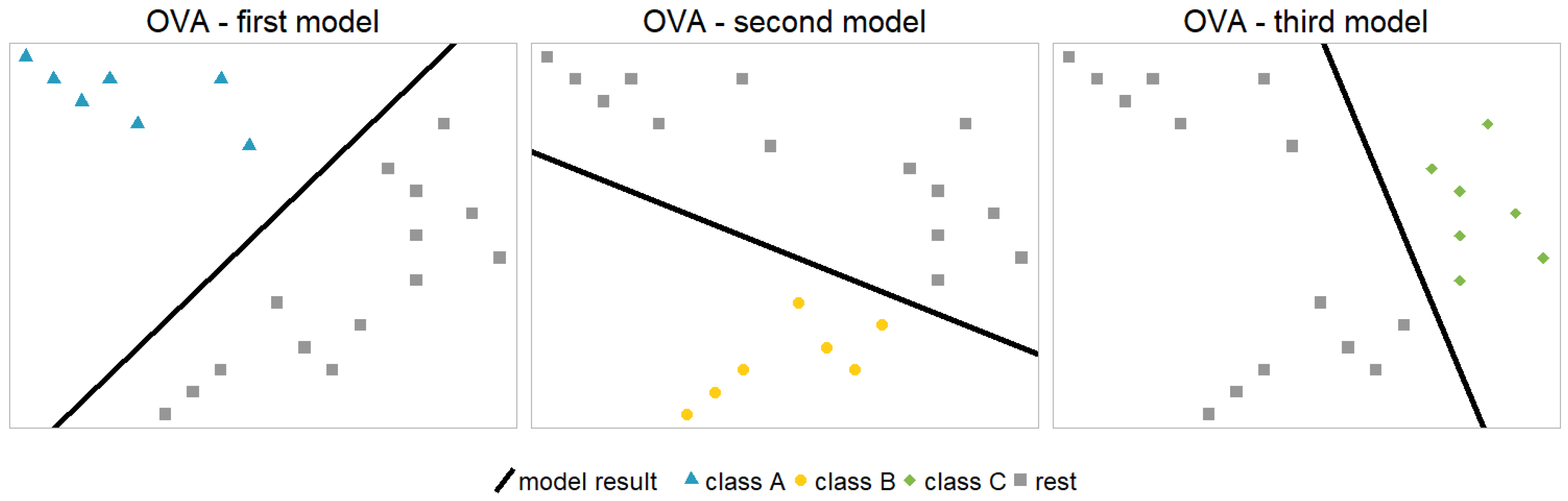
2.1. One vs. All Model

The one vs. all (OVA) model (also called one against all (OAA)) is a popular choice among the decomposition strategies. As the name suggests, the OVA approach builds several binary models; each models one class versus all the other classes:
M OVA = 1 1 1 1 1 1 1 1 1 .
Figure 2 shows the model architecture for the hypothetical example. The black lines represent binary model results separating the two relevant classes using the two covariates.
An aggregation scheme is necessary to transform the probabilities from the binary models into a multinomial model with probabilities for each class1. Note that the models themselves are unbiased in the sense that the average predicted value equals the average observed value. Therefore, the average predicted values of the individual models add up to one. However, this is not necessarily valid for a single observation, and in general, the sum of the predicted probabilities is not equal to one here. An intuitive approach for the aggregation is a rescaling of the individual probabilities, such that the original ratios are conserved, but the probabilities also add up to one for each single observation:
q i = p i i p i
This aggregation scheme is also statistically motivated since the rescaled probabilities, q i , are closest (in terms of the Kullback–Leibler distance; see Kullback and Leibler 1951) to the individual probabilities, p i , while adding up to one:
min q i p i log p i q i , s . t . i q i = 1 .
There are also other possible aggregation schemes.
For the OVA model with the rescaling aggregation scheme, there are m binary models that have a unique definition and are independent of each other. However, the aggregation scheme implies a dependency on the actual target, q. Thus, a prediction for a specific class may impact or even worsen the predictions for other classes.

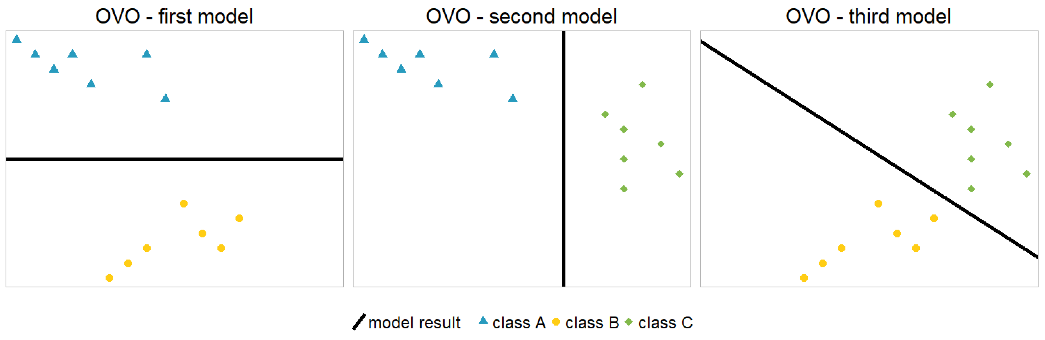
2.2. One-vs.-One Model
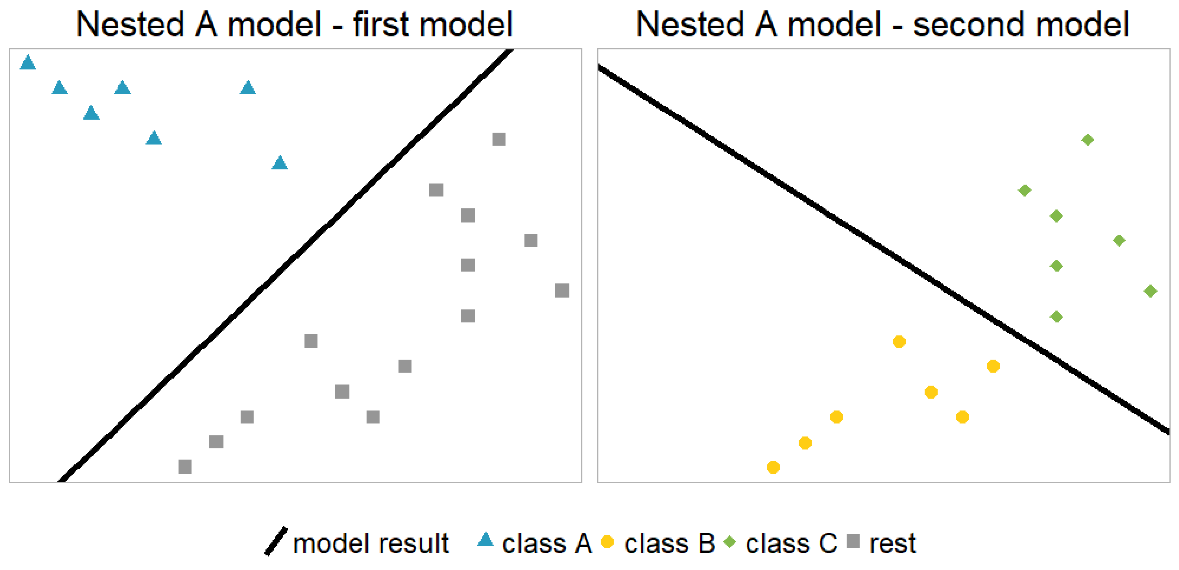
The one-vs. -one (OVO) model (also called one-against-one (OAO)) is another popular choice among the decomposition strategies. As the name suggests, the OVO approach builds several binary models; each models one class versus another class:
M OVO = 1 1 0 1 0 1 0 1 1 .
Figure 3 shows the model architecture for the hypothetical example. Again, an aggregation scheme is necessary to obtain a multinomial model with probabilities for each class2. There are several possibilities on how to aggregate the probabilities from the individual binary models, p i J , in order to estimate the probability distribution of the underlying data set, q i ; see Galar et al. (2011). Also, note that the individual models in the OVO approach can ‘contradict’ each other in the sense that there is no compatible set of probabilities, q i ; e.g., if p A A , B = 0.9 , p B B , C = 0.8 and p A A , C = 0.2 . In this analysis, we apply pairwise coupling, as proposed by Hastie and Tibshirani (1997) for the aggregation. The idea is to minimise the (weighted) sum of the Kullback-Leibler distances between p i i , j and μ i , j = q i q i + q j , where the weights w i , j correspond to the number of observations in x i , j :
min q i < j w i , j p i i , j log p i i , j μ i , j + p j i , j log p j i , j μ j , i
For the example above, where p A A , B = 0.9 , p B B , C = 0.8 and p A A , C = 0.2 , the proposed aggregation scheme (with w i , j = 1 i , j ) gives q A = 0.38 , q B = 0.29 and q C = 0.33 . Since the individual models would imply that A is more likely than B, and that B is more likely than C, but then that C is more likely than A, the aggregated probabilities around 1 3 seem reasonable. The order q A > q C > q B appears plausible as well since the combined estimated probabilities from the individual models are 1.1 > 1.0 > 0.9 for classes A , C and B.
An alternative and intuitive aggregation scheme for the OVO approach is the rescaling of the combined estimated probabilities, such that the resulting probabilities add up to one. In the example above, this would lead to q A = 1.1 3.0 = 0.37 , q B = 0.9 3.0 = 0.30 and q C = 1.0 3.0 = 0.33 . Even though the resulting probabilities (for this example) are very similar to those from the pairwise coupling, the alternative aggregation scheme performed significantly worse in the comparisons, as laid out in Section 4. Therefore, we decided to omit this alternative aggregation scheme and focus on pairwise coupling even though the interpretability of the OVO approach suffers from the rather complicated aggregation scheme.
The number of necessary binary models increases rapidly with the cardinality of K. In general, there are m ( m 1 ) 2 models in the case of m classes for the response variable, and the individual models are independent for the sub-samples. As for the OVA, the aggregation scheme implies a dependency on the actual target, q.

2.3. Nested Model

Nested models (also called hierarchical models) are another example for combining binary models to arrive at a multinomial model. OVA and OVO are symmetric in the sense that changing the order of the classes does not impact the result, i.e., these models have one unique definition. Within the nested approach, there are multiple ways of defining the hierarchical model setup. For example, in the case of three classes, there are three possible model architectures:
M Nested A = 1 0 1 1 1 1 , M Nested B = 1 1 1 0 1 1 , M Nested C = 1 1 1 1 1 0 .
Figure 4 shows the first model architecture (Nested A) for the hypothetical example.
In general, there are many separation possibilities; see Equation (8) below. In each step of the hierarchy, the remaining classes are split into two (potentially imbalanced) parts until, finally, each class is separated. Therefore, each individual class, k, has subsets, j i , describing the unique separation path of length s: K = j 0 j 1 , j s 1 j s = k .
The hierarchical design of the aggregation scheme ensures well-defined probabilities, and thus, an aggregation scheme is not necessary for the nested approaches. To obtain the prediction of a class, we use the specific path for that class:
q k = i = 0 s 1 p j i + 1 j i .
The specific order is rather arbitrary and has a major impact on the complexity of the prediction, q k . We will see in Section 3 that this order also affects the quality of the model fit tremendously. This dependency on the order is a major disadvantage of the nested models. In some applications, expert judgement can help identify a reasonable order. In many applications, however, the best possible order is a priori unknown.
In general, there are m 1 models in the case of m classes for the response variable, as for the OVO approach. However, this time, the order matters. The models are not independent since, in each step of the hierarchy, the models are conditioned on the result of the higher levels of the hierarchy. We have seen in the hypothetical example that, for three classes, only three different orders are possible. But, with four classes, there are 15 possible orders, and with five classes, they are already 105. To obtain a general formula for the number of possible orders, we derived a recursive formula based on combinatorial terms and then transformed it into the following compact representation using the gamma function:
f ( m ) = 2 m 1 Γ ( m 1 2 ) π ,
where f ( m ) is the number of possible orders for m final classes.
Thus, there is potentially a huge number of possible model specifications and a high complexity introduced via the number of binary models.

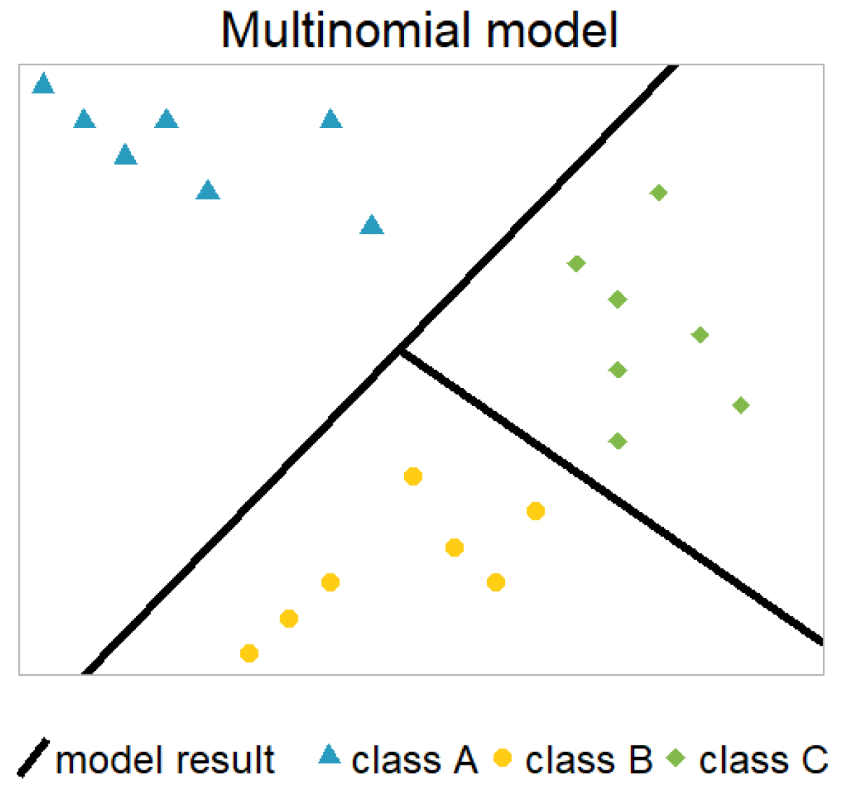
2.4. Multinomial Model

Instead of decomposing the multi-class problem into several binary problems (e.g., using the OVA, OVO, or nested methods), we can also approach the multinomial problem directly. Within the GLM framework, the most intuitive way is to use an MLR, which is a direct generalisation of the logistic regression; see Frees (2004). Figure 5 shows the model architecture for the hypothetical example. Also, outside of the GLM framework, there are several algorithms capable of modelling multiple classes, e.g., neural networks with a softmax layer or random forests.
The MLR estimates all probabilities simultaneously. Therefore, we do not need to transform individual probabilities using an aggregation scheme as before. The black line in Figure 5 represents a hypothetical model to separate the classes—this time, three classes simultaneously, instead of just two classes at a time.
This approach only uses one model, no matter how many states the response variable has. Hence, it uses all information simultaneously for the prediction of an observation. The model structure is unique; therefore the model imposes a significant complexity reduction.

2.5. Transition History

There are many applications—including ours—where observations are made over time. In our data set (see Section 3.1), this corresponds to a yearly observation for each in-force contract. At the end of each complete contract year, the current state is tracked (it can be active, paid-up, or lapse). Therefore, we do not differentiate between, for example, lapse after 4.5 contract years or 4.8 contract years. The remaining covariates do not change over time. This results in a sequence of possible states and transitions for each observation. The transition history of an observation may impact the probabilities of future transitions, e.g., the lapse probability may be increased for a contract that was paid up recently compared to a contract that has been paid up for a longer time. In order to improve estimates of transition probabilities, it may be useful to consider the past of an observation in the model. There are several ways to include the transition history in the model, and we focus on the following three approaches:
  • No previous information: There is always the possibility of ignoring any information about previous states. This is the easiest and most primitive way of dealing with the transition history but, it can still be legitimate for applications where the history is obviously irrelevant.
  • Markov property: A Markov property can be assumed, see Dynkin (1965). The ‘past’ (transition history) does not matter for the ‘future’ (predictions), given that the ‘present’ (current state) is known, i.e.,:
    P ( Y t = y t | Y t 1 = y t 1 , Y t 2 = y t 2 , , Y 1 = y 1 ) = P ( Y t = y t | Y t 1 = y t 1 ) ,
    where t indicates the time (=contract duration) of an observation and Y t corresponds to the state (active, paid-up, or lapse) in that year, t. Hence, we are modelling yearly lapse and paid-up rates.
  • Full transition history: There are also applications in which it is possible to define one new covariate (or more), which represents the state history sufficiently. This highly depends on the number of states and the structure and dependencies of the underlying data set. In our specific example, the time since paying up seems to sufficiently describe the state history; see Section 3.1 for details.
In the second and third approaches, there is still flexibility in how to include the information in the model. Let the status history be sufficiently described in one (or more) new covariates, X h i s t o r y . Subsequently, it can be treated as a normal covariate in the model. Alternatively, the covariate and all its interactions with the remaining covariates can be included in the model. This allows the model to identify more complex structures in the data. A third way is splitting the data according to that covariate and building separate models for each subset. Note that this increases the number of individual models for each model architecture. Including the covariate in the model formula is no longer necessary since it is just constant for each subset. However, in cases where the history can only be captured sufficiently using many new covariates, or if the number of possible classes is high, this third approach may not be feasible.
All above-mentioned approaches are analysed for our data set in Section 4.

3. Application for a European Life Insurer

In this section, we further specify, apply, and compare the approaches to modelling multiple status transitions for a portfolio of life insurance contracts provided by a pan-European Insurer operating in four countries. An elaborate description of the considered models can be found in McCullagh and Nelder (1989) for GLMs, in R. Tibshirani (1996) for the Lasso, in R. Tibshirani et al. (2005) for the fused Lasso, and in Kim et al. (2009) for the trend filtering. Also, see Reck et al. (2023) for the application of the extended versions of the Lasso to a logistic lapse model.

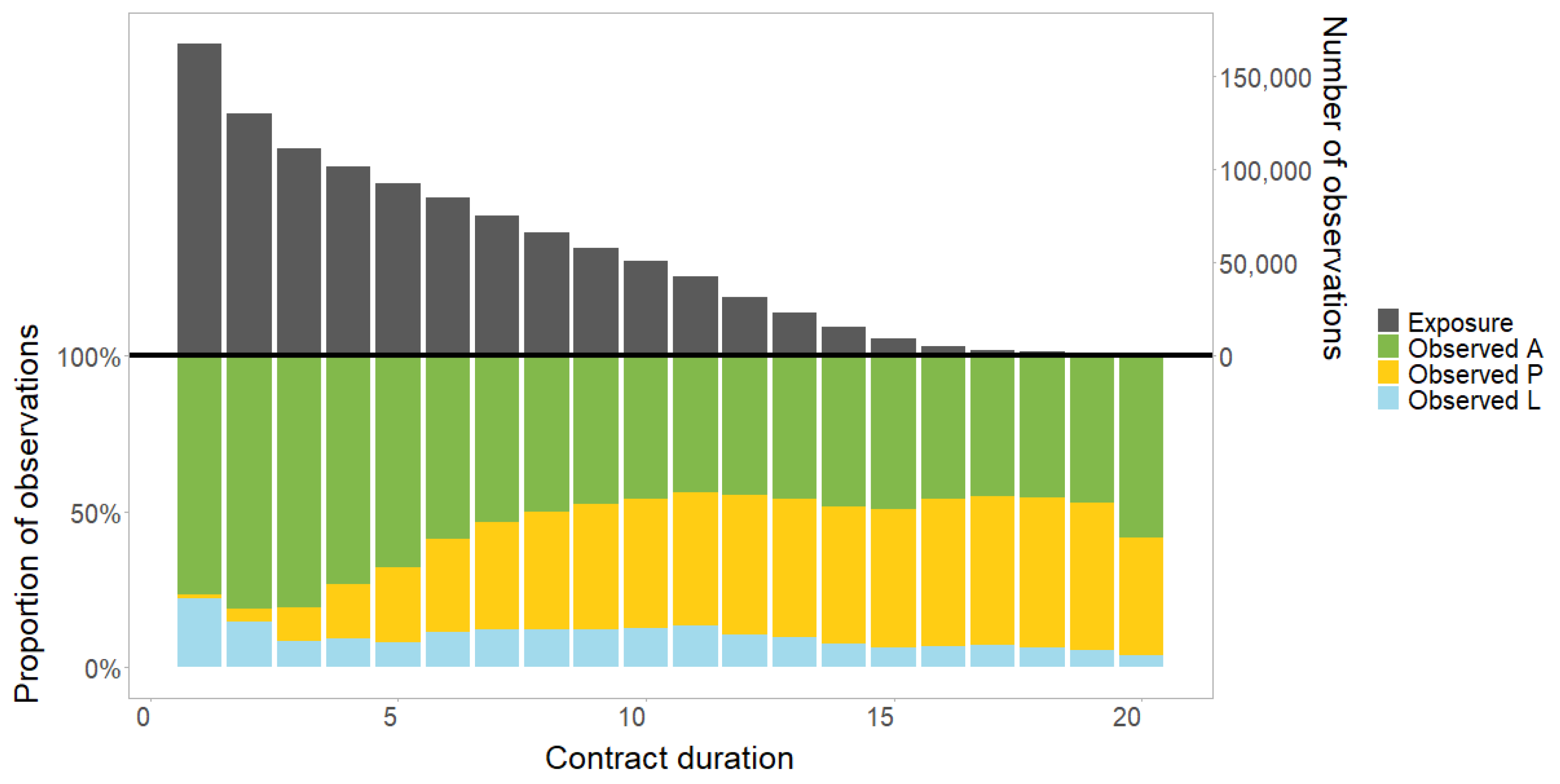
3.1. Data Description

The data set contains a large number of insurance contracts over an observation period of around 21 years. This particular portfolio went into run-off after about 11 years, which means that no new contracts were written after that. Nevertheless, the insurer is required to fulfil the regulatory requirements (and the estimation of the best estimate transition rates are essential for that) until all contracts have expired. Also, the insurer does not aim to transfer the business to an active portfolio, as it is specialised in run-off business. The fact that this portfolio went into run-off does not affect the proposed modelling approaches—they can also be applied to portfolios that are not in run-off. However, this should be kept in mind when interpreting the coefficients in Appendix A. The data set comes from a single source, is well structured, and does not contain any missing values. It is treated confidentially, as it contains customer and company-related information.
Life insurance contracts typically include several options available to policyholders, such as full surrender (lapse) and the stopping of regular premium payments (paid-up), but they also include the option for the reinstatement of premium payments after paying up, partial surrender, pre-defined dynamic premium increases and other premium increases, or the payment of top-up premiums. For the contracts in this particular portfolio, the key observed status transitions of the contracts are the option of paying up a contract and the exercise of a full surrender (lapse) option. Thus, the data set appears well suited to applying the presented models using three possible states: active (A), paid-up (P), and lapse (L). Note that, for other portfolios, significantly more transitions may need to be modelled.
In this paper, the option to ‘lapse’ is defined to comprise surrender (the policyholder cancels the contract and gets the surrender value), pure lapse (the insurance contract is terminated without a surrender value payment), and transfer (the policyholder cancels the contract and transfers the surrender value to another insurance company). The second option, ‘paid-up’, is defined by a reduction in the regular premium payments to zero, but the contract remains in force. Obviously, an execution of the first option implies a transition to a terminal status. The paid-up option leaves a potential lapse option open in the future.
There are n = 1,070,139 observations (167,659 unique contracts) with an extended set of up to J = 15 covariates: contract duration (the number of years between inception and observation time), insurance type (traditional or unit-linked), country (four European countries), gender, payment frequency (e.g., monthly or annually), payment method (e.g., debit advice or depositor), nationality (whether or not the country, in which the insurance was sold equals the nationality of the policyholder), the dynamic premium increase percentage, entry age, the original term of the contract, the premium payment duration, the sum insured, and the yearly premium. Other specifications about the insurance type (other than traditional or unit-linked) are not available in our data set and could, therefore, not be included in the model calibration. A finer distinction (e.g., term life, whole life, the existence of riders, etc.) can provide further interesting insights. Moreover, options like top-ups and premium holidays are not material for this run-off portfolio, as they are rarely observed. This could be material for other life insurance portfolios.
We extend this original set of covariates by including two covariates that contain information about the previous state (or states) of a policyholder. For some models, we only consider the previous status (i.e., active or paid-up, since lapse is the terminal status). For other models, we also add another covariate, time since paying up, which counts the years between being paid up and the observation time. It is defined as 0 as long as a policyholder is still active (of course, each policyholder initially starts in the active state). For this data set, there are no observations with reinstatement, meaning that we do not observe the transition P → A. Other covariates do not change over time and are, therefore, deterministic for our life insurance portfolio. Hence, the covariates’ contract duration and the time since paying up uniquely determine the full state history of a contract3.
For modelling purposes, a separate row is created for each in-force contract in each observation year. As a consequence, one single contract may occur in several rows in the data set—once for each observation year when the contract is still in force. This differs from a standard survival analysis setup, where we would typically have one observation per contract. This observation would then contain information about the duration (until being paid up and until lapsing), potential censoring, and the final state. This modification leads to a data set where the rows are no longer fully independent, and we also have a selection bias (contracts being in force longer get more weight than contracts lapsing early). Given the size of our data set, this modification seems justifiable. However, in general, the effect of this modelling approach should be analysed carefully.
Figure 6 shows the decreasing exposure (upper part) and the composition of the three states (lower part) for different values of contract duration. The one-year lapse rates clearly decrease rapidly in the first three years, which is consistent with the well-known higher lapse rate at the beginning of an insurance contract. The one-year paid-up rate shows a different trend: starting with a very small percentage for the first year of the contract, the rate increases over time until it reaches a certain threshold. Although the rates have different trends, they should be modelled consistently together.
The calendar year might contain valuable information about policyholder behaviour, e.g., with higher lapse rates during a financial crisis (emerging fund hypothesis). To quantify the calendar year effect, we add a new covariate in a sensitivity analysis for one of the qualitatively and quantitatively best models. The results are discussed and evaluated in Section 4.2. For future transition rates, however, the calendar year effect is unknown a priori, and therefore, further assumptions are required to derive a best estimate.
Other macroeconomic indicators for a specific calendar year, like the swap rate, inflation rate, or stock performance, or demographic indicators for a specific country, like the social security system, might contain helpful information for many portfolios. However, since previous research suggests that they turn out to be not significant on this particular data set (see Reck et al. 2023), we refrain from a deeper evaluation in this analysis.
One useful pre-processing step in this framework is the binning of continuous covariates. With that, the corresponding covariate has several pre-defined category levels (bins). Without binning, the model can either estimate a single parameter for the continuous covariate (and potentially underfit) or estimate a parameter for every single value of the covariate by treating it as a factor (and potentially overfit). With binning, we are, therefore, able to derive an interpretable model with good predictive power to satisfy the requirements of an insurance company.
There are different possibilities for choosing adequate bins, e.g., bucket binning (each bin has the same length), quantile binning (each bin has the same number of observations), or simply relying on expert knowledge. There are also more complex ways to define bins: Henckaerts et al. (2018) use evolutionary trees as described in Grubinger et al. (2014) to estimate optimal bins for continuous variables. These evolutionary trees incorporate genetic algorithms into the classical tree framework to find the global optimum by also allowing changes in previous splits. We choose a rather simple data-driven approach (no expert knowledge) to derive the bins and follow the approach of Reck et al. (2023) using a univariate decision tree for each continuous covariate in the data set: the entry age, the original term of the contract, the premium payment duration, the sum insured, and the yearly premium. To avoid overfitting, we use small trees with at least 5% of the observations in each terminal leaf (see again Reck et al. 2023). Note that contract duration is not assumed to be continuous, and no univariate decision tree is built. The category levels are, therefore, just the natural numbers up to 20.

3.2. General Model Setup

Since we are looking for a parsimonious and interpretable model, we focus on GLM-based models using extended versions of the Lasso in our analysis. The probabilities are defined as follows:
P ( Y = 1 | x ) = e x T β 1 + e x T β , P ( Y = k | x ) = e x T β k l = 1 m e x T β l ,
where Y is the target variable, x is the covariate vector, and β is the model parameter vector. The first equation corresponds to the logistic regression (the binary case of the decomposition strategies), and the second equation corresponds to the MLR with m classes. The logistic regression is a special case of the MLR with m = 2 . However, in Equation (10), the reference level for the logistic regression is implicitly set to one of the two classes, while there is no explicit reference level for the MLR. Consequently, we only consider those coefficients not corresponding to class A in the results to make the comparison of the number of coefficients in the models fair.
For the logistic regression, we have the following log-likelihood function:
log Likelihood ( β | x , y ) = 1 n i = 1 n y i ( x i T β ) log ( 1 + e x i T β ) .
The parameters β are estimated with a penalised maximum likelihood optimisation (regularisation). We use the methodology proposed by Reck et al. (2023):
log Likelihood ( β | x , y ) L a s s o = log Likelihood ( β | x , y ) + λ j = 1 J g P e n j ( β j ) ,
where λ controls the penalisation strength ( λ = 0 corresponds to a regular GLM without penalisation, and higher values for λ correspond to a higher penalisation and, therefore, fewer parameters), and P e n j represents different versions of the Lasso, i.e., a regular Lasso, a fused Lasso, and trend filtering:
g R ( β j ) = i = 1 p j | β j , i | = : i = 1 p j | β j , i R | , g F ( β j ) = | β j , 1 | + i = 2 p j | β j , i β j , i 1 | = : i = 1 p j | β j , i F | , g T ( β j ) = | β j , 1 | + | β j , 2 2 β j , 1 | + i = 3 p j | β j , i 2 β j , i 1 + β j , i 2 | = : i = 1 p j | β j , i T | .
The regular Lasso penalises the difference of each category level to the intercept ( | β j | ) and can be used for covariates without ordinal scale. The fused Lasso penalises the difference between two adjacent category levels ( | β j β j 1 | ) and is, therefore, suitable for fusing neighbouring category levels. Finally, the trend filtering penalises the difference in the linear trend between category levels ( | β j 2 β j 1 + β j 2 | ). It is, hence, used to model a piecewise linear and often monotone structure within that covariate. For trend filtering, we start with the middle category level as the intercept, as this category has a material exposure in any case. For the MLR, the equations can be adjusted according to the following:
log Likelihood ( β | x , y ) = 1 n i = 1 n l = 1 m y i , l ( x i T β l ) log ( l = 1 m e x i T β l ) ,
and
log Likelihood ( β | x , y ) L a s s o = log Likelihood ( β | x , y ) + λ j = 1 J l = 1 m g P e n j , l ( β j , l ) .
These extended versions of the Lasso allow the model to capture structures within covariates—however, only for the effect on a specific value of the response variable. A penalisation across different values of the response variable is not possible in this modelling setup. For example, two different coefficients for the effect of a covariate, j, on lapse, β j 1 , L and β j 2 , L , may be fused together. Similarly, the two different coefficients for the effect of covariate j on paid-up β j 1 , P and β j 2 , P may be fused together. However, a fusing between β j 1 , L and β j 1 , P or between β j 2 , L and β j 2 , P is not possible. To our knowledge, this form of optimisation has not been implemented yet.
For the implementation, we essentially use the same setup as described in Reck et al. (2023), which can be summarised by
  • Using the R Core Team (2022) interface for the h2o library—see LeDell et al. (2022);
  • Modelling the trend and fused Lasso penalty with contrast matrices;
  • Determining the hyper-parameter λ based on a 5-fold cross-validation using the one standard error (1-se) rule4.

3.3. Specific Model Setup and Parameter Estimation

For the decomposition strategies, Equation (12) can be applied for each binary model independently, based on the coding matrices, M. This results in the calibration of three independent binary models (see M OVA and M OVO ) or two independent binary models (see M Nested A , M Nested B and M Nested C ). Therefore, we perform three (two) independent penalised maximum likelihood estimations using Equation (12) with corresponding λ i and β i . The calibration of the binary models is independent, and therefore, the values of penalisation terms differ in general; see Table 1. In contrast, the MLR only requires a single model calibration using Equation (15).
Table 1 shows the main findings with respect to the penalisation term λ :
  • The second model of each nested approach is identical to a model in the OVO approach. Of course, this can also be seen when comparing the columns of M O V O in Section 2.2 with M Nested A , M Nested B and M Nested C in Section 2.3.
  • Splitting the data set requires an additional model which is identical for all approaches (cf. the last entry in the last column). For the subset with the initial state ‘active’, the number of models is identical to the previous number of models (including both initial states) because the corresponding response variable can still have all three states, ‘active’, ‘paid-up’, and ‘lapse’. For the subset with the initial state ‘paid-up’, however, one additional model is required with possible levels ‘paid-up’ and ‘lapse’ for the response variable. It is just a single logistic regression with an initial state, ‘paid-up’, and response, ‘paid-up’ or ‘lapse’.
  • Whenever a model distinguishes class P from one (or all) other classes, the corresponding λ value is rather high—especially when P and L are compared (see Nested A, second model). A plausible interpretation might be that separating class P is comparably easy for a model in the sense that the model performance does not decrease when the penalisation is increased.
  • The decomposition strategies have a higher degree of freedom in terms of the λ value because they might differ for the individual binary models. In this application, however, the λ values seem to have a similar magnitude across the different modelling approaches. Note that we also optimised the penalised likelihood functions from the decomposition strategies with the restriction of a constant penalisation term, λ i , for all binary models. As expected, the impact on the results was rather small. This might be different in applications where the independently calibrated values vary more. In the end, we chose the penalisation terms of Table 1, which is consistent with the independent model definitions.
In principle, P e n j , l may also differ for the individual binary models within a decomposition strategy. This again leads to a high degree of flexibility; e.g., if P e n entry age , A = ‘trend filtering’ and P e n entry age , P = ‘fused’. However, this flexibility did not seem to impact the result significantly, such that we chose the same penalty type for all models, as described in Table 2. The different penalty types allow the model to identify different structures within covariates, as described in Section 3.2. The choice of the appropriate penalty term, therefore, highly depends on the structure of the corresponding covariate. For more details and the mathematical matrix representation, we refer to Reck et al. (2023) or R. J. Tibshirani and Taylor (2011).
Finally, the estimated coefficients are fed into Equation (10). For the decomposition strategies, the resulting probabilities are then transformed using the aggregation schemes presented in Section 2. For the MLR, the resulting probabilities are directly well defined and do not require further modifications.

4. Results and Comparison of the Modelling Approaches

After we have described the different modelling approaches, as well as the calibration to the underlying data set, we now analyse and compare the results. We focus on two dimensions: the different model architectures (see Section 2.1, Section 2.2, Section 2.3 and Section 2.4) and the inclusion of the transition history (see Section 2.5). We have seen that, due to their architecture, some of the models require considerable effort and readjustment to generate multinomial probabilities. Therefore, we also include the complexity (number of models and number of parameters) and the computing time of the models as additional components that are obviously important for the model selection.
Table 3 shows the two dimensions of the analysis: the rows show different model architectures, and the columns show different ways of including the transition history. Reck et al. (2023) also analyse further perspectives in a sensitivity analysis. They find that the Lasso approach offers advantages with respect to performance compared to univariate approaches like Whittaker–Henderson. It also has advantages with respect to the model complexity (measured with the number of parameters) without a loss in performance compared to a GLM. The latter is also true for ridge regression and the elastic net. We expect similar results for this analysis.
Furthermore, the extended versions of the Lasso (regular, fused, and trend filtering) allow for differentiated modelling of structures within covariates without adding too many parameters to the model. Hence, the selective property of the Lasso omits bins or category levels from the model. The choice of λ using the 1-se rule also supports the selection of a robust model with competitive performance.
The table is split into three parts: the upper part shows the performance of the models. The performance measure is defined as 1 D m D 0 , where D m corresponds to the deviance of the model, and D 0 corresponds to the deviance of the intercept-only model (or null model). Therefore, it can be interpreted as the relative improvement over the intercept-only model. This measure is similar to the R 2 measure for normally distributed response variables, with a similar interpretation. Since the measure is based on deviance, it is also consistent with the likelihood optimisation described in Section 3.2. Other performance measures (e.g., the multi-class area under the curve (AUC) as defined by Hand and Till 2001) show a similar pattern. The middle part of the table shows the number of models, the number of parameters, and the number of potential parameters. An entry, a , b / c , thus means that a individual models were built to get the overall prediction, and a total of b parameters were selected via the underlying Lasso out of c possible parameters from the underlying data set (or data sets). Parameters where the Lasso assigns a value of zero are not included in this entry b, as they implicitly disappear from the model. The lower part of the table shows the computing time (in minutes) on a standard computer. The aggregation scheme for the OVA model is very simple, so there is no measurable effort here. For the OVO model, however, the aggregation effort is considerable. For this model, the aggregation effort is given in parentheses.
Figure 7 visualises a part of the information from Table 3. The different models (except the intercept-only model) are visualised by colours, and the different transition histories are visualised by shapes. The x-axis shows the number of parameters, and the y-axis shows the relative improvement over the intercept-only model.

4.1. Transition History

Markov property (vs. no previous information): We can clearly see in the figure (or in the Markov property column) that the previous state contains valuable information. All models perform significantly better with the previous state compared to the corresponding model without any previous information (between 8 and 17 percentage points). This is intuitive since the fact that a contract was already paid up before impacts the chance of it being paid up in the current year. Since only one potential coefficient is added to the model ( β p r e v i o u s s t a t u s ), the number of parameters does not change a lot (all changes within plus and minus 15%) and for most of the models even decreases, e.g., from 112 to 103 for Nested L. This is an indicator that the additional covariate β p r e v i o u s s t a t u s contains valuable information such that other covariates are then no longer required in the model. Of course, this highlights one of the major advantages of using the Lasso approach: it selects the covariates automatically.
Full transition history (vs. Markov property): The full transition history, including the time since paying up, does not seem to improve the model significantly. Even though it increases the number of parameters (e.g., by 31% for the Nested L), the deviance is equal to or only marginally better than the deviance of the model with only the previous state (all changes less than half a percentage point). This holds true for all models. Therefore, the time since paying up does not seem to add value to the model - as long as the previous state is included.
Markov property with interaction (vs. Markov property): When using the previous state, including its interaction terms, the performance is somewhat better than that of the corresponding model without interactions (up to 2.2 percentage points). This illustrates the selective property of the Lasso: Models with these interaction terms are able to recognise different structures for the impact of a covariate on the target variable, depending on the initial state. However, the number of parameters increases significantly (e.g., almost doubles for the MLR). This is not surprising, as an interaction term is included for every covariate, i.e., the number of potential parameters is essentially doubled (the previous state can be A or P). If the number of initial states increases further, the number of interaction terms increases accordingly.
Markov property with splitting (vs. Markov property): Using the previous state by splitting the data set also seems to perform somewhat better than the corresponding model using the previous state as a covariate (up to 2.1 percentage points). The number of parameters seems to be on a similar level (some are higher; some are lower). Note that there is always one additional model when splitting the data set. As described above, this additional model is exactly the same for all modelling approaches.
Markov property with splitting (vs. Markov property with interaction): In terms of model performance, there is no material difference between splitting of the data set and allowance for interactions (a decrease by 0.1 to 0.2 percentage points). However, the models based on splitting the data set have much fewer parameters (between c. 20% and 40%).
Qualitative comparison: We analysed and compared different alternatives for the inclusion of the transition history of a contract. Increasing the number of potential states, the first one (adding the previous state as a covariate) increases the complexity of the model only marginally. The second one (adding the previous state and its interaction terms) can also be generalised to more potential states—however, this increases the number of parameters significantly. The third one (splitting the data set) requires further splits and might not be feasible for many more states—especially when some states only show a few observations. The inclusion of the ‘full transition history’ in a single covariate is only possible for our specific example. In general, with an increasing number of states, several covariates are necessary to replicate the full transition history.

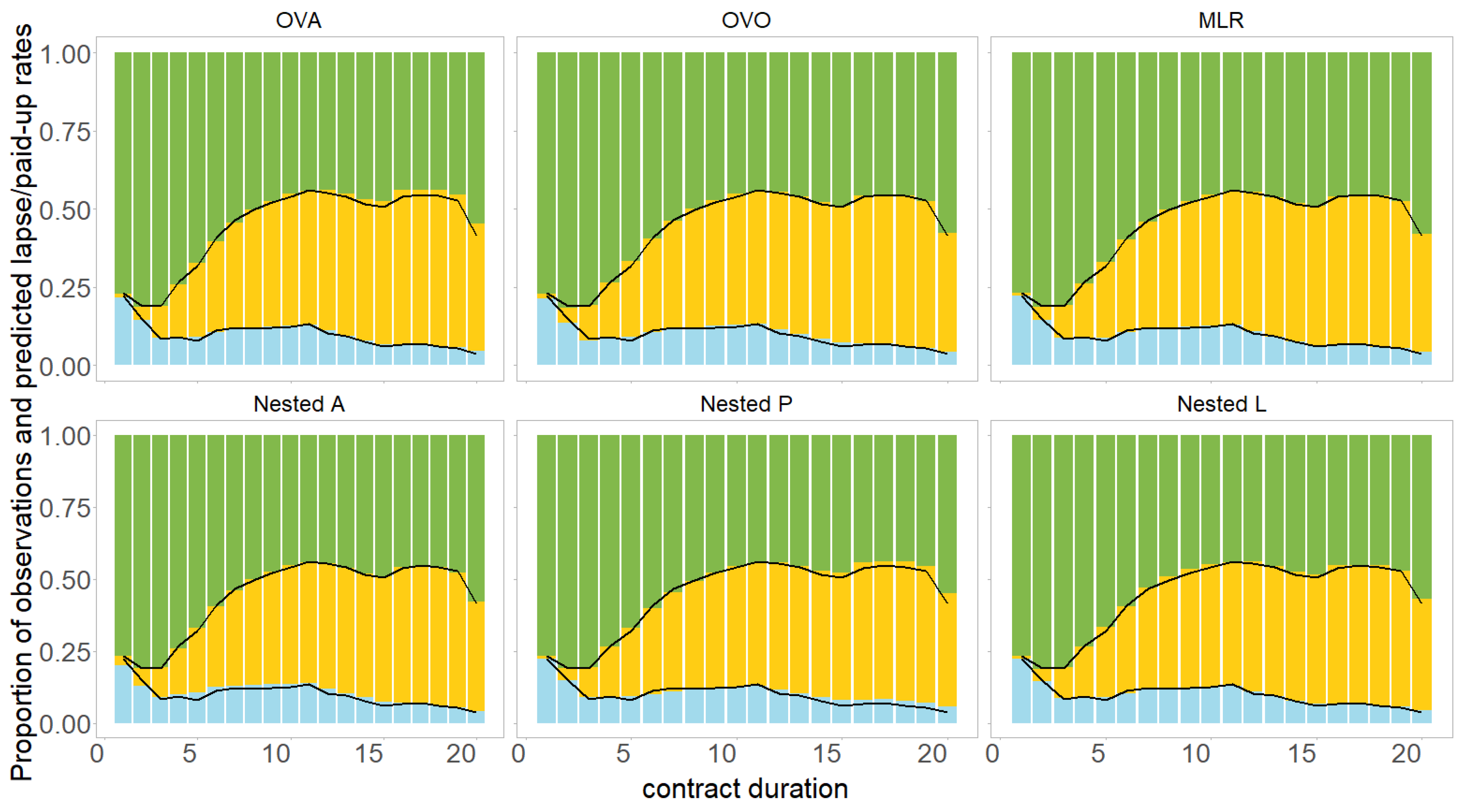
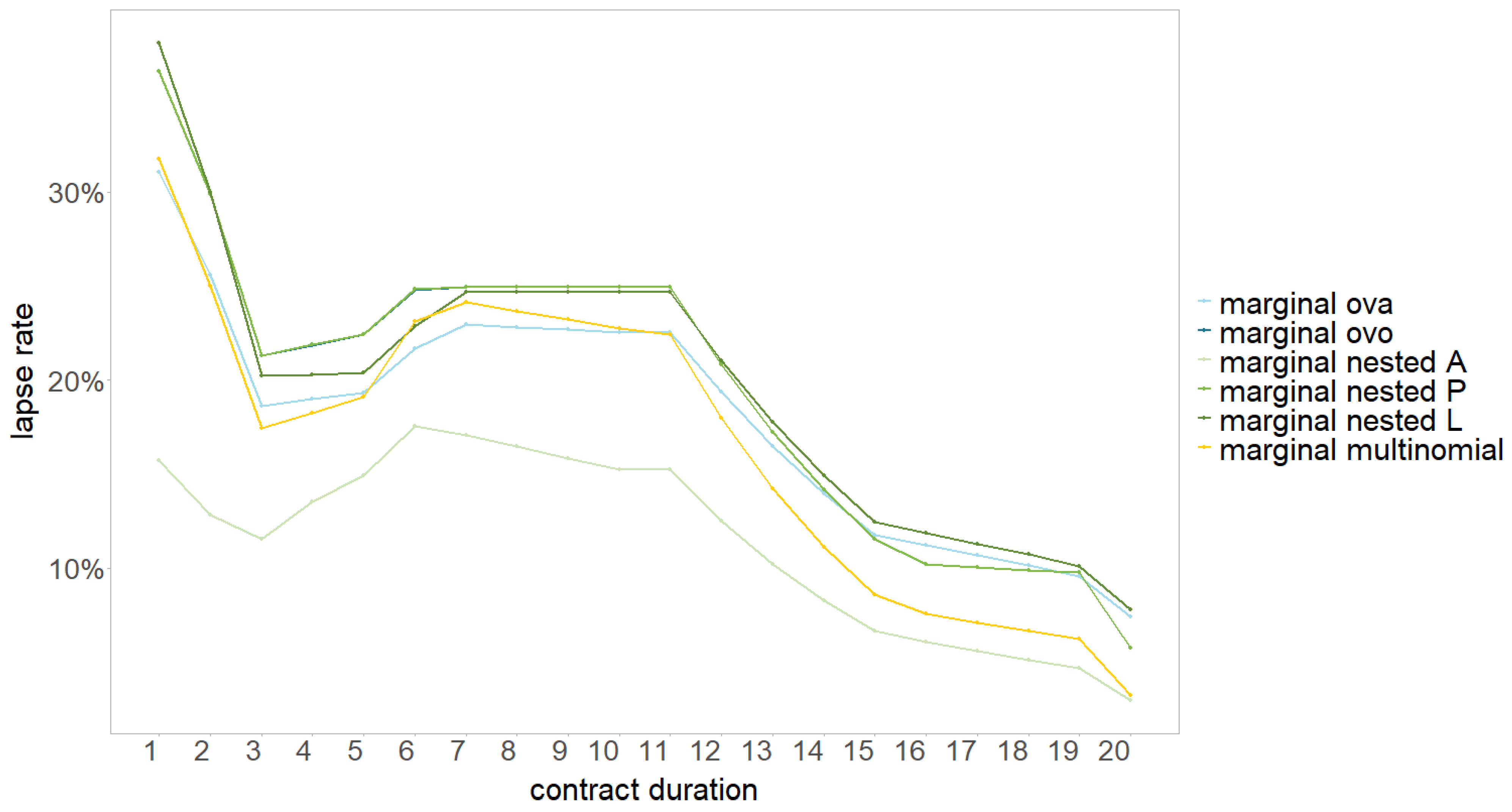
4.2. Modelling Approaches

Quantitative comparison: Overall, the different models show similar performances, e.g., in the range of 46.6–51.4% when including the previous state as a covariate. The OVO approach achieves the best deviance across different ways of including the transition history. Within the nested models, the order seems to play an important role for the performance. Without further empirical knowledge, Nested A may seem like a good choice, as the majority class is separated in the first step (actives vs. paid-up/lapse). However, this model performs the worst among all models. To find the best nested model, all possible orders have to be analysed, which can be very time-consuming. In this case, nested L performs the best among the nested models (first separating lapse from active/paid-up). The performance of the OVA, nested P, and MLR are similar in terms of deviance.
Figure 8 shows the predictions of the models (the black line) using a similar format as the lower part of Figure 6. All modelling approaches show a similar shape for the predicted lapse rate, i.e., a strongly decreasing trend for the first two contract years, followed by a constant or slightly increasing trend until year 11 before eventually decreasing again until year 20. The shapes of the predicted paid-up rates are also similar for the different models. The multivariate predictions (with respect to contract duration) are consistent for all approaches.
For the number of parameters, the MLR offers an advantage over the other approaches. After that, the nested models follow. OVO and especially OVA have the most parameters.
The computing time shows that the MLR is comparatively slow (it takes about twice as long as a nested case). The penalised maximum likelihood optimisation is based on a multinomial distribution here, compared to binomial distributions for the other approaches. Presumably, the numerical optimisation is more complex for MLR. The OVO model is a clear outlier due to the time-consuming aggregation that is much more expensive than the actual calibration of the binary models. Note that this aggregation must also be applied for each individual case so that the effort is also incurred in the application of the model and not only in the calibration. If the number of classes increases, we would expect a similar computing time for the multinomial model. For the decomposition models, however, the computing time is expected to increase rapidly.
Qualitative comparison: We now compare the qualitative aspects of the models: the complexity and interpretability of the model architecture, as well as the ability to generalise to more potential states. We also show the marginal effect of the models with respect to the covariate contract duration; see Figure 9. For that, we use the estimated coefficients for contract duration (and the intercept) in each individual model (and set all other coefficients to zero) to predict the individual probabilities. Then, we use the same aggregation scheme as for the overall prediction. Especially the OVO aggregation changes the interpretability of the individual probabilities significantly. The corresponding line, therefore, only partly reflects the overall model behaviour for the OVO. In general, the shape is similar for the models with a decreasing trend for the first three years, followed by a slightly increasing trend until year six. After that, there is a constant (or only slightly decreasing) trend until year eleven, followed by a clear trend change resulting in a decreasing trend until the end. The Lasso approach, therefore, decreases the number of parameters significantly by grouping certain category levels. For example, instead of the six original category levels 6, 7, 8, 9, 10, and 11 for contract duration, we might only need to consider one group 6–11 (depending on the modelling approach). Since we used the trend filtering for contract duration, one group follows one linear trend and between different groups are then trend changes.
It is also noteworthy that the marginal effect of the OVO approach is almost identical to the marginal effect of the Nested P model. This is due to the fact that the first and third models in the OVO approach, as well as the first model in the nested P approach, hardly use the contract duration as a predictor. Instead, they focus on other covariates (like β p r e v i o u s s t a t u s ), which are set to 0 for the marginal plot and are, therefore, omitted in the prediction. Thus, the two lines appear to be congruent. The OVA and OVO approaches have a rather simple architecture and are still easy to generalise. The number of required models is O ( m ) for the OVA approach and O ( m 2 ) for the OVO approach. Both approaches require an aggregation scheme to obtain the final probability for each class. The OVA aggregation scheme basically builds a weighted sum of the individual models and, therefore, remains fully interpretable. The OVO aggregation scheme is rather complex, such that there is no direct and interpretable connection between the final prediction and the individual predictions. This is a major disadvantage of the OVO approach.
The nested models have a more complex architecture. The order of the classes is critical here, which makes this approach unfeasible for situations with a higher number of classes. This can be seen in Figure 9, as the marginal effects for the nested approaches differ significantly. Therefore, the generalisation to more potential states is not trivial. The number of possible orders is O ( 2 m m ! ) , and the number of required models for each order is O ( m ) . Although the aggregation scheme seems rather intuitive, the multiplication of models complicates the model interpretability. Thus, the nested approach has a qualitative disadvantage in terms of the loss of generalisation and interpretability.
The MLR offers the most qualitative advantages: It is a single model (i.e., O ( 1 ) ) and is, therefore, easy to set up. It does not require any aggregation, and coefficients can be explained and interpreted directly. The model has the ability to include more states without the need for further models.
The upper parts of the tables in Appendix A contain the estimated model parameters of the MLR, including the previous state as a covariate. We see the main advantages of the Lasso:
The model is easy to interpret, such that the important drivers for different policyholder options can be identified and evaluated. E.g., the lapse rate parameters, as shown in Figure 9 (marginal multinomial), can be found in Table A2 with a negative parameter in year 11 (corresponding to the negative trend) and a positive parameter in year 15 (corresponding to the weakened negative trend).
The model is robust to data specifics; e.g., the parameter for the transition to the active state is extremely low when the previous state is paid up (see Table A15). This is intuitive for our portfolio since we do not observe any reinstatements. A similar effect can be seen for the paid-up premium payment frequency. The intercept category is a single premium for each state. However, a single-premium policy cannot transfer to the paid-up state. This is basically offset by the positive coefficient in the annual premium frequency category (see Table A6).
The model is flexible, as a further covariate (calendar year) can be integrated without much effort. We show the effect of the covariate in a sensitivity analysis in the lower part of Table A1, Table A2, Table A3, Table A4, Table A5, Table A6, Table A7, Table A8, Table A9, Table A10, Table A11, Table A12, Table A13, Table A14, Table A15 and Table A16 in Appendix A. The vast majority of the estimated model parameters are very robust with respect to the added covariable and do not change significantly. Also, the model performance remains almost unchanged (deviance improvement: 48.5 vs. 48.2). The effect of controlling for this covariate would, therefore, be very small. We can see the calendar year effect in Table A16, e.g., with increased paid-up rates in the years 2004 and 2005, which can be explained by regulatory changes. Interestingly, the global financial crises in 2007 and 2008 seem to have had little effect on the transition rates in our analysis. An important topic for risk management is the extrapolation to the future. When the calendar year is used as a covariate, it requires further assumptions to extrapolate the calendar year effect before the model can be applied. The model without the calendar year as a covariate can extrapolate future years immanently by extrapolating the recent trend for the covariate contract duration.

5. Conclusions

In the previous sections, we derived and compared quantitative and qualitative aspects for the modelling of multiple transition probabilities. Among the analysed models, OVO and nested L showed the best performance in terms of model deviance improvement. For MLR, OVA, and Nested P, the deviance was only slightly higher (with mostly no material differences between the models). The Nested A model performed significantly worse. In terms of the number of parameters, the MLR showed clear advantages.
We also analysed and compared different ways of incorporating the transition history in the models. In general, the information contained in the transition history of an insurance contract should be considered, as it improved the predictions for all models. Including the full transition history did not further improve the model, and the previous status seemed to contain all necessary information. Assuming the Markov property and including interaction terms with the previous state performed best and also achieved higher flexibility than the separation of the data set or the consideration as a simple covariate.
Although the models showed comparable quantitative results, they differed significantly in several qualitative aspects: The OVA/OVO and MLR can be generalised (in the sense of adding further classes/status transitions) and remain interpretable—especially the MLR, as it only consists of a single model. The OVO model lacks a clear interpretation in the aggregation step. Due to the many different ways of setting up the nested architecture, the nested modelling approach is more difficult to generalise. Overall, the MLR achieves clear qualitative advantages since no aggregation scheme is required, and no further individual models are needed if further classes are added.
In a model-selection process, qualitative and quantitative criteria should always be considered carefully. Depending on the application, the importance of one or the other varies. This analysis should, therefore, be of interest to anyone who wants to consistently model multiple transition probabilities.
Our analysis points to several fields for further research and is also limited to the data under consideration, e.g., a finer distinction of the insurance type (e.g., term life, whole life, the existence of riders, differences in riders, etc.), as well as the inclusion of options (e.g., top-ups and premium holidays), can be relevant for other portfolios and should be analysed if the data are available. It is, therefore, not possible to transfer the estimated parameters directly to other portfolios. Another example is that the model flexibility of the MLR is still rigid, as penalisation across different values of the response variable is not possible yet. However, a fusing between parameters for different values of the response variable, e.g., β a g e 1 , L and β a g e 1 , P , may further increase the accuracy of the MLR.

Author Contributions

Methodology, L.R. and J.S.; software, L.R. and J.S.; validation, J.S. and A.R.; formal analysis, L.R.; data curation, L.R.; writing—original draft preparation, L.R.; writing—review and editing, J.S. and A.R.; visualization, L.R. All authors have read and agreed to the published version of the manuscript.

Funding

This research received no external funding.

Data Availability Statement

Restrictions apply to the dataset. It was provided by a life insurer for research purposes. The dataset is not publicly accessible as it contains sensitive company-related data.

Conflicts of Interest

The authors declare no conflicts of interest.

Abbreviations

We use the following notation throughout the paper:
Notation/AbbreviationExplanation
GLMGeneralised linear model
MLRMultinomial logistic regression
GBMGradient boosting machine
LassoLeast absolute shrinkage and selection operator
OVAOne versus all model
OVOOne versus one model
YResponse variable (dependent variable)
XCovariate matrix (independent variables)
KSet of possible classes
mNumber of classes, i.e., m = | K |
nNumber of observations
JNumber of covariates
β Model parameter vector
λ Hyperparameter in the Lasso model controlling the penalisation strength
AActive state
PPaid-up state
LLapse state

Appendix A. Results of the MLR

Table A1, Table A2, Table A3, Table A4, Table A5, Table A6, Table A7, Table A8, Table A9, Table A10, Table A11, Table A12, Table A13, Table A14, Table A15 and Table A16 contain the estimated model parameters β for the MLR model. Note that the individual model parameters refer to β R , β F and β T from Equation (13). Hence, depending on the penalty type of the covariate as defined in Table 2, the individual values need to be transformed to derive the plain β value. The tables also contain a sensitivity analysis when the calendar year is used as an additional covariate.
Table A1. Result of the MLR for the intercept. Values for β are scaled by 10 and then rounded to two decimal points.
InterceptIntercept
active3.09
paid-up−85.32
lapse−9.13
active with calendar year3.97
paid-up with calendar year−102.67
lapse with calendar year−7.9
Table A2. Result of the MLR for the covariate contract duration. Values for β are scaled by 10 and then rounded to two decimal points.
contract duration12345678910
active−0.15000−0.67−0.27000.030
paid-up2.413.352.9201.9500000.06
lapse1.08−5.10−1.91.220.5300−0.04−0.19
active with calendar year−1.281.1200.82−2.2400000
paid-up with calendar year0.914.453.140000000.81
lapse with calendar year0−4.220−1.260.110.890000
contract duration111213141516171819
active0.1700.0800−0.62006.16
paid-up0−0.0400000.0200
lapse−2.410001.510000
active with calendar year0.140000−0.27004.72
paid-up with calendar year0−0.520000000
lapse with calendar year−1.840000.720000
Table A3. Result of the MLR for the covariate insurance type. Values for β are scaled by 10 and then rounded to two decimal points.
Insurance TypeUnit-Linked
active−1.11
paid-up0
lapse0.24
active with calendar year−0.42
paid-up with calendar year0
lapse with calendar year0.76
Table A4. Result of the MLR for the covariate country. Values for β are scaled by 10 and then rounded to two decimal points.
Country123
active0−1.9−7.35
paid-up3.791.820
lapse-3.901.7
active with calendar year0−1.32−7.08
paid-up with calendar year3.372.680
lapse with calendar year−3.5501.92
Table A5. Result of the MLR for the covariate gender. Values for β are scaled by 10 and then rounded to two decimal points.
GenderFemale
active0.32
paid-up−0.47
lapse0
active with calendar year0.31
paid-up with calendar year−0.48
lapse with calendar year0
Table A6. Result of the MLR for the covariate payment frequency. Values for β are scaled by 10 and then rounded to two decimal points.
Payment FrequencyAnnualSemi-AnnualQuarterlyMonthly
active00−0.041.73
paid-up52.12000
lapse−8.87−0.51.9−0.02
active with calendar year0001.79
paid-up with calendar year51.30−0.010
lapse with calendar year−8.73−0.051.780
Table A7. Result of the MLR for the covariate payment method. Values for β are scaled by 10 and then rounded to two decimal points.
Payment MethodDepositorOther
active0−3.08
paid-up12.130
lapse−1.340
active with calendar year0−2.42
paid-up with calendar year12.040
lapse with calendar year−1.370
Table A8. Result of the MLR for the covariate nationality. Values for β are scaled by 10 and then rounded to two decimal points.
NationalityForeign
active−2.4
paid-up0
lapse2.64
active with calendar year−2.39
paid-up with calendar year0
lapse with calendar year2.62
Table A9. Result of the MLR for the covariate dynamic premium increase percentage. Values for β are scaled by 10 and then rounded to two decimal points.
Dynamic Premium
Increase Percentage
22.5345678910
active0000−0.01−0.1400−0.420
paid-up−0.3900.070000000
lapse5.140−0.5400.160.36000.60
active with calendar year0000−0.01−0.1900−0.110
paid-up with calendar year−0.4200.040000000
lapse with calendar year5.170−0.2900.060.24001.020
Table A10. Result of the MLR for the covariate entry age. Values for β are scaled by 10 and then rounded to two decimal points.
Entry AgeBin 1Bin 2Bin 3Bin 4Bin 5Bin 6Bin 7
active−1.90.270.040000
paid-up00000.60−0.35
lapse0.36−0.34−0.520.1200.621.14
active with calendar year−2.010.260.030000
paid-up with calendar year00000.60−0.34
lapse with calendar year0.2−0.3−0.50.100.631.15
Table A11. Result of the MLR for the covariate original term of the contract. Values for β are scaled by 10 and then rounded to two decimal points.
Original Term of the ContractBin 1Bin 2Bin 3
active000
paid-up0.14−0.40.83
lapse−1.732.13−1.3
active with calendar year000
paid-up with calendar year0−0.330.67
lapse with calendar year−2.922.13−1.24
Table A12. Result of the MLR for the covariate premium payment duration. Values for β are scaled by 10 and then rounded to two decimal points.
Premium Payment DurationBin 1Bin 2Bin 3Bin 4Bin 5Bin 6
active0−1.630−0.1500
paid-up2.6900.62000
lapse−2.220000.54−1.38
active with calendar year0−1.620−0.1600
paid-up with calendar year2.6800.55000
lapse with calendar year−2.440−0.0100.39−1.13
Table A13. Result of the MLR for the covariate sum insured. Values for β are scaled by 10 and then rounded to two decimal points.
Sum InsuredBin 1Bin 2Bin 3Bin 4Bin 5Bin 6Bin 7Bin 8Bin 9Bin 10Bin 11
active5.311.581.141.240002.17−2.8−0.223.49
paid-up0.24−0.4−0.7400−3.35−0.290000
lapse−1.230.010−1.3302.52.08−4.841.22.47−1.51
active with
calendar year
5.071.71.081.090002.33−3.13−0.13.64
paid-up with
calendar year
0−0.24−0.6100−3.42−0.140000
lapse with
calendar year
−1.6200−1.3902.472.06−4.50.722.56−1.26
Table A14. Result of the MLR for the covariate yearly premium. Values for β are scaled by 10 and then rounded to two decimal points.
Yearly PremiumBin 1Bin 2Bin 3Bin 4Bin 5Bin 6
active−6.311.9100−6.475.47
paid-up2.870.27−0.761.0701.09
lapse0−1.444.04−3.95.92−12.47
active with calendar year−6.681.9100−6.455.34
paid-up with calendar year2.40.18−0.50.9201.22
lapse with calendar year0−1.523.95−3.815.77−12.55
Table A15. Result of the MLR for the covariate previous status. Values for β are scaled by 10 and then rounded to two decimal points.
Previous StatusPaid-Up
active−88.35
paid-up4.23
lapse0
active with calendar year−88.4
paid-up with calendar year4.31
lapse with calendar year0
Table A16. Result of the MLR for the covariate calendar year. Values for β are scaled by 10 and then rounded to two decimal points.
calendar year2001200220032004200520062007200820092010
active----------
paid-up----------
lapse----------
active with calendar year−0.210−2.24−0.24−1.311.970−0.760.280
paid-up with calendar year00010.296.8500.480.59−0.031.34
lapse with calendar year1.0300000−1.0900−1.26
calendar year2011201220132014201520162017201820192020
active---------
paid-up---------
lapse---------
active with calendar year0−0.13−0.2800.640.41000.644.75
paid-up with calendar year0.8800−0.81−2.04−1.65−1.25000
lapse with calendar year−3.681.020.070000.060.67−0.61−12.14

Notes

1
In pure classification problems, the predicted class would typically be the class with the highest overall estimate; see Lorena et al. (2008).
2
In pure classification problems, the overall estimate for the OVO model would typically be based on the majority vote; see Lorena et al. (2008).
3
Say, for example, that the contract duration equals three and the time since paying up equals zero. The only possible transition history is, therefore, A → A → A → A. If the contract duration equals three, and the time since paying up equals two, we can derive the transition history A → A → P → P.
4
The 1-se rule uses the most parsimonious model with a performance within one standard error from the optimal model (based on cross-validation). It is a common data science approach to deriving a robust model with a competitive performance.

References

  1. Allwein, Erin L., Robert E. Schapire, and Yoram Singer. 2000. Reducing multiclass to binary: A unifying approach for margin classifiers. Journal of Machine Learning Research 1: 113–41. Available online: https://www.jmlr.org/papers/volume1/allwein00a/allwein00a.pdf (accessed on 3 April 2025).
  2. Azzone, Michele, Emilio Barucci, Giancarlo Giuffra Moncayo, and Daniele Marazzina. 2022. A machine learning model for lapse prediction in life insurance contracts. Expert Systems with Applications 191: 116261. [Google Scholar] [CrossRef]
  3. Barucci, Emilio, Tommaso Colozza, Daniele Marazzina, and Edit Rroji. 2020. The determinants of lapse rates in the Italian life insurance market. European Actuarial Journal 10: 149–178. [Google Scholar] [CrossRef]
  4. Christiansen, Marcus C. 2012. Multistate models in health insurance. AStA Advances in Statistical Analysis 96: 155–86. [Google Scholar] [CrossRef]
  5. Dong, Yumo, Edward W. Frees, Fei Huang, and Francis K. C. Hui. 2022. Multi-State Modelling Of Customer Churn. ASTIN Bulletin: The Journal of the IAA 52: 735–64. [Google Scholar] [CrossRef]
  6. Dynkin, Evgenii B. 1965. Markov Processes. Berlin and Heidelberg: Springer, pp. 77–104. [Google Scholar] [CrossRef]
  7. Eling, Martin, and Dieter Kiesenbauer. 2014. What policy features determine life insurance lapse? An analysis of the German market. Journal of Risk and Insurance 81: 241–69. [Google Scholar] [CrossRef]
  8. Eling, Martin, and Michael Kochanski. 2013. Research on lapse in life insurance: What has been done and what needs to be done? The Journal of Risk Finance 14: 392–413. [Google Scholar] [CrossRef]
  9. EU. 2015. Commission Delegated Regulation (EU) 2015/35. Official Journal of the European Union L12: 1–797. [Google Scholar]
  10. Frees, Edward W. 2004. Longitudinal and Panel Data: Analysis and Applications in the Social Sciences. Cambridge: Cambridge University Press, pp. 387–416. [Google Scholar] [CrossRef]
  11. Galar, Mikel, Alberto Fernández, Edurne Barrenechea, Humberto Bustince, and Francisco Herrera. 2011. An overview of ensemble methods for binary classifiers in multi-class problems: Experimental study on one-vs-one and one-vs-all schemes. Pattern Recognition 44: 1761–76. [Google Scholar] [CrossRef]
  12. Gatenby, Peter, and Nick Ward. 1994. Multiple state modelling. Paper presented at Staple Inn Actuarial Society, London, UK, February 1; Available online: https://www.actuaries.org.uk/system/files/documents/pdf/modelling.pdf (accessed on 3 April 2025).
  13. Grubinger, Thomas, Achim Zeileis, and Karl-Peter Pfeiffer. 2014. Evtree: Evolutionary learning of globally optimal classification and regression trees in R. Journal of Statistical Software 61: 1–29. [Google Scholar] [CrossRef]
  14. Haberman, Steven, and Arthur E. Renshaw. 1996. Generalized linear models and actuarial science. Journal of the Royal Statistical Society: Series D (The Statistician) 45: 407–36. [Google Scholar] [CrossRef]
  15. Hand, David J., and Robert J. Till. 2001. A simple generalisation of the area under the ROC curve for multiple class classification problems. Machine Learning 45: 171–86. [Google Scholar] [CrossRef]
  16. Hastie, Trevor, and Robert Tibshirani. 1997. Classification by pairwise coupling. In Advances in Neural Information Processing Systems. Cambridge: MIT Press, vol. 10, Available online: https://proceedings.neurips.cc/paper/1997/file/70feb62b69f16e0238f741fab228fec2-Paper.pdf (accessed on 3 April 2025).
  17. Henckaerts, Roel, Katrien Antonio, Maxime Clijsters, and Roel Verbelen. 2018. A data driven binning strategy for the construction of insurance tariff classes. Scandinavian Actuarial Journal 8: 681–705. [Google Scholar] [CrossRef]
  18. Kiesenbauer, Dieter. 2012. Main Determinants of Lapse in the German Life Insurance Industry. North American Actuarial Journal 16: 52–73. [Google Scholar] [CrossRef]
  19. Kim, Seung-Jean, Kwangmoo Koh, Stephen Boyd, and Dimitry Gorinevsky. 2009. 1 Trend Filtering. SIAM Review 51: 339–60. [Google Scholar] [CrossRef]
  20. Kullback, Solomon, and Richard A. Leibler. 1951. On information and sufficiency. The Annals of Mathematical Statistics 22: 79–86. Available online: https://www.jstor.org/stable/2236703 (accessed on 3 April 2025). [CrossRef]
  21. Kwon, Hyuk-Sung, and Bruce L. Jones. 2008. Applications of a multi-state risk factor/mortality model in life insurance. Insurance: Mathematics and Economics 43: 394–402. [Google Scholar] [CrossRef]
  22. LeDell, Erin, Navdeep Gill, Spencer Aiello, Anqi Fu, Arno Candel, Cliff Click, Tom Kraljevic, Tomas Nykodym, Patrick Aboyoun, and Michal Kurka. 2022. h2o: R Interface for the ‘H2O’ Scalable Machine Learning Platform. R package version 3.38.0.1. Available online: https://github.com/h2oai/h2o-3 (accessed on 3 April 2025).
  23. Lorena, Ana Carolina, André C. P. L. F. de Carvalho, and João M. P. Gama. 2008. A review on the combination of binary classifiers in multi-class problems. Artificial Intelligence Review 30: 19–37. [Google Scholar] [CrossRef]
  24. McCullagh, Peter, and John A. Nelder. 1989. Generalized Linear Models, 2nd ed. New York: Routledge. [Google Scholar] [CrossRef]
  25. Milhaud, Xavier, and Christophe Dutang. 2018. Lapse tables for lapse risk management in insurance: A competing risk approach. European Actuarial Journal 8: 97–126. [Google Scholar] [CrossRef]
  26. Poufinas, Thomas, and Gina Michaelide. 2018. Determinants of life insurance policy surrenders. Modern Economy 9: 1400–22. [Google Scholar] [CrossRef]
  27. R Core Team. 2022. R: A Language and Environment for Statistical Computing. Vienna: R Foundation for Statistical Computing. Available online: https://www.R-project.org/ (accessed on 3 April 2025).
  28. Reck, Lucas, Johannes Schupp, and Andreas Reuß. 2023. Identifying the determinants of lapse rates in life insurance: An automated Lasso approach. European Actuarial Journal 13: 541–569. [Google Scholar] [CrossRef]
  29. Schweizerische Aktuarvereinigung. 2018. Richtlinie der Schweizerischen Aktuarvereinigung zur Bestimmung ausreichender technischer Rückstellungen Leben gemäss FINMA Rundschreiben 2008/43 “Rückstellungen Lebensversicherung”. Available online: https://www.actuaries.ch/de/downloads/aid!b4ae4834-66cd-464b-bd27-1497194efc96/id!39/Richtlinie%20%C3%9Cberpr%C3%BCfung%20technische%20R%C3%BCckstellungen%20Leben_Version%202018.pdf (accessed on 3 April 2025).
  30. Tibshirani, Robert. 1996. Regression shrinkage and selection via the lasso. Journal of the Royal Statistical Society: Series B (Methodological) 58: 267–88. [Google Scholar] [CrossRef]
  31. Tibshirani, Robert, Michael Saunders, Saharon Rosset, Ji Zhu, and Keith Knight. 2005. Sparsity and smoothness via the fused lasso. Journal of the Royal Statistical Society: Series B (Statistical Methodology) 67: 91–108. [Google Scholar] [CrossRef]
  32. Tibshirani, Ryan J., and Jonathan Taylor. 2011. The solution path of the generalized lasso. The Annals of Statistics 39: 1335–71. [Google Scholar] [CrossRef]
  33. Xong, Lim Jin, and Ho Ming Kang. 2019. A Comparison of Classification Models for Life Insurance Lapse Risk. International Journal of Recent Technology and Engineering (IJRTE) 7: 245–50. [Google Scholar]
  34. Zhang, Lidan. 2016. A Multi-State Model for a Life Insurance Product with integrated Health Rewards Program. Burnaby: Simon Fraser University. [Google Scholar]
  35. Zhang, Zhongliang, Bartosz Krawczyk, Salvador Garcìa, Alejandro Rosales-Pérez, and Francisco Herrera. 2016. Empowering one-vs-one decomposition with ensemble learning for multi-class imbalanced data. Knowledge-Based Systems 106: 251–63. [Google Scholar] [CrossRef]
Figure 1. Hypothetical example with three states.
Risks 13 00073 g001
Figure 2. One vs. all model architecture for three states.
Risks 13 00073 g002
Figure 3. One-vs.-one model architecture for three states.
Risks 13 00073 g003
Figure 4. Nested A model architecture for three states.
Risks 13 00073 g004
Figure 5. MLR architecture for three states.
Risks 13 00073 g005
Figure 6. Ratio of active, paid-up, and lapsed contracts for different values of contract duration, including exposure.
Risks 13 00073 g006
Figure 7. Comparison of the different modelling types (colours) and transition histories (shapes) in terms of the number of parameters (x-axis) and the reduction in deviance (y-axis).
Risks 13 00073 g007
Figure 8. Comparison of predicted lapse and paid-up rates by contract duration for different models.
Risks 13 00073 g008
Figure 9. Comparison of marginal effect of different models (colours) for different values of contract durations (x-axis).
Risks 13 00073 g009
Table 1. Penalisation terms λ · ( 10 4 ) for different model setups.
Markov Property
ModelNo Previous
Information
Markov
Property
Full Transition
History
Including
Interactions
Splitting
the Data Set
OVA1.92, 2.39, 1.631.45, 2.82, 1.481.21, 1.65, 1.481.45, 1.22, 1.122.41, 4.72, 2.96, 31.44
OVO2.66, 1.49, 8.822.02, 1.49, 6.381.26, 1.53, 4.602.02, 1.49, 2.522.48, 3.81, 3.32, 31.44
Nested A1.92, 8.821.45, 6.381.21, 4.601.45, 2.522.41, 3.32, 31.44
Nested P2.39, 1.492.82, 1.491.65, 1.531.22, 1.494.72, 3.81, 31.44
Nested L1.63, 2.661.48, 2.021.48, 1.261.12, 2.022.96, 2.48, 31.44
MLR1.371.030.950.941.70, 31.44
Table 2. Penalty types for the different covariates used for all models.
CovariatePenalty Type
contract durationtrend filtering
insurance typeregular
countryregular
genderregular
payment frequencyfused
payment methodregular
nationalityregular
dynamic premium increase percentagetrend filtering
entry agefused
original term of the contracttrend filtering
premium payment durationtrend filtering
sum insuredtrend filtering
yearly premiumtrend filtering
previous statusregular
time since paying upregular
Table 3. Comparison of the different modelling types and transition histories, showing a performance measure based on the deviance (upper part), the number of models and parameters (middle part), and the computing time (lower part).
Markov Property
ModelNo Previous
Information
Markov
Property
Full Transition
History
Including
Interactions
Splitting
the Data Set
Improvement over intercept-only model: 1 D m D 0 [in %]
Intercept only0.00.00.00.00.0
OVA37.648.448.550.049.9
OVO39.950.850.951.451.3
Nested A30.046.646.747.447.3
Nested P37.948.248.550.450.2
Nested L42.550.150.150.950.8
MLR37.948.248.650.450.3
Number of models, parameters and potential parameters
Intercept only1/11/11/11/11/1
OVA3/179/2253/170/2283/212/2763/276/4474/162/298
OVO3/159/2253/148/2283/191/2743/199/4474/160/298
Nested A2/104/1502/108/1522/134/1842/154/2983/126/223
Nested P2/122/1502/107/1522/134/1822/161/2983/101/223
Nested L2/112/1502/103/1522/135/1842/160/2983/113/223
MLR1/94/1501/86/1521/108/1841/171/2982/104/223
Computing time [in minutes]
Intercept only00000
OVA81213168
OVO7 (138)8 (140)8 (136)9 (136)5 (95)
Nested A55673
Nested P677106
Nested L778105
MLR1416172610
Disclaimer/Publisher’s Note: The statements, opinions and data contained in all publications are solely those of the individual author(s) and contributor(s) and not of MDPI and/or the editor(s). MDPI and/or the editor(s) disclaim responsibility for any injury to people or property resulting from any ideas, methods, instructions or products referred to in the content.

