A Bivariate Model for Correlated and Mixed Outcomes: A Case Study on the Simultaneous Prediction of Credit Risk and Profitability of Peer-to-Peer (P2P) Loans

Abstract

In the peer-to-peer (P2P) lending market, current studies focus on two categories of approaches to evaluate the loans, thus providing investment suggestions to the investors: credit scoring (i.e., predicting the credit risk) and profit scoring (i.e., predicting the profitability). However, relying on a single scoring approach may bias the loan evaluation conclusion. In this paper, we propose a bivariate model based on the integration of two scoring approaches. We first formulate the loan evaluation task as a multi-target problem, in which loan_status (i.e., default or not default) is used as the discrete outcome for the credit risk measure while the annualized rate of return (ARR) is used as the continuous outcome for the profitability measure. Then to solve the multi-target problem, we design a novel loss function based on the assumption that the discrete outcome follows a Bernoulli distribution, and the continuous outcome is normally distributed conditional on the discrete output. The effectiveness of the proposed model is examined using the real-world P2P data from the Lending Club. Results indicate that our approach outperforms the sole scoring methods by identifying loans with higher profit and lower default risk. Therefore, the proposed method can serve as an alternative for loan evaluation.

1. Introduction

1.1. Background

In the peer-to-peer (P2P) lending market, borrowers apply for a loan through a virtual platform and get the money if they meet certain criteria. Meanwhile, lenders lend the money to the borrowers they choose and earn the possible profit generated by the interest rate (Everett 2019). Compared with the traditional banking system, which charges a higher fee and takes a longer application process, P2P lending has a lower operating cost and a faster approval process, which makes it a significant competitor to the traditional banking system (Tang 2019). However, drawbacks exist in the P2P lending market. For the lenders, the biggest challenge is that they need to tolerate the risk of losing part or even all of their principal if the borrowers default on the loans since the P2P loans are not insured by the Federal Deposit Insurance Corporation (FDIC) (Ma et al. 2018).

Many P2P studies focus on developing machine learning algorithms based on the extensive P2P data in order to provide data-driven investment suggestions for the investors (Pierrakis 2018). The studies have mainly focused on two separate categories: one category aimed at minimizing the risk of investments (i.e., the credit scoring perspective) while the other category aimed at maximizing the profit (i.e., the profit scoring perspective). The credit scoring category evaluates each loan from the perspective of “the risk level”, which is typically performed by estimating the probability of default (PD). The loans with lower PDs are considered safer than those with higher PDs and vice versa (Emekter et al. 2015).

Besides risk, P2P lenders also care about the profit they could generate from the investment, and it leads to the profit scoring approach (Bastani et al. 2019). Compared with the large number of studies for credit scoring of P2P loans, the profit scoring research in the P2P domain is very limited so far. In (Serrano-Cinca and Gutiérrez-Nieto 2016), the internal rate of return ($IRR$), which is the ratio between investors’ principal and total repayment from the borrowers, was first utilized as a proxy to measure the profitability of P2P loans. Later, the annualized rate of return (ARR), which has standardized the return in terms of the exact repayment duration, t, has been proved to be a more appropriate profit measure in (Xia et al. 2017a). It is because $IRR$ doesn’t take the real duration of a loan into account when making comparisons across different loans. Equation (1) displays the calculation of ARR.

$$\mathit{ARR}={\left({\displaystyle \frac{\mathrm{Total}\mathrm{Repayment}}{\mathrm{Principal}}}\right)}^{1/t}$$

(1)

In summary, the credit scoring approach and the profit scoring approach were used independently to evaluate P2P loans in previous studies. The credit scoring approach helps lenders screen out the loans with high default risk, while the profit scoring approach benefits lenders by identifying the loans with higher potential profit. Both methods can be used to evaluate loans and make recommendations to investors. However, these two approaches work from totally different perspectives and may lead to different investment suggestions.

1.2. Motivation

In (Byanjankar and Viljanen 2019), it is shown that riskier loans are generally assigned higher interest rates, which may compensate for the default risk and potentially lead to profits or even significant profits. Consequently, the profitability of a loan is closely associated with its PD. However, the independent use of credit scoring and profit scoring ignores the inherent association between risk and profit. Our goal is to develop a loan evaluation method that integrates credit scoring and profit scoring. Compared with independent scoring approaches, the integration of these methods offers several advantages, as outlined below:

• For a given loan, its final status and the total profit earned come out simultaneously, with no sequential order of occurrence. Therefore, it is reasonable to model these two outcomes jointly. This approach is analogous to numerous studies in biomedical and health sciences, where researchers often need to model multiple outcomes of various diseases simultaneously (De Leon and Carriere 2000).
• As discussed in (Serrano-Cinca and Gutiérrez-Nieto 2016), the features influencing a loan’s risk and those affecting its profit are different but may have some overlap. Joint modeling provides a robust framework to simultaneously evaluate the effects of predictors on both risk and profit (Fitzmaurice and Laird 1995).
• The simultaneous modeling approach can incorporate the inter-relation of the two outcomes, enabling a balanced evaluation of risk and profit when assessing loans.

1.3. Contribution

In this article, we propose a bivariate model that integrates credit information and profit information while incorporating the interrelationship between the two outcomes. Specifically, we reformulate the loan evaluation problem as a multi-target problem and then introduce a new loss function to address this formulation. The proposed loss function incorporates an inter-relation term as an additional parameter to estimate during the model training process. The proposed model could provide simultaneous predictions of the default risk as well as the profit of a loan. To the best of our knowledge, no prior study in the P2P market has introduced a methodology capable of jointly evaluating the risk and profit of loans. Furthermore, this is the first time that the inter-relation between risk and profit is considered through defining the loss function for the model.

In summary, our study contributes to the field from three perspectives:

• Innovative problem formulation: We formulate loan evaluation as a multi-target problem, making the first attempt in the P2P domain. This allows for the simultaneous evaluation of a loan’s risk and profit using a single unified model.
• Novel loss function: The designed loss function is unique, as it incorporates the intrinsic correlation between multiple outcomes, enhancing the model’s predictive power and coherence.
• Broader applicability: The concept of bivariate learning for correlated outcomes extends beyond the P2P market. It can be easily generalized to other areas where simultaneous prediction of multiple correlated outcomes is required.

The rest of this paper is organized as follows. Section 2 summarizes the existing research on multi-target prediction with correlated outcomes. Section 4 provides a brief discussion of the theory behind the proposed bivariate method. To evaluate the effectiveness of the proposed method, Section 3 presents its application on real-world P2P data. Finally, Section 5 concludes with a summary and discussion.

2. Related Work

The application of credit scoring in the P2P domain has been extensively studied in previous research, with numerous binary classification algorithms being applied. These include logistic regression, neural networks, random forests, Long Short-Term Memory (LSTM), Light Gradient Boosted Machine (LightGBM), and latent factor models (Baesens et al. 1995; Byanjankar et al. 2015; Kim and Cho 2019; Malekipirbazari and Aksakalli 2015; Wang and Ni 2020a, 2020b). Traditional model evaluation metrics such as accuracy, error rate, and area under the receiver operating curve (AUC) are commonly used to assess the model performance (Hand 2009).

On the other hand, while profit scoring has been explored, relatively fewer studies focus on using this approach to evaluate P2P loans (Byanjankar et al. 2015). A profit scoring system was first proposed for P2P lending in (Serrano-Cinca and Gutiérrez-Nieto 2016), where a multivariate linear model and a decision tree model were applied to predict profit. In (Ye et al. 2018), the researchers introduced a random forest model optimized by a genetic algorithm with a profit score (RFoGAPS) to help lenders obtain higher profits. Advanced machine learning algorithms, including LightGBM, XGBoost, and deep and wide learning, have also been applied to evaluate loans from a profit perspective (Bastani et al. 2019; Xia et al. 2017b). More recently, (Byanjankar and Viljanen 2019) proposed a survival analysis-based profit scoring model to predict the expected loss of P2P loans.

Despite the rapid development of various credit scoring and profit scoring approaches in the P2P domain, there have been very few studies focusing on the integration of these two methods. In (Bastani et al. 2019), the authors proposed an integrated approach combining credit scoring and profit scoring to address the limitations of single scoring approaches. Similarly, a two-stage LightGBM model was proposed to identify more profitable loans for investors in (Wang and Ni 2020a). However, all of these methods rely on a two-stage modeling logic rather than predicting PD and profitability simultaneously in a single step.

The task of simultaneously predicting PD and profitability using a single model falls under the category of multi-target, multi-response, or multi-outcome problems (Tsoumakas et al. 2014). While this approach has been rarely applied in the P2P domain, it has been explored in other areas. For instance, in (Thmasebinejad and Tabrizi 2015), a factorization model was proposed for sensitivity analysis with correlated binary and continuous outcomes. The proposed factorization model was applied successfully to medical data. Despite the application of the aforementioned models in the biomedical and healthcare areas, to the best of our knowledge, no previous studies in the P2P domain have formulated loan evaluation as a multi-target problem. In this study, we aim to explore the potential benefits of employing such modeling in the P2P context.

3. Empirical Study

We aim to address the following research question by applying the proposed bivariate model to the Lending Club platform data:

Compared with conventional credit scoring and profit scoring approaches, where risk or profit is evaluated independently, can we achieve a better loan evaluation outcome by jointly modeling risk and profit?

3.1. Data

The dataset used in this empirical study is obtained from the Lending Club platform, a representative example of the P2P market in the United States. The Lending Club data has been widely utilized in previous research (Guo et al. 2016; Malekipirbazari and Aksakalli 2015; Serrano-Cinca and Gutiérrez-Nieto 2016; Xia et al. 2017b). For this study, we use over one million loans, all of which have a final status: either Charged Off (i.e., 150+ days past due) or Fully Paid (i.e., principal and interest fully repaid). The dataset is randomly split into two subsets, with 70% used as the training set during the modeling process and the remaining 30% used as the testing set. The variable loan_status is re-coded as a binary variable: it is assigned a value of 1 if the loan is Charged Off (i.e., defaulted) 0 if the loan is Fully Paid. Profitability is measured using ARR, which is calculated using Equation (1).

Table 1. Cross table of risk and profitability of the Lending Club data.

Loan Status	ARR	Profitable	Frequency	Proportion
0	> 1	Yes	904,086	80.44%
1	$<=$ 1	No	200,859	17.87%
1	> 1	Yes	18,950	1.69%

provides the cross-distribution between risk and profitability within the training data.

The Lending Club has segmented the loans into seven different grades, including A, B, C, D, E, F, and G, and nominal interest rates are assigned accordingly. Lower interest rates are allocated to Grade A since it is considered the safest grade, while higher interest rates are allocated to Grade G loans. Figure 1 shows the boxplot of ARR across different grades segmented by loan_status. It is observed that “safer” loans are not always “more profitable”, making it crucial to evaluate loans simultaneously from both the credit and the profit perspectives.

The loan features can be grouped into three categories (Xia et al. 2017a):

(1)

Loan information: this includes the interest rate, principal amount, application type, credit grade (A–G), loan term, purpose of the loan, installment amount, and verification status.

(2)

Credit information of the borrower: this encompasses data such as the number of accounts that have been delinquent in the last two years, the debt-to-income (DTI) ratio, FICO score, number of inquiries in the last six months, number of derogatory public records, revolving line utilization rate, and the total number of open credit accounts.

(3)

Other information from the borrower: this covers the borrower’s annual income, length of employment, and home-ownership status (whether they rent, own, or have a mortgage).

These categories help in evaluating the creditworthiness of borrowers and are crucial for assessing potential risks and returns associated with each loan.

3.2. Problem Formulation

In the proposed methodology, loan_status and ARR are used as the two target variables, with their intrinsic correlation incorporated by defining a loss function that includes a correlation parameter $\gamma$. For the i-th loan, the loan_status is denoted as $y_{i1}$ and the ARR as $y_{i2}$. We assume that the binary outcome $y_{i1}$ follows a Bernoulli distribution, while the continuous outcome $y_{i2}$ follows a normal distribution conditional on $y_{i1}$. By considering the correlation between $y_{i1}$ and $y_{i2}$, the model can be expressed using Equations (2) and (3). The corresponding loss function for this multi-outcome problem is expressed in Equation (12).

$$log\left({\displaystyle \frac{prob(y_{i1}=1)}{1-prob(y_{i1}=1)}}\right)={\mathit{\beta }}_{\mathbf{1}}^{\mathbf{T}}\underline{{\mathbf{x}}_{\mathbf{i}}}$$

(2)

$$y_{i2}={\mathit{\beta }}_{\mathbf{2}}^{\mathbf{T}}\underline{{\mathbf{x}}_{\mathbf{i}}}+\gamma {\displaystyle \frac{exp\left(\underline{{\mathit{\beta }}_{\mathbf{1}}^{\mathbf{T}}}\underline{{\mathbf{x}}_{\mathbf{i}}}\right)}{1+exp\left({\mathit{\beta }}_{\mathbf{1}}^{\mathbf{T}}\underline{{\mathbf{x}}_{\mathbf{i}}}\right)}}+ϵ$$

(3)

3.3. Implementation of the Proposed Model

To evaluate the effectiveness of the proposed methodology, the bivariate model is trained by minimizing the loss function $\mathcal{L}$, as defined in Equation (12), using Algorithm 1. The hyper-parameters’ search domain and the final settings are detailed in

Table 2. Hyper-parameter tuning and setting in Learning $\mathcal{L}$.

Hyper-Parameter	Search Domain	Value Setting
Number of epochs S	(100, 5000)	2000
Number of mini-batches m	(1000, 50,000)	3000
Learning rate $\alpha$	(0.00001, 0.1)	0.01

. The model is first implemented on the Lending Club training set and then evaluated on the test set. All analyses were conducted using Python 3.5 on a personal laptop with a 3.3 GHz Intel Core i7 CPU, 16 GB RAM, and macOS.

3.4. Performance Evaluation and Comparison

To validate that the proposed bivariate methodology provides a better evaluation of loans, it is essential to first define what constitutes “better” loans. In traditional credit scoring, loans with a lower PD are considered “better” and recommended to investors. Meanwhile, in traditional profit scoring, loans with a higher predicted ARR are prioritized and recommended. However, riskier loans typically feature higher interest rates, potentially leading to greater profits, but this relationship is not always consistent, especially when the higher interest rates fail to sufficiently offset the elevated risk of default.

Our method, which simultaneously generates dual outputs, enables loan recommendations based on either output or a combination of both using a reasonable approach—for instance, selecting loans with a higher predicted ARR only if their predicted PD is below a specified threshold. Since our model accounts for the inter-correlation between these two metrics, it is designed to strike a balance. For example, when identifying loans with a lower PD—a strategy preferred by conservative investors—we expect the model to favor those within a similar PD range but with a higher ARR. Similarly, when targeting loans with a higher ARR—an approach favored by more aggressive investors—the model is expected to offer above-average returns without incurring excessive default risk.

Therefore, we define “better” loans as those that either offer a relatively lower risk while still yielding satisfactory returns or those providing a relatively higher ARR without an increase in risk. This nuanced approach transcends the simplistic pursuit of loans based solely on the highest interest rates or the highest returns. Instead, it aims to effectively balance risk and return, providing a more comprehensive and strategic framework for loan recommendations.

To provide a comprehensive comparison and highlight the contribution of the proposed methodology, we evaluate the performance of the bivariate method for correlated mixed outcomes against that of the independent scoring approach. Specifically, three models are compared, and the details are outlined below:

• Model 1: The traditional credit scoring model, where loan_status is used as the target variable, formulates a binary classification problem. Similar to the loss function defined in Equation (12), its loss function ${\mathcal{L}}_1$ is defined in Equation (4), and the model is trained to minimize ${\mathcal{L}}_1$.
• Model 2: The traditional profit scoring model, where ARR is used as the target variable, formulates a multivariate regression problem. Similar to the loss function defined in Equation (12), its loss function, ${\mathcal{L}}_2$, is defined in Equation (5), and the model is trained to minimize ${\mathcal{L}}_2$.
• Model 3: The proposed bivariate model introduced in this article.

$$\begin{array}{cc}\hfill {\mathcal{L}}_1=& \sum _{i=1}^N{\mathcal{L}}_i\left(y_{i1}\right)\hfill \\ \hfill =& -\sum _{i=1}^N{y}_{i1}log{\displaystyle \frac{exp\left({\mathit{\beta }}_{\mathbf{1}}^{\mathbf{T}}\underline{{\mathbf{x}}_{\mathbf{i}}}\right)}{1+exp\left({\mathit{\beta }}_{\mathbf{1}}^{\mathbf{T}}\underline{{\mathbf{x}}_{\mathbf{i}}}\right)}}-\sum _{i=1}^N(1-y_{i1})log{\displaystyle \frac{1}{1+exp\left({\mathit{\beta }}_{\mathbf{1}}^{\mathbf{T}}\underline{{\mathbf{x}}_{\mathbf{i}}}\right)}}\hfill \end{array}$$

(4)

$$\begin{array}{cc}\hfill {\mathcal{L}}_2=& \sum _{i=1}^N{\mathcal{L}}_i\left(y_{i2}\right)=-\sum _{i=1}^N{[y_{i2}-{\mathit{\beta }}_{\mathbf{2}}^{\mathbf{T}}\underline{{\mathbf{x}}_{\mathbf{i}}}]}^2\hfill \end{array}$$

(5)

The three models are first trained on the training set and then evaluated on the testing set. Model 1 outputs the PD for each loan, Model 2 outputs the predicted ARR for each loan, and Model 3 simultaneously outputs both the PD and the predicted ARR. For investment suggestions, Model 1 recommends loans with a low PD, while Model 2 recommends loans with a high predicted ARR. Model 3 uses its dual outputs to recommend loads based on either low PD or high predicted ARR. To compare model performance, we evaluate the models using two primary criteria: classification accuracy and Root Mean Squared Error (RMSE). Specifically, classification accuracy is used to compare Model 1 and Model 3 based on their predicted PD. RMSE is used to compare Model 2 and Model 3, based on their predicted ARR.

The loans recommended by the model to investors form a “loan portfolio”, and what matters more to investors is the performance of the entire portfolio rather than individual loans. In addition to accuracy and RMSE, which are traditional evaluation metrics for binary classification and regression models, respectively, we further assess the quality of the recommended loan portfolio. Specifically, we evaluate its profitability, default risk, and overall portfolio reliability. The profitability and risk are measured by ARR and PD, respectively. As for portfolio reliability, we use the percentage of profitable loans as a measure, since intuitively, a portfolio with a higher percentage of profitable loans instills greater confidence in investors regarding their investment.

It is important to note that traditional classification or regression models typically focus on overall classification accuracy or RMSE across the entire testing data. However, in this study, our emphasis is on model performance specifically for the recommended loans, rather than for all loans in the testing set.

3.5. Results

We evaluate the performance of the models as a reference for making investment suggestions. Specifically, we consider a scenario in which a lender selects several top loans based on the recommendations from each of the three models. In this study, we examine the performance of the models on loans ranked from the top five to top forty-five recommendations.

There are two primary reasons for evaluating loans within the top 45 list. First, to encourage lenders to diversify their investment portfolios by investing in multiple loans, which helps control risk, it is more practical to recommend several high-quality loans rather than a single candidate. Second, lenders are typically less interested in loans with lower rankings predicted by the models, often focusing only on the top ten or even top five recommendations. Therefore, using the top 45 as a reference provides a sufficiently broad range for meaningful investment decisions. As discussed in Section 3.4, the three models are compared from three perspectives: classification accuracy, RMSE, and the quality of the recommended loans.

Figure 2 presents the classification accuracy results for predicting the target variable, loan_status, comparing Model 1 (orange line) and Model 3 (blue line). The x-axis represents the number of top loans in the test data identified by the models, ranging from 5 to 45, while the y-axis indicates the classification accuracy. Both Models 1 and 3 rank loans by PD, with “good loans” defined as those with low predicted PDs. We can see from Figure 2 that across all tested top loan counts, Model 3 consistently demonstrates much higher accuracy than Model 1, indicating its superiority in identifying top-performing loans when using loan_status as the target variable. For instance, when the top 45 loans are selected, Model 3 achieves an accuracy of approximately 0.96, compared with just 0.41 for Model 1.

Figure 3 displays the RMSE comparison results for Model 2 (orange line) and Model 3 (blue line), with the x-axis representing the number of top loans identified by a model again and the y-axis showing the RMSE calculated based on the predicted ARR and the actual ARR. Both Models 2 and 3 rank loans by the predicted ARR, with “good loans” defined as those with high predicted ARR. The results indicate that Model 3 consistently achieves a lower RMSE than Model 2 across all tested top loan counts, ranging from 5 to 45. This demonstrates that Model 3 outperforms Model 2 in identifying the best loans when ARR is the target variable. In other words, for the top recommended loans, the joint bivariate modeling approach provides better ARR predictions compared with the independent modeling method.

In terms of the quality of the recommended loans, as discussed in Section 3.4, we compare the following metrics: average profitability, default risk, and portfolio reliability. The detailed results of these comparisons are outlined below:

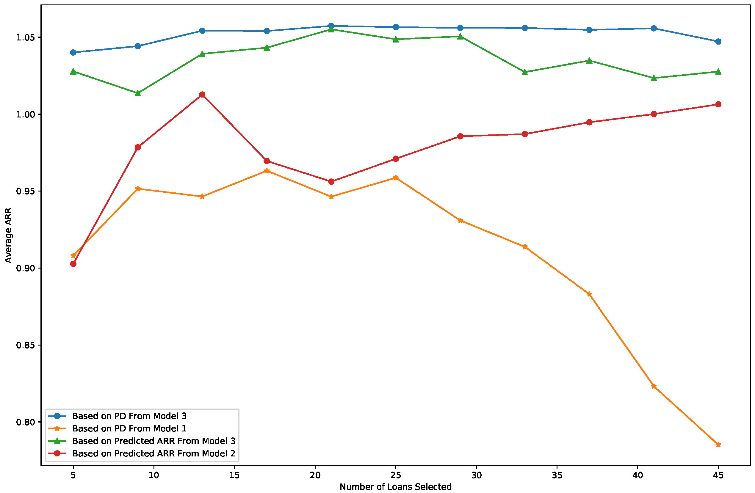
• The average profitability is calculated in terms of the average ARR among the recommended loans. Figure 4 displays the comparison of loan profitability among 4 recommendations. Similar to the logic used in the comparisons of accuracy and RMSE, high-quality loans are those with a low PD in Model 1 or a high predicted ARR in Model 2. For Model 3, two types of recommendations are made based on its two outputs: high-quality loans can be associated with either a low PD or a high predicted ARR. For instance, when the x-axis value in Figure 4 is 45, 45 loans are recommended to investors using different evaluation criteria. Among these 45 loans, the average ARR is approximately 0.78 when selected by Model 1 (orange line) and about 1.01 when selected by Model 2 (red line). For Model 3, the average ARR is 1.05 when selecting loans based on the predicted PD (blue line) and 1.03 when selecting loans based on the predicted ARR (green line). Overall, the average ARR is consistently the highest when loans are selected by Model 3 using the PD output, and it is the second-highest when selected using the predicted ARR output from Model 3.
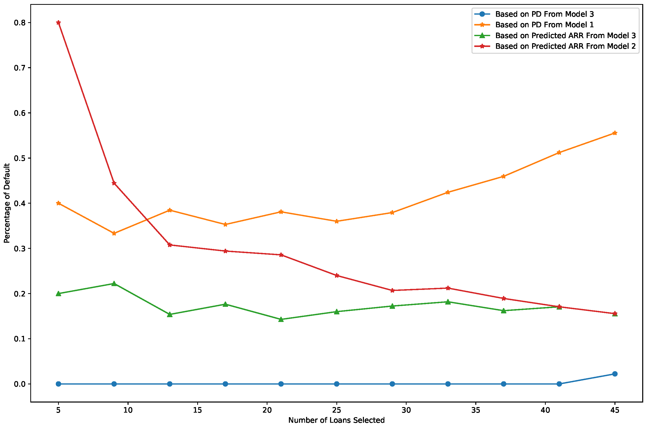
• The default risk is measured as the percentage of defaulted loans among the recommended loans. Figure 5 presents a comparison of risk across the four recommendation methods. The loan selection criteria are the same as those used in the profitability comparison. As shown in Figure 5, the percentage of defaulted loans is very low when loans are selected based on the PD output from Model 3 (blue line), ensuring minimal investment risk. When loans are selected using the predicted ARR from Model 3 (green line), the default rate is the second-lowest among the methods, further demonstrating the model’s ability to balance profitability and risk.
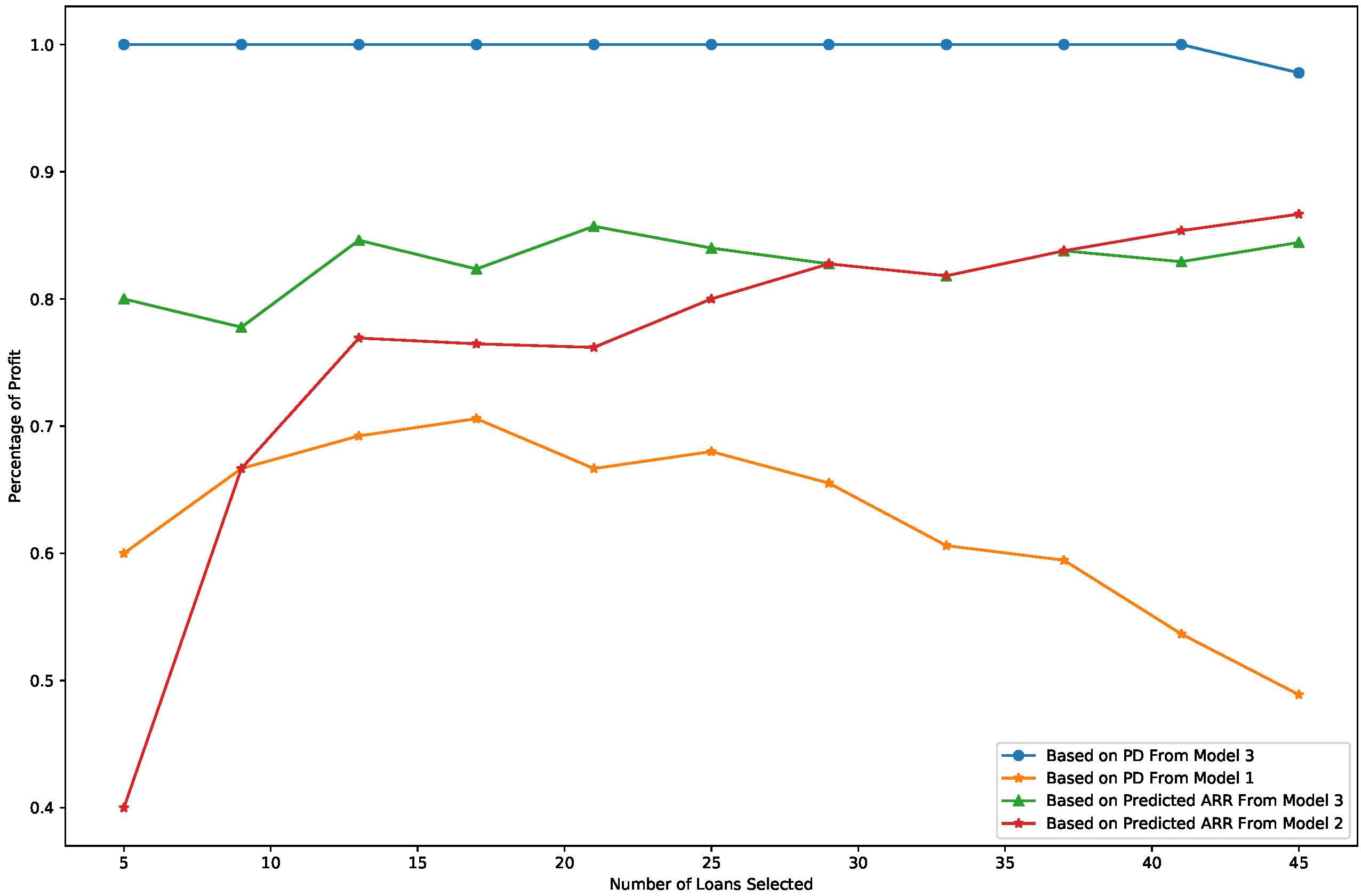
• Portfolio reliability is measured as the percentage of profitable loans among the recommended loans, where profitable loans are defined as those with an ARR greater than 1. Figure 6 illustrates the comparison of portfolio reliability across the models. As shown in Figure 6, the percentage of profitable loans is consistently the highest when loans are selected based on the PD output from Model 3 (blue line), highlighting its superior ability to ensure a reliable portfolio.

To further analyze the differences in loan portfolios recommended by the three models, we examined the composition of the recommended loans when a lender selects 45 loans, categorized by the loan grades provided by the Lending Club platform. The results are presented in

Table 3. Constitution of the top 45 loans selected by Models 1 and 2. Columns “Loan”, “Def”, “Prof”, and $\overline{\mathit{ARR}}$ represent the number of loans, the percentage of defaulted loans, the percentage of profitable loans, and the average ARR within each grade segment, respectively. NA denotes values that cannot be calculated because no loans exist.

	Model 1				Model 2
Grade	Loans	Def	Prof	$\overline{\mathit{ARR}}$	Loans	Def	Prof	$\overline{\mathit{ARR}}$
A	1	0.00	1.00	1.04	23	0.04	0.96	1.05
B	4	0.00	1.00	1.10	10	0.20	0.80	0.91
C	4	0.50	0.50	0.90	9	0.11	1.00	1.10
D	4	0.25	1.00	1.11	2	1.00	0.00	0.60
E	3	0.33	0.67	0.84	1	0.00	1.00	1.15
F	5	0.80	0.20	0.57	NA	NA	NA	NA
G	24	0.75	0.29	0.68	NA	NA	NA	NA
Overall	45	0.58	0.47	0.78	45	0.13	0.89	1.01

and

Table 4. Constitution of the top 45 loans selected by Model 3 using either PD or predicted ARR as the selecting criteria. Columns “Loan”, “Def”, “Prof”, and $\overline{\mathit{ARR}}$ represent the number of loans, the percentage of defaulted loans, the percentage of profitable loans, and the average ARR within each grade segment, respectively. NA denotes values that cannot be calculated because no loans exist.

	Model 3 (Based on PD)				Model 3 (Based on Predicted ARR)
Grade	Loans	Def	Prof	$\overline{\mathit{ARR}}$	Loans	Def	Prof	$\overline{\mathit{ARR}}$
A	30	0.00	1.00	1.04	17	0.12	0.88	1.03
B	10	0.00	1.00	1.08	8	0.13	0.88	1.01
C	5	0.20	0.80	1.00	11	0.18	0.82	1.07
D	NA	NA	NA	NA	2	0.00	1.00	1.17
E	NA	NA	NA	NA	3	0.33	0.67	0.83
F	NA	NA	NA	NA	4	0.25	0.75	1.02
Overall	45	0.02	0.98	1.05	45	0.16	0.84	1.03

.

Table 3 reveals that although Model 1 focuses on minimizing the default risk, it selects five loans with Grade F and 24 loans with Grade G, the grades associated with the highest default rates. This indicates that the traditional credit scoring method may not be effective for investors targeting the top-performing loans. Model 2, on the other hand, primarily selects loans from Grades A and B, successfully capturing one profitable loan from Grade E. However, it also selects two loans from Grade D, both of which default and yield low ARR, highlighting some inconsistencies in its recommendations. However, it selects two loans from Grade D, which are both defaulted and generate a low ARR.

The composition of the top 45 loans selected by Model 3 differs significantly from those chosen by Models 1 and 2. As shown in Table 4, when loans are selected based on the PD output of Model 3, 30 out of the 45 loans are from Grade A, with no loans from Grades D, E, or F. More importantly, only one selected loan defaults, and most are associated with a guaranteed profit. In contrast, when loans are selected based on the predicted ARR from Model 3, 17 of the 45 loans come from Grade A, while the remaining 28 are distributed across Grades B through F. This demonstrates the flexibility and superior reliability of Model 3 in recommending diverse yet profitable loan portfolios.

In summary, the results indicate that the bivariate model improves the prediction of both loan_status and ARR by incorporating their intrinsic interaction, leading to a more effective loan evaluation. Among the outputs, the PD from Model 3 proves to be the most reliable reference for making investment decisions, as it consistently generates loan portfolios with the highest profitability, the lowest risk, and the most reliable portfolios with the highest percentage of profitable loans.

Furthermore, this approach allows investors to diversify their portfolios by increasing the number of loans they invest in without significantly compromising their chances of achieving profitable outcomes.

4. The Proposed Bivariate Method for Correlated and Mixed Outcomes

Before delving into the details of the proposed model, we first introduce the notations used in this article. Following this, we will describe the proposed method and provide the proof of the convexity of the loss function, which ensures the convergence of the learning algorithm. The notations used in the subsequent sections are defined as follows:

• $D={\{d_1,d_2,...,d_N\}}^T$: a data set with N observations, p features, and mixed outcomes;
• i: the observation index, where i = 1, 2, …, N;
• j: the feature index, or the index of independent variables or explanatory variables, where j = 1, 2, …, p;
• $d_i^T$: the data vector for the i-th observation. $d_i^T$ can also be expressed as $\langle \underline{{\mathbf{x}}_{\mathbf{i}}^{\mathbf{T}}},y_{i1},y_{i2}\rangle$, where $\underline{{\mathbf{x}}_{\mathbf{i}}^{\mathbf{T}}}=[1,x_{i1},x_{i2},...,x_{ip}]$ denotes its feature vector with the first element 1 for the interception, $y_{i1}$ is the value of its binary outcome, and $y_{i2}$ is the continuous outcome;
• $p(y_{i1}=k)$: the probability that the ith observation belongs to the kth category, where k is either 1 or 0 for the binary classification problem;
• $\mathit{\beta }$: the coefficient vector estimated by the model, where ${\mathit{\beta }}^T=[{\mathit{\beta }}_0,{\mathit{\beta }}_1,...,{\mathit{\beta }}_p]$;
• $\mathcal{L}$: the loss function;
• $LL$: the log-likelihood function.

4.1. Define the Loss Function

Consider a specific loan i with a discrete binary response, $y_{i1}$, and a continuous response, $y_{i2}$. The discrete outcome $y_{i1}$ is 1 if a certain event occurs for this loan and 0 otherwise. In addition, each observation (i.e., each loan) is associated with a $1\times (p+1)$ feature vector denoted as $\underline{{\mathbf{x}}_{\mathbf{i}}^{\mathbf{T}}}$. We assume the binary outcome $y_{i1}$ follows a Bernoulli distribution, with its density function given by Equation (6). Here, ${\mathit{\beta }}_{\mathbf{1}}$ represents the coefficient vector used to predict $y_{i1}$ through a logistic regression model. The expected value of $y_{i1}$ for the i-th observation is expressed by Equation (7) (Forbes et al. 2011; le Cessie and Van Houwelingen 1994).

$$f\left(y_{i1}\right|{\mathbf{x}}_{\mathbf{i}})=exp\left[y_{i1}\ast {\mathit{\beta }}_{\mathbf{1}}^{\mathbf{T}}\underline{{\mathbf{x}}_{\mathbf{i}}}-log(1+exp\left({\mathit{\beta }}_{\mathbf{1}}^{\mathbf{T}}\underline{{\mathbf{x}}_{\mathbf{i}}}\right))\right]$$

(6)

$$E\left(y_{i1}\right)=prob(y_{i1}=1|\underline{{\mathbf{x}}_{\mathbf{i}}},{\mathit{\beta }}_{\mathbf{1}})={\displaystyle \frac{exp\left({\mathit{\beta }}_{\mathbf{1}}^{\mathbf{T}}\underline{{\mathbf{x}}_{\mathbf{i}}}\right)}{1+exp\left({\mathit{\beta }}_{\mathbf{1}}^{\mathbf{T}}\underline{{\mathbf{x}}_{\mathbf{i}}}\right)}}$$

(7)

Furthermore, we assume that for a given $y_{i1}$, the distribution of $y_{i2}$ is normal or approximately normal. Considering the possible inter-relationship between $y_{i1}$ and $y_{i2}$, we propose that the expectation of $y_{i1}$ serves as a potential predictor for $y_{i2}$. The inter-relationship is mathematically represented in Equation (8), where ${\mathit{\beta }}_{\mathbf{2}}$ is the coefficient vector corresponding to the prediction of $y_{i2}$, and $\gamma$ is a scalar coefficient capturing the inter-relationship between $y_{i1}$ and $y_{i2}$. Therefore, the conditional density function of $y_{i2}$, given the value of $y_{i1}$, can be expressed by Equation (9), where $\sigma$ is the standard deviation of the normal distribution (Fitzmaurice and Laird 1995).

$$E\left(y_{i2}\right)=E\left(y_{i2}\right|\underline{{\mathbf{x}}_{\mathbf{i}}},{\mathit{\beta }}_{\mathbf{2}},E\left(y_{i1}\right))={\mathit{\beta }}_{\mathbf{2}}^{\mathbf{T}}\underline{{\mathbf{x}}_{\mathbf{i}}}+\gamma E\left(y_{i1}\right)$$

(8)

$$f_{y_{i2}|y_{i1}}\left(y_{i2}\right|y_{i1})={\displaystyle \frac{1}{\sqrt{\left(2\pi {\sigma }^2\right)}}}exp\left({\displaystyle \frac{-{[y_{i2}-{\mathit{\beta }}_{\mathbf{2}}^{\mathbf{T}}\underline{{\mathbf{x}}_{\mathbf{i}}}-\gamma E\left(y_{i1}\right)]}^2}{2{\sigma }^2}}\right)$$

(9)

Based on the joint density of ($y_{i1}$, $y_{i2}$) defined in Equation (10), along with the density function for $y_{i1}$ in Equation (6) and the expectation for $y_{i2}$ in Equation (8), the loss for loan i during model training can be formulated as shown in Equation (11). Here, ${\mathcal{L}}_i(y_{i1},y_{i2})$ represents the joint loss, which is the negative log-likelihood function. Additionally, ${\mathcal{L}}_i\left(y_{i1}\right)$ denotes the marginal loss contributed by $y_{i1}$, and ${\mathcal{L}}_i\left(y_{i2}\right|y_{i1})$ represents the conditional loss contributed by $y_{i2}$ given $y_{i1}$ (Atchison and Shen 1980; Cox and Wermuth 1992; Gumbel 1961). Consequently, for the entire training data with N loans, the overall loss function $\mathcal{L}$ is defined in Equation (12), and the model is optimized to minimize $\mathcal{L}$.

$$f_{y_{i1},y_{i2}}(y_{i1},y_{i2})=f_{y_{i1}}\left(y_{i1}\right)f_{y_{i2}|y_{i1}}\left(y_{i2}\right|y_{i1})$$

(10)

$$\begin{array}{cc}\hfill {\mathcal{L}}_i(y_{i1},y_{i2})=& -L{L}_i(y_{i1},y_{i2})\hfill \\ \hfill =& -log\left[f_{y_{i1},y_{i2}}(y_{i1},y_{i2})\right]\hfill \\ \hfill =& -log\left[f_{y_{i1}}\left(y_{i1}\right)\right]-log\left[f_{y_{i2}|y_{i1}}\left(y_{i2}\right|y_{i1})\right]\hfill \\ \hfill =& {\mathcal{L}}_i\left(y_{i1}\right)+{\mathcal{L}}_i\left(y_{i2}\right|y_{i1})\hfill \end{array}$$

(11)

$$\begin{array}{cc}\hfill \mathcal{L}=-LL=& \sum _{i=1}^N{\mathcal{L}}_i(y_{i1},y_{i2})\hfill \\ \hfill =& \sum _{i=1}^N{\mathcal{L}}_i\left(y_{i1}\right)+\sum _{i=1}^N{\mathcal{L}}_i\left(y_{i2}\right|y_{i1})\hfill \\ \hfill =& -\sum _{i=1}^N{y}_{i1}log{\displaystyle \frac{exp\left({\mathit{\beta }}_{\mathbf{1}}^{\mathbf{T}}\underline{{\mathbf{x}}_{\mathbf{i}}}\right)}{1+exp\left({\mathit{\beta }}_{\mathbf{1}}^{\mathbf{T}}\underline{{\mathbf{x}}_{\mathbf{i}}}\right)}}\hfill \\ \hfill & -\sum _{i=1}^N(1-y_{i1})log{\displaystyle \frac{1}{1+exp\left({\mathit{\beta }}_{\mathbf{1}}^{\mathbf{T}}\underline{{\mathbf{x}}_{\mathbf{i}}}\right)}}\hfill \\ \hfill & +\sum _{i=1}^N{\left[y_{i2}-{\mathit{\beta }}_{\mathbf{2}}^{\mathbf{T}}\underline{{\mathbf{x}}_{\mathbf{i}}}-\gamma {\displaystyle \frac{exp\left({\mathit{\beta }}_{\mathbf{1}}^{\mathbf{T}}\underline{{\mathbf{x}}_{\mathbf{i}}}\right)}{1+exp\left({\mathit{\beta }}_{\mathbf{1}}^{\mathbf{T}}\underline{{\mathbf{x}}_{\mathbf{i}}}\right)}}\right]}^2\hfill \end{array}$$

(12)

4.2. Convexity of the Loss Function

In this section, we will mathematically prove that the loss function $\mathcal{L}$, as defined in Equation (12), converges during the training process when an appropriate learning rate is used. Therefore, a reliable optimal solution that minimizes the loss function is guaranteed to be found.

To establish convergence, we first transform the problem into proving the convexity of the loss function, as a convex loss function is guaranteed to converge. According to Definition 1, which outlines the concept of convexity (Roberts 1993), this task can be further reduced to proving the positive semi-definiteness of the Hessian matrix of the given loss function. Lemma 1 highlights an essential property of convex functions (Boyd and Vandenberghe 2004), which will be further referenced during our proof.

Definition 1.

A twice differentiable function $f:{\mathbb{R}}^n\to \mathbb{R}$ is convex if and only if inequality (13) holds:

$$z^T\left[{\displaystyle \frac{{\partial }^{2}f\left(x\right)}{{(\partial x)}^2}}\right]z\ge 0,\forall z$$

(13)

In other words, f is convex if and only if the Hessian matrix ${\displaystyle \frac{{\partial }^{2}f\left(x\right)}{{(\partial x)}^2}}$ is positive semi-definite for all x ∈${\mathbb{R}}^n$.

Lemma 1.

Let f(x), g(x) be two convex functions, then for ${\lambda }_1$, ${\lambda }_2\ge 0$, ${\lambda }_{1}f\left(x\right)+{\lambda }_{2}g\left(x\right)$ is also convex. In other words, non-negative linear combinations of convex functions are also convex.

We now present the proof of the convexity of the loss function.

Proof. 

The loss function $\mathcal{L}$ given in Equation (12) can be expressed as a linear combination of functions (14), (15), and (16). According to Lemma 1, proving the convexity of $\mathcal{L}$ requires demonstrating the convexity of these three functions. Based on Definition 1, this further necessitates proving that the Hessian matrices of functions (14), (15), and (16) are all positive semi-definite.

Without loss of generality, we prove the convexity of function (14), as the convexity of function (15) can be established in a similar manner.

$$\begin{array}{c}\hfill -log{\displaystyle \frac{exp\left({\mathit{\beta }}_{\mathbf{1}}^{\mathbf{T}}\underline{{\mathbf{x}}_{\mathbf{i}}}\right)}{1+exp\left({\mathit{\beta }}_{\mathbf{1}}^{\mathbf{T}}\underline{{\mathbf{x}}_{\mathbf{i}}}\right)}}\end{array}$$

(14)

$$\begin{array}{c}\hfill -log{\displaystyle \frac{1}{1+exp\left({\mathit{\beta }}_{\mathbf{1}}^{\mathbf{T}}\underline{{\mathbf{x}}_{\mathbf{i}}}\right)}}\end{array}$$

(15)

$$\begin{array}{c}\hfill {\left[y_{i2}-{\mathit{\beta }}_{\mathbf{2}}^{\mathbf{T}}\underline{{\mathbf{x}}_{\mathbf{i}}}-\gamma {\displaystyle \frac{exp\left({\mathit{\beta }}_{\mathbf{1}}^{\mathbf{T}}\underline{{\mathbf{x}}_{\mathbf{i}}}\right)}{1+exp\left({\mathit{\beta }}_{\mathbf{1}}^{\mathbf{T}}\underline{{\mathbf{x}}_{\mathbf{i}}}\right)}}\right]}^2\end{array}$$

(16)

The Hessian matrix of function (14) with respect to ${\mathit{\beta }}_{\mathbf{1}}$ is given in Equation (17). Subsequently, Equation (18) is used to determine whether the Hessian matrix is positive semi-definite.

$$\begin{array}{cc}\hfill Hessian\left(f\left({\mathit{\beta }}_{\mathbf{1}}\right)\right)=& \left[{\displaystyle \frac{{\partial }^{2}f\left({\mathit{\beta }}_{\mathbf{1}}\right)}{\partial {\mathit{\beta }}_{\mathbf{1}}\partial {\mathit{\beta }}_{\mathbf{1}}^{\mathbf{T}}}}\right]\hfill \\ \hfill =& {\displaystyle \frac{{\partial }^2}{\partial {\mathit{\beta }}_{\mathbf{1}}\partial {\mathit{\beta }}_{\mathbf{1}}^{\mathbf{T}}}}\left[-log{\displaystyle \frac{exp\left({\mathit{\beta }}_{\mathbf{1}}^{\mathbf{T}}\underline{{\mathbf{x}}_{\mathbf{i}}}\right)}{1+exp\left({\mathit{\beta }}_{\mathbf{1}}^{\mathbf{T}}\underline{{\mathbf{x}}_{\mathbf{i}}}\right)}}\right]\hfill \\ \hfill =& {\displaystyle \frac{1}{1+exp\left({\mathit{\beta }}_{\mathbf{1}}^{\mathbf{T}}\underline{{\mathbf{x}}_{\mathbf{i}}}\right)}}\left(1-{\displaystyle \frac{1}{1+exp\left({\mathit{\beta }}_{\mathbf{1}}^{\mathbf{T}}\underline{{\mathbf{x}}_{\mathbf{i}}}\right)}}\right)\underline{{\mathbf{x}}_{\mathbf{i}}}\underline{{\mathbf{x}}_{\mathbf{i}}^{\mathbf{T}}}\hfill \end{array}$$

(17)

⇒

$$\begin{array}{cc}\hfill & z^T\left[{\displaystyle \frac{{\partial }^{2}f\left({\mathit{\beta }}_{\mathbf{1}}\right)}{\partial {\mathit{\beta }}_{\mathbf{1}}\partial {\mathit{\beta }}_{\mathbf{1}}^{\mathbf{T}}}}\right]z\hfill \\ \hfill =& z^T\left[{\displaystyle \frac{1}{1+exp\left({\mathit{\beta }}_{\mathbf{1}}^{\mathbf{T}}\underline{{\mathbf{x}}_{\mathbf{i}}}\right)}}\left(1-{\displaystyle \frac{1}{1+exp\left({\mathit{\beta }}_{\mathbf{1}}^{\mathbf{T}}\underline{{\mathbf{x}}_{\mathbf{i}}}\right)}}\right)\underline{{\mathbf{x}}_{\mathbf{i}}}\underline{{\mathbf{x}}_{\mathbf{i}}^{\mathbf{T}}}\right]z\hfill \\ \hfill =& {\displaystyle \frac{1}{1+exp\left({\mathit{\beta }}_{\mathbf{1}}^{\mathbf{T}}\underline{{\mathbf{x}}_{\mathbf{i}}}\right)}}\left(1-{\displaystyle \frac{1}{1+exp\left({\mathit{\beta }}_{\mathbf{1}}^{\mathbf{T}}\underline{{\mathbf{x}}_{\mathbf{i}}}\right)}}\right){\left(\underline{{\mathbf{x}}_{\mathbf{i}}^{\mathbf{T}}}z\right)}^2\hfill \end{array}$$

(18)

In Expression (18), we observe that ${\displaystyle \frac{1}{1+exp\left({\mathit{\beta }}_{\mathbf{1}}^{\mathbf{T}}\underline{{\mathbf{x}}_{\mathbf{j}}}\right)}}\in (0,1)$, and consequently, $1-{\displaystyle \frac{1}{1+exp\left({\mathit{\beta }}_{\mathbf{1}}^{\mathbf{T}}\underline{{\mathbf{x}}_{\mathbf{j}}}\right)}}\in (0,1)$ as well. Additionally, it is always true that ${\left(\underline{{\mathbf{x}}_{\mathbf{i}}^{\mathbf{T}}}z\right)}^2\ge 0$ since it is the square of a scalar. Therefore, $z^T\left[{\displaystyle \frac{{\partial }^{2}f\left({\mathit{\beta }}_{\mathbf{1}}\right)}{\partial {\mathit{\beta }}_{\mathbf{1}}\partial {\mathit{\beta }}_{\mathbf{1}}^{\mathbf{T}}}}\right]z$≥ 0 holds for all z. Consequently, ${\displaystyle \frac{{\partial }^{2}f\left({\mathit{\beta }}_{\mathbf{1}}\right)}{\partial {\mathit{\beta }}_{\mathbf{1}}\partial {\mathit{\beta }}_{\mathbf{1}}^{\mathbf{T}}}}$ is positive semi-definite. Based on Definition 1, we conclude that function (14) is convex with respect to ${\mathit{\beta }}_{\mathbf{1}}$.

Similarly, the function provided in Expression (15) is convex with respect to ${\mathit{\beta }}_{\mathbf{1}}$.

With respect to function (16), it can be re-written in matrix form as shown in Expression (19), where ${\mathit{\theta }}^T$ and $\underline{\mathbf{X}}$ are defined in Expression (20) and (21), respectively.

$${(y_{i2}-{\underline{\mathit{\theta }}}^T\underline{\mathbf{X}})}^2$$

(19)

$${\underline{\mathit{\theta }}}^T=\left[{\mathit{\beta }}_{\mathbf{2}}^{\mathbf{T}}\gamma \right]$$

(20)

$$\underline{\mathbf{X}}=\left[\begin{array}{c}\underline{{\mathbf{x}}_{\mathbf{i}}}\\ {\displaystyle \frac{exp\left({\mathit{\beta }}_{\mathbf{1}}^{\mathbf{T}}\underline{{\mathbf{x}}_{\mathbf{i}}}\right)}{1+exp\left({\mathit{\beta }}_{\mathbf{1}}^{\mathbf{T}}\underline{{\mathbf{x}}_{\mathbf{i}}}\right)}}\end{array}\right]$$

(21)

Thus, the first derivative of function (19) with respect to $\mathit{\theta }$ is derived in Equation (22), and its corresponding Hessian matrix is provided in Equation (23).

$$\begin{array}{cc}\hfill & {\displaystyle \frac{\partial }{\partial \mathit{\theta }}}{(y_{i2}-{\underline{\mathit{\theta }}}^T\underline{\mathbf{X}})}^2\hfill \\ \hfill =& 2(y_{i2}-{\underline{\mathit{\theta }}}^T\underline{\mathbf{X}})(-{\underline{\mathbf{X}}}^T)\hfill \\ \hfill =& 2({\underline{\mathit{\theta }}}^T\underline{\mathbf{X}}-y_{i2})\left({\underline{\mathbf{X}}}^T\right)\hfill \end{array}$$

(22)

$$\begin{array}{cc}\hfill Hessian\left(f\right(\mathit{\theta }\left)\right)=& {\displaystyle \frac{{\partial }^{2}f\left(\mathit{\theta }\right)}{\partial \mathit{\theta }\partial {\mathit{\theta }}^{\mathbf{T}}}}\hfill \\ \hfill =& {\displaystyle \frac{{\partial }^2}{\partial \mathit{\theta }\partial {\mathit{\theta }}^{\mathbf{T}}}}\left[{(y_{i2}-{\underline{\mathit{\theta }}}^T\underline{\mathbf{X}})}^2\right]\hfill \\ \hfill =& {\displaystyle \frac{\partial }{\partial {\mathit{\theta }}^{\mathbf{T}}}}\left[2({\underline{\mathit{\theta }}}^T\underline{\mathbf{X}}-y_{i2})\left({\underline{\mathbf{X}}}^T\right)\right]\hfill \\ \hfill =& 2\underline{\mathbf{X}}{\underline{\mathbf{X}}}^T\hfill \end{array}$$

(23)

⇒

$$\begin{array}{cc}\hfill & z^T\left[{\displaystyle \frac{{\partial }^{2}f\left(\mathit{\theta }\right)}{\partial \mathit{\theta }\partial {\mathit{\theta }}^{\mathbf{T}}}}\right]z\hfill \\ \hfill & =z^T\left[2\underline{\mathbf{X}}{\underline{\mathbf{X}}}^T\right]z\hfill \\ \hfill & =2{\left({\underline{\mathbf{X}}}^{T}z\right)}^T{\underline{\mathbf{X}}}^{T}z\hfill \end{array}$$

(24)

It is evident that Equation (24) is always non-negative. Therefore, the function provided in Expression (19) (or equivalently in Expression (16)) is convex. Since $\mathcal{L}$, as defined in Equation (12), is a positive linear combination of functions (14), (15), and (16), we can conclude the convexity of $\mathcal{L}$ based on Lemma 1.    □

4.3. Learning Algorithm of the Bivariate Model

The mini-batch stochastic gradient descent algorithm is employed to learn the parameters in the proposed bivariate model. The partial derivatives with respect to ${\mathit{\beta }}_{\mathbf{1}}$, ${\mathit{\beta }}_{\mathbf{2}}$, and $\gamma$ are derived in Equations (25), (26), and (27), respectively. During each iteration of the training process, the estimations of the coefficient vectors—${\mathit{\beta }}_{\mathbf{1}}$ and ${\mathit{\beta }}_{\mathbf{2}}$, along with the scalar term $\gamma$—are updated until the algorithm converges. The details of the proposed training process for the hybrid bivariate model are outlined in Algorithm 1.

$$\begin{array}{cc}\hfill {\displaystyle \frac{\partial \mathcal{L}}{\partial {\mathit{\beta }}_{\mathbf{1}}}}=& \left({\displaystyle \frac{exp\left({\mathit{\beta }}_{\mathbf{1}}^{\mathbf{T}}\underline{{\mathbf{x}}_{\mathbf{i}}}\right)}{1+exp\left({\mathit{\beta }}_{\mathbf{1}}^{\mathbf{T}}\underline{{\mathbf{x}}_{\mathbf{i}}}\right)}}-y_{i1}\right)\underline{{\mathbf{x}}_{\mathbf{i}}}\hfill \\ \hfill & +2\left(y_{i2}-{\mathit{\beta }}_2^T\underline{{\mathbf{x}}_{\mathbf{i}}}-\gamma {\displaystyle \frac{exp\left({\mathit{\beta }}_{\mathbf{1}}^{\mathbf{T}}\underline{{\mathbf{x}}_{\mathbf{i}}}\right)}{1+exp\left({\mathit{\beta }}_{\mathbf{1}}^{\mathbf{T}}\underline{{\mathbf{x}}_{\mathbf{i}}}\right)}}\right)\left(-\gamma {\displaystyle \frac{exp\left({\mathit{\beta }}_{\mathbf{1}}^{\mathbf{T}}\underline{{\mathbf{x}}_{\mathbf{i}}}\right)}{1+exp\left({\mathit{\beta }}_1^T\underline{{\mathbf{x}}_{\mathbf{i}}}\right)}}\right)\left(1-{\displaystyle \frac{exp\left({\mathit{\beta }}_{\mathbf{1}}^{\mathbf{T}}\underline{{\mathbf{x}}_{\mathbf{i}}}\right)}{1+exp\left({\mathit{\beta }}_{\mathbf{1}}^{\mathbf{T}}\underline{{\mathbf{x}}_{\mathbf{i}}}\right)}}\right)(-\underline{{\mathbf{x}}_{\mathbf{i}}})\hfill \end{array}$$

(25)

$${\displaystyle \frac{\partial \mathcal{L}}{\partial {\mathit{\beta }}_{\mathbf{2}}}}=2\ast \left(y_{i2}-{\mathit{\beta }}_{\mathbf{2}}^{\mathbf{T}}\underline{{\mathbf{x}}_{\mathbf{i}}}-\gamma {\displaystyle \frac{exp\left({\mathit{\beta }}_{\mathbf{1}}^{\mathbf{T}}\underline{{\mathbf{x}}_{\mathbf{i}}}\right)}{1+exp\left({\mathit{\beta }}_{\mathbf{1}}^{\mathbf{T}}\underline{{\mathbf{x}}_{\mathbf{i}}}\right)}}\right)(-\underline{{\mathbf{x}}_{\mathbf{i}}})$$

(26)

$${\displaystyle \frac{\partial \mathcal{L}}{\partial \gamma }}=2\ast \left(y_{i2}-{\mathit{\beta }}_{\mathbf{2}}^{\mathbf{T}}\underline{{\mathbf{x}}_{\mathbf{i}}}-\gamma {\displaystyle \frac{exp\left({\mathit{\beta }}_{\mathbf{1}}^{\mathbf{T}}\underline{{\mathbf{x}}_{\mathbf{i}}}\right)}{1+exp\left({\mathit{\beta }}_{\mathbf{1}}^{\mathbf{T}}\underline{{\mathbf{x}}_{\mathbf{i}}}\right)}}\right)\left(-{\displaystyle \frac{exp\left({\mathit{\beta }}_{\mathbf{1}}^{\mathbf{T}}\underline{{\mathbf{x}}_{\mathbf{i}}}\right)}{1+exp\left({\mathit{\beta }}_{\mathbf{1}}^{\mathbf{T}}\underline{{\mathbf{x}}_{\mathbf{i}}}\right)}}\right)$$

(27)

5. Conclusions and Discussion

Traditionally, credit scoring and profit scoring approaches have been used independently in P2P research for loan evaluation. The single-method loan evaluation approach overlooks the intrinsic correlation between default risk and potential profit. In this article, we propose a bivariate method tailored to the specific needs of the P2P lending market. The primary advantage of this method is its ability to evaluate both risk and profitability for individual loans while accounting for their interdependence, providing a more comprehensive and accurate loan assessment.

Algorithm 1 Learning the bivariate model for the correlated mixed outcomes

1: Input: Data $D={\{d_1,d_2,...,d_N\}}^T$, loss function $\mathcal{L}$, number of epochs S, learning rate $\alpha$, number of mini-batches m. 2: Split D into mini-batches $B_0,...,B_{m-1}$. 3: Initialize ${\beta }_1^0,{\beta }_2^0,{\gamma }^0$. 4: $k\leftarrow 0$ 5: for $s=1$ to S do                                  ▹ Iterate S times 6:   // Start the epoch s 7:   for $j=0$ to $m-1$ do                              ▹ Iterate m times 8:    // Access the j-th mini-batch 9:    ${\mathit{\beta }}_{\mathbf{1}}^{\mathbf{k}+\mathbf{1}}\leftarrow {\mathit{\beta }}_{\mathbf{1}}^{\mathbf{k}}-\alpha {\displaystyle \frac{1}{|B_j|}}{\sum }_{i\in B_j}{\displaystyle \frac{\partial }{\partial {\mathit{\beta }}_{\mathbf{1}}}}\mathcal{L}(d_i=\langle x_i,y_{i1},y_{i2}\rangle )$ 10:    ${\mathit{\beta }}_{\mathbf{2}}^{\mathbf{k}+\mathbf{1}}\leftarrow {\mathit{\beta }}_{\mathbf{2}}^{\mathbf{k}}-\alpha {\displaystyle \frac{1}{|B_j|}}{\sum }_{i\in B_j}{\displaystyle \frac{\partial }{\partial {\mathit{\beta }}_{\mathbf{2}}}}\mathcal{L}(d_i=\langle x_i,y_{i1},y_{i2}\rangle )$ 11:    ${\gamma }^{k+1}\leftarrow {\gamma }^k-\alpha {\displaystyle \frac{1}{|B_j|}}{\sum }_{i\in B_j}{\displaystyle \frac{\partial }{\partial \gamma }}\mathcal{L}(d_i=\langle x_i,y_{i1},y_{i2}\rangle )$ 12:    $k\leftarrow k+1$ 13:   end for 14:   If converges, break 15: end for 16: Output: binary target model ${\mathit{\beta }}_{\mathbf{1}}^{\mathbf{k}}$, continuous target model ${\mathit{\beta }}_{\mathbf{2}}^{\mathbf{k}}$, interaction ${\gamma }^k$.

The effectiveness of the proposed methodology was evaluated using real-world data from the Lending Club, the largest P2P platform in the US. To ensure a comprehensive analysis, we compared the proposed bivariate method with traditional independent loan evaluation approaches, including credit scoring and profit scoring. The results demonstrated that the proposed method consistently outperforms independent approaches by recommending loans with higher profitability and lower risk, offering better investment suggestions for investors. It is worth noting that the evaluation is conducted on a loan portfolio of up to 45 loans. This size is practical for most personal investors, allowing them to diversify their investments across multiple loans while maintaining portfolio quality. For future research, it would be valuable to explore the robustness of the proposed method as the portfolio size increases.

We are also interested in using Data Envelopment Analysis to assess the efficiency of the funds recommended by the model (Lamb and Tee 2012). However, the scalability of DEA as the number of loans and factors increase could present challenges, particularly in handling a larger volume of data and ensuring computational efficiency. Further investigation into how DEA adapts to dynamic and larger-scale datasets will be crucial in improving its practical applicability in real-world P2P lending scenarios.

Furthermore, the dataset is mildly imbalanced, with $80.44\%$ of the loans being non-defaulted and profitable. Concerns may arise regarding the potential bias introduced by this imbalance. In a related study (Wang et al. 2023), a cost-sensitive model was employed to address the imbalance issue. However, we did not observe significant advantages over cost-insensitive methods in selecting profitable loans. Consequently, we did not incorporate a cost-sensitive or weighted-cost technique in this study. Nevertheless, the imbalanced data distribution may introduce some bias in the binary classification process. For researchers applying the model in similar areas, it is advisable to consider cost-sensitive models if the data exhibit a higher degree of imbalance.

Finally, we want to highlight the contribution of this work. To the best of our knowledge, this study is the first to simultaneously evaluate P2P loans based on both risk and profitability while incorporating their intrinsic correlation through a novel loss function. Furthermore, this loss function is not limited to loan evaluation within the P2P domain. It can be generalized to other fields, such as medical research, where predicting correlated outcomes is essential (Gueorguieva and Sanacora 2006; Wassell and Moeschberger 1993). This broader applicability highlights the potential impact and versatility of the proposed methodology.

References

1. Atchison, Jhon, and Sheng M. Shen. 1980. Logistic-normal distributions: Some properties and uses. Biometrika 67: 261–72. [Google Scholar] [CrossRef]
2. Baesens, Bart, Tony Van Gestel, Stijn Viaene, Maria Stepanova, Johan Suykens, and Jan Vanthienen. 1995. Benchmarking state-of-the-art classification algorithms for credit scoring. Journal of the Operational Research Society 54: 627–35. [Google Scholar] [CrossRef]
3. Bastani, Kaveh, Elham Asgari, and Hamed Namavari. 2019. Wide and deep learning for peer-to-peer lending. Expert Systems with Applications 134: 209–24. [Google Scholar] [CrossRef]
4. Boyd, Stephen, and Lieven Vandenberghe. 2004. Convex Optimization. Cambridge: Cambridge University Press. [Google Scholar]
5. Byanjankar, Ajay, and Markus Viljanen. 2019. Predicting expected profit in ongoing peer-to-peer loans with survival analysis-based profit scoring. Paper presented at 11th KES International Conference on Intelligent Decision Technologies (KES-IDT 2019), St. Julians, Malta, June 17–19. [Google Scholar]
6. Byanjankar, Ajay, Markku Heikkilä, and Jozsef Mezei. 2015. Predicting credit risk in peer-to-peer lending: A neural network approach. Paper presented at 2015 IEEE Symposium Series on Computational Intelligence, Cape Town, South Africa, December 7–10. [Google Scholar]
7. Cox, David R., and Nanny Wermuth. 1992. Response models for mixed binary and quantitative variables. Biometrika 79: 441–61. [Google Scholar] [CrossRef]
8. De Leon, Alexander R., and Keumhee Chough Carriere. 2000. On the one-sample location hypothesis for mixed bivariate data. Communications in Statistics-Theory and Methods 29: 2573–81. [Google Scholar] [CrossRef]
9. Emekter, Riza, Yanbin Tu, Benjamas Jirasakuldech, and Min Lu. 2015. Evaluating credit risk and loan performance in online Peer-to-Peer (P2P) lending. Applied Economics 47: 54–70. [Google Scholar] [CrossRef]
10. Everett, Craig R. 2019. Origins and development of credit-based crowdfunding. Banking and Finance Review 11: 1–32. [Google Scholar] [CrossRef]
11. Fitzmaurice, Garrett M., and Nan M. Laird. 1995. Regression models for a bivariate discrete and continuous outcome with clustering. Journal of the American statistical Association 90: 845–52. [Google Scholar] [CrossRef]
12. Forbes, Catherine, Merran Evans, Nicholas Hastings, and Brian Peacock. 2011. Statistical Distributions. Hoboken: John Wiley & Sons. [Google Scholar]
13. Gueorguieva, Ralitza V., and Gerard Sanacora. 2006. Joint analysis of repeatedly observed continuous and ordinal measures of disease severity. Statistics in Medicine 25: 1307–22. [Google Scholar] [CrossRef]
14. Gumbel, Emil J. 1961. Bivariate logistic distributions. Journal of the American Statistical Association 56: 335–49. [Google Scholar] [CrossRef]
15. Guo, Yanhong, Wenjun Zhou, Chunyu Luo, Chuanren Liu, and Hui Xiong. 2016. Instance-based credit risk assessment for investment decisions in P2P lending. European Journal of Operational Research 249: 417–26. [Google Scholar] [CrossRef]
16. Hand, David J. 2009. Measuring classifier performance: A coherent alternative to the area under the ROC curve. Machine Learning 77: 103–23. [Google Scholar] [CrossRef]
17. Kim, Ji-Yoon, and Sung-Bae Cho. 2019. Predicting repayment of borrows in peer-to-peer social lending with deep dense convolutional network. Expert Systems 54: e12403. [Google Scholar] [CrossRef]
18. Lamb, John, and Kaihong Tee. 2012. Data Envelopment Analysis Models of Investment Funds. European Journal of Operational Research 216: 687–96. [Google Scholar] [CrossRef]
19. le Cessie, Saskia, and Johannes C. Van Houwelingen. 1994. Logistic regression for correlated binary data. Journal of the Royal Statistical Society: Series C Applied Statistics 43: 95–108. [Google Scholar] [CrossRef]
20. Ma, Xiaojun, Jinglan Sha, Dehua Wang, Yuanbo Yu, Qian Yang, and Xueqi Niu. 2018. Study on a prediction of P2P network loan default based on the machine learning LightGBM and XGboost algorithms according to different high dimensional data cleaning. Electronic Commerce Research and Applications 31: 24–39. [Google Scholar] [CrossRef]
21. Malekipirbazari, Milad, and Vural Aksakalli. 2015. Risk assessment in social lending via random forests. Expert Systems with Applications 42: 4621–31. [Google Scholar] [CrossRef]
22. Pierrakis, Yannis. 2018. Banking on Each Other: Peer-to-peer lending to business: Evidence from funding circle. In Electronic Commerce Research and Applications. London: Nesta. [Google Scholar]
23. Roberts, Arthur Wayne. 1993. Convex functions. In Handbook of Convex Geometry. Amsterdam: Elsevier, vol. 10, pp. 1081–104. [Google Scholar]
24. Serrano-Cinca, Carlos, and Begoña Gutiérrez-Nieto. 2016. The use of profit scoring as an alternative to credit scoring systems in peer-to-peer (P2P) lending. Decision Support Systems 89: 113–22. [Google Scholar] [CrossRef]
25. Tang, Huan. 2019. Peer-to-peer lenders versus banks: Substitutes or complements? The Review of Financial Studies 32: 1900–38. [Google Scholar] [CrossRef]
26. Thmasebinejad, Z., and E. Tabrizi. 2015. Sensitivity analysis in correlated bivariate continuous and binary responses. Applications and Applied Mathematics: An International Journal (AAM) 10: 37. [Google Scholar]
27. Tsoumakas, Grigorios, Eleftherios Spyromitros-Xioufis, Aikaterini Vrekou, and Ioannis Vlahavas. 2014. Multi-target regression via random linear target combinations. Paper presented at Joint European Conference on Machine Learning and Knowledge Discovery in Databases, Nancy, France, September 14–18; pp. 225–40. [Google Scholar]
28. Wang, Yan, and Xuelei Sherry Ni. 2020a. Improving Investment Suggestions for Peer-to-Peer Lending via Integrating Credit Scoring into Profit Scoring. Paper presented at 2020 ACM Southeast Conference (ACMSE 2020), Tampa, FL, USA, April 2–4. [Google Scholar]
29. Wang, Yan, and Xuelei Sherry Ni. 2020b. Risk Prediction of Peer-to-Peer Lending Market by a LSTM Model with Macroeconomic Factor. Paper presented at 2020 ACM Southeast Conference (ACMSE 2020), Tampa, FL, USA, April 2–4. [Google Scholar]
30. Wang, Yan, Xuelei Sherry Ni, and Xiao Huang. 2023. Towards Profitability: A Profit-Sensitive Multinomial Logistic Regression for Credit Scoring in Peer-to-Peer Lending. Paper presented at Future Technologies Conference (FTC) 2022, Vancouver, BC, Canada, October 19–20; Cham: Springer International Publishing, vol. 1, pp. 696–718. [Google Scholar]
31. Wassell, James T., and Melvin L. Moeschberger. 1993. A bivariate survival model with modified gamma frailty for assessing the impact of interventions. Statistics in Medicine 12: 241–48. [Google Scholar] [CrossRef] [PubMed]
32. Xia, Yufei, Chuanzhe Liu, and Nana Liu. 2017a. Cost-sensitive boosted tree for loan evaluation in peer-to-peer lending. Electronic Commerce Research and Applications 24: 30–49. [Google Scholar] [CrossRef]
33. Xia, Yufei, Chuanzhe Liu, YuYing Li, and Nana Liu. 2017b. A boosted decision tree approach using Bayesian hyper-parameter optimization for credit scoring. Expert Systems with Applications 78: 225–41. [Google Scholar] [CrossRef]
34. Ye, Xin, Lu-an Dong, and Da Ma. 2018. Loan evaluation in P2P lending based on random forest optimized by genetic algorithm with profit score. Electronic Commerce Research and Applications 32: 23–36. [Google Scholar] [CrossRef]
Figure 1. ARR across different grades in the Lending Club data.
Risks 13 00033 g001
Figure 2. Accuracy rate of the selected loans.
Risks 13 00033 g002
Figure 3. RMSE of the selected loans.
Risks 13 00033 g003
Figure 4. Average ARR of the selected loans.
Risks 13 00033 g004
Figure 5. Percentage of default loans.
Risks 13 00033 g005
Figure 6. Percentage of profitable loans.
Risks 13 00033 g006